CONNECTMTY
Graph Traversal Algorithms
Depth-first search is a member of a family of graph traversal algorithms that
are quite natural when viewed nonrecursively. Any one of these methods can
be used to solve the simple connectivity problems posed in the last chapter.
In this section, we’ll see how one program can be used to implement graph
traversal methods with quite different characteristics, merely by changing the
value of one variable. This method will be used to solve several graph problems
in the chapters which follow.
Consider the analogy of traveling through a maze. Any time we face a
choice of several vertices to visit, we can only go along a path one of them,
so we must “save” the others to visit later. One way to implement a program
based on this idea is to remove the recursion from the recursive depth-first
algorithm given in the previous chapter. This would result in a program that
saves, on a stack, the point in the adjacency list of the vertex being visited
at which the search should resume after all vertices connected to previous
vertices on the adjacency list have been visited. Instead of examining this
implementation in more detail, we’ll look at a more general framework which
encompasses several algorithms.
We begin by thinking of the vertices as being divided into three classes:
tree (or visited) vertices, those connected together by paths that we’ve trav-
ersed; fringe vertices, those adjacent to tree vertices but not yet visited; and
unseen vertices, those that haven’t been encountered at all yet. To search a
connected component of a graph systematically (implement the visit procedure
of the previous chapter), we begin with one vertex on the fringe, all others
unseen, and perform the following step until all vertices have been visited:
“move one vertex (call it from the fringe to the tree, and put any unseen
vertices adjacent to x on the fringe.”
Graph traversal methods differ in how
it is decided which vertex should be moved from the fringe to the tree.
For depth-first search, we always want to choose the vertex from the

fringe that was most recently encountered. This can be implemented by
always moving the first vertex on the fringe to the tree, then putting the
unseen vertices adjacent to that vertex (x) at the front of the fringe and
moving vertices adjacent to which happen to be already on the fringe to the
front. (Note carefully that a completely different traversal method results if
we leave untouched the vertices adjacent to x which are already on the fringe.)
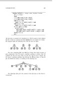
For example, consider the undirected graph given at the beginning of
this chapter. The following table shows the contents of the fringe each time
a vertex is moved to the tree; the corresponding search tree is shown at the
right:
CHAPTER 30
394
A
G
E
D
F
C
H
I
J
M
L
K
B
A
G B C F
ECHJLBF
DFCHJLB
FCHJLB

CHJLB
H J L B
I JLB
J L B
MLKB
LKB
K B
B
In this algorithm, the fringe essentially operates as a pushdown stack: we
remove a vertex (call it from the beginning of the fringe, then go through
x’s edge list, adding unseen vertices to the beginning of the fringe, and moving
fringe vertices to the beginning. Note that this is not strictly a stack, since
we use the additional operation of moving a vertex to the beginning. The
algorithm can be efficiently implemented by maintaining the fringe as a linked
list and keeping pointers into this list in an array indexed by vertex number:
we’ll omit this implementation in favor of a program that can implement other
traversal strategies as well.
This gives a different depth-first search tree than the one drawn in the
biconnectivity section above because x’s edges are put on the stack one at a
time, so their order is reversed when the stack is popped. The same tree as
for recursive depth-first search would result if we were to append all of z’s
edge list on the front of the stack, then go through and delete from the stack
any other occurrences of vertices from x’s edge list. The reader might find it
interesting to compare this process with the result of directly removing the
recursion from the visit procedure of the previous chapter.
By itself, the fringe table does not give enough information to reconstruct
the search tree. In order to actually build the tree, it is necessary to store,
with each node in the fringe table, the name of its father in the tree. This
is available when the node is entered into the table (it’s the node that caused
the entry), it is changed whenever the node moves to the front of the fringe,

and it is needed when the node is removed from the table (to determine where
in the tree to attach it).
A second classic traversal method derives from maintaining the fringe
as a queue: always pick the least recently encountered vertex. This can be
maintained by putting the unseen vertices adjacent to x at the end of the fringe
395
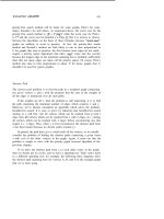
in the general strategy above. This method is called breadth-first search: first
we visit a node, then all the nodes adjacent to it, then all the nodes adjacent
to those nodes, etc. This leads to the following fringe table and search tree
for our example graph:
A
F
C
B
G
E
D
L
J
H
M
K
I
A
F C B G
C B G E
B G E D
G E D
E D L J
D L J H

L J H
JHM
HMK
MKI
K I
I
D
H
We remove a vertex (call it from the beginning of the fringe, then go
through edge list, putting unseen vertices at the end of the fringe. Again,
an efficient implementation is available using a linked list representation for
the fringe, but we’ll omit this in favor of a more general method.
A fundamental feature of this general graph traversal strategy is that the
fringe is actually operating as a priority queue: the vertices can be assigned
priorities with the property that the “highest priority” vertex is the one moved
from the fringe to the tree. That is, we can directly use the priority queue
routines from Chapter 11 to implement a general graph searching program.
For the applications in the next chapter, it is convenient to assign the highest
priority to the lowest value, so we assume that the inequalities are switched
in the programs from Chapter 11. The following program is a “priority first
search” routine for a graph represented with adjacency lists (so it is most
appropriate for sparse graphs).
396
CHAPTER 30
procedure sparsepfs;
var now, k: integer;
link;
begin
for to V do
begin end;

pqconstruct;
repeat
if then
begin end
t:=adj[k];
while do
begin
if then
if and then
begin priority); :=k end;
end
until pqempty;
end;
(The functions onpq and pqempty are priority queue utility routines which
are easily implemented additions to the set of programs given in Chapter 11:
pqempty returns true if the priority queue is empty; onpq returns true if the
given vertex is currently on the priority queue.) Below and in Chapter 31, we’ll
see how the substitution of various expressions for priority in this program
yields several classical graph traversal algorithms. Specifically, the program
operates as follows: first, we give all the vertices the sentinel value unseen
(which could be and initialize the dad array, which is used to store
the search tree. Next we construct an indirect priority queue containing all
the vertices (this construction is trivial because the values are initially all the
same). In the terminology above, tree vertices are those which are not on
the priority queue, unseen vertices are those on the priority queue with value
unseen, and fringe vertices are the others on the priority queue. With these
conventions understood, the operation of the program is straightforward: it
repeatedly removes the highest priority vertex from the queue and puts it on
the tree, then updates the priorities of all fringe or unseen vertices connected
to that vertex.

If all vertices on the priority queue are unseen, then no vertex previously
397
encountered is connected to any vertex on the queue: that is, we’re entering
a new connected component. This is automatically handled by the priority
queue mechanism, so there is no need for a separate visit procedure inside a
main procedure. But note that maintaining the proper value of now is more
complicated than for the recursive depth-first search program of the previous
chapter. The convention of this program is to leave the val entry unseen and
zero for the root of the depth-first search tree for each connected component:
it might be more convenient to set it to zero or some other value (for example,
now) for various applications.
Now, recall that now increases from 1 to V during the execution of the
algorithm so it can be used to assign unique priorities to the vertices. If we
change the two occurrences of priority in sparsepfs to V-now, we get
first search, because newly encountered nodes have the highest priority. If
we use now for priority we get breadth-first search, because old nodes have
the highest priority. These priority assignments make the priority queues
operate like stacks and queues as described above. (Of course, if we were only
interested in using depth-first or breadth-first search, we would use a direct
implementation for stacks or queues, not priority queues as in sparsepfs.)
In the next chapter, we’ll see that other priority assignments lead to other
classical graph algorithms.
The running time for graph traversal when implemented in this way
depends on the method of implementing the priority queue. In general, we
have to do a priority queue operation for each edge and for each vertex, so the
worst case running time should be proportional to (E + V) log V if the priority
queue is implemented as a heap as indicated. However, we’ve already noted
that for both depth-first and breadth-first search we can take advantage of
the fact that each new priority is the highest or the lowest so far encountered
to get a running time proportional to E + V. Also, other priority queue

implementations might sometimes be appropriate: for example if the graph is
dense then we might as well simply keep the priority queue as an unordered
array. This gives a worst case running time proportional to E + (or just
since each edge simply requires setting or resetting a priority, but each
vertex now requires searching through the whole queue to find the highest
priority vertex. An implementation which works in this way is given in the
next chapter.
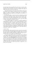
The difference between depth-first and breadth-first search is quite evi-
dent when a large graph is considered. The diagram at left below shows the
edges and nodes visited when depth-first search is halfway through the maze
graph of the previous chapter starting at the upper left corner; the diagram
at right is the corresponding picture for breadth-first search: