MÔ HÌNH HOÁ CỦA TỪ TRƯỜNG VÀ DÒNG ĐIỆN XOÁY TRONG MÀN CHẮN ĐIỆN TỪ BẰNG PHƯƠNG PHÁP LIÊN KẾT BÀI TOÁN NHỎ

Bạn đang xem bản rút gọn của tài liệu. Xem và tải ngay bản đầy đủ của tài liệu tại đây (656.82 KB, 6 trang )

(1)<div class='page_container' data-page=1>

; Email: 7

MODELING OF MAGNETIC FIELDS AND EDDY CURRENT LOSSES IN

ELECTROMAGNETIC SCREENS BY A SUBPROBLEM METHOD

Dang Quoc Vuong*

School of Electrical Engineering, Hanoi University of Science and Technology

ABSTRACT

The aim of this paper is based on a subproblem technique with the magnetic vector potential
formulation to compute magnetic fields, eddy currents and Joule power losses in electromagnetic
screens that are extreamly difficult to perform by a finite element method. The subproblem method
is herein developed for coupling problems in two steps: A problem starting from simplified models
with stranded inductors and thin screen models can be also first considered. Then a correction
problem with the actual volume thin regions is added to correct inaccuracies from previous
problem. All the steps are separately performed with different meshes and geometries, which
facilitates meshing and speeding up the calculation of each problem.

Keywords: Magnetic field, Eddy current, Joule power loss, Electromagnetic screen,

Magnetodynamics, Subproblem method (SPM), Magnetic vector potential.

Received: 18/10/2018; Revised: 16/11/2018; Approved: 28/12/2018

MƠ HÌNH HỐ CỦA TỪ TRƯỜNG VÀ DỊNG ĐIỆN XỐY TRONG MÀN

CHẮN ĐIỆN TỪ BẰNG PHƯƠNG PHÁP LIÊN KẾT BÀI TOÁN NHỎ

Đặng Quốc Vương*

Viện Điện - Trường Đại học Bách khoa Hà Nội

TĨM TẮT

Mục đích của bài bài báo được dựa trên phương pháp bài toán nhỏ với cơng thức véc tơ từ thế để
tính tốn từ trường, dịng điện xốy và tổn hao cơng suất trong các màn chắn điện từ, mà khó có
thể thực hiện trực tiếp bằng phương pháp phần tử hữu hạn. Ở đây, phương pháp bài toán nhỏ được
phát triển để liên kết các bài toán theo hai bước: Một bài tốn với mơ hình đơn giản (các cuộn dây
và màn chắn điện từ) được giải trước, sau đó một bài toán hiệu chỉnh được thêm vào để hiệu chỉnh
sai số do bài toán trước gây ra. Tất cả các bước đều được thực hiện độc lập với các lưới và miền
hình học khác nhau, điều này tạo thuận lợi cho việc chia lưới cũng như tăng tốc độ tính tốn của
mỗi một bài tốn.

Keywords: Từ trường, dịng điện xốy, tổn hao cơng suất, màn chắn điện từ, bài toán từ động,

phương pháp bài toán nhỏ (SPM), véc tơ từ thế.

Ngày nhận bài: 18/10/2018; Ngày hoàn thiện: 16/11/2018;Ngày duyệt đăng: 28/12/2018

</div>
(2)<div class='page_container' data-page=2>

; Email: 
INTRODUCTION

Many papers have been applied a subproblem
method (SPM) for computing electromagnetic
fields (eddy current, magnetic flux density
and magnetic filed) and correcting
inaccuracies of fields in the vicinity of thin
shell models in three steps [1-5]. In this paper,
the SPM is extended for coupling subprolems
(SPs) in two steps: A problem starting from

simplified models with stranded inductors
(Fig. 1, top right) and thin screen models can 
be also first considered, followed by a
correction problem (Fig. 1, bottom) with the 
actual volume thin regions.

The key point of this method allows to benefit
from previous computations instead of
starting a new complete finite element (FE)
solution of thin shell model for any variation
of geometrical or physical characteristics.
Thus, each SP is solved on its own domain
and mesh (Fig. 2), which facilitates meshing
and may increase computational efficiency in
each step.

The method is is validated on a test practical
problem. Its main advantages are pointed out.

Figure 1. Decomposition of a complete problem

into two subproblems

Figure 2. Decomposition of a complete mehs into

two sub-meshes: stranded inductor and thin shell 
mesh (top), actual volume mesh (bottom).

DEFINTION OF THE SUBPROBLEM

METHOD

Canonical Magnetodynamic problem 
A canonical magnetodynamic problem i, to be 
solved at step i of the SPM, is defined in a Ω𝑖,
with boundary 𝑖= Γℎ,𝑖∪ Γ𝑏,𝑖. Subscript i

refers to the associated problem i. The 
equations, material relations, boundary
conditions (BCs) and interface conditions
(ICs) of SPs are [5-11]

curl 𝒉𝑖 = 𝒋𝑖, div 𝒃𝑖= 0, curl 𝒆𝑖 = −𝝏𝑡𝒃𝑖
(1a-b-c)
𝒉𝑖 = 𝜇𝑖−1𝒃

𝑖+ 𝒉𝑠,𝑖, 𝒋𝑝= 𝜎𝑝𝒆𝑝+ 𝒋𝑠,𝑝 (2a-b)

𝒏 × 𝒉𝑖 = 𝒋𝑓,𝒊, 𝒏 × 𝒃𝑖|Γ𝑏,𝑖= 𝒇𝑓,𝑖 (3a-b)

where 𝒉𝑖 is the magnetic field, 𝒃𝑖 is the
magnetic flux density, 𝒆𝑖 is the electric field,
𝒋𝑖 current density, 𝜇𝑖 is the magnetic

permeability and 𝜎𝑖 is the electric

conductivity and n is the unit normal exterior 
to Ω𝑝

The fields 𝒃𝑠,𝑖 and 𝒋𝑠,𝑝 in (2a-b) are volume

sources (VSs). With the SPM, 𝒉𝑠,𝑖 is also

used for expressing changes of permeability
and 𝒋𝑠,𝑖 for changes of conductivity. For

changes in a region, from 𝜇𝑝 and 𝜎𝑝 for
problem (i =p) to 𝜇𝑘 and 𝜎𝑘 for problem (i =

k), the associated VSs 𝒃𝑠,𝑖 and 𝒋𝑠,𝑖 are [2-5].

𝒉𝑠,𝑘= (𝜇𝑘−1− 𝜇𝑝−1)𝒃𝑝, (4)

𝒋𝑠,𝑘= (𝜎𝑘− 𝜎𝑝)𝒆𝑝 (5)

for the total fields to be related by 𝒉𝑝+ 𝒉𝑘 =
(𝜇𝑘−1(𝒃𝑝+ 𝒃𝑘) and 𝒋𝑝+ 𝒋𝑘 = 𝜎𝑘(𝒆𝑝+ 𝒆𝑘).

Γ = Γh∪Γe

Γk=Γh ,k∪Γe,k

Ωc,k

ΩC

c,k

n
n

n t ransit ion layer

act ual volume
air

t hin region(Ωt) Γt

ΩC

c

Ωsor Ωm

js, hs

Ωsor Ωm

γt=γf

...+

t hin shell

</div>
(3)<div class='page_container' data-page=3>

; Email: 9
The surface fields 𝒋𝑓,𝑖 and 𝒇𝑓,𝑖 in (3a-b) are

defined possible SSs that account for
particular phenomena occurring in the thin
region between γ𝑖+ and γ

𝑖

− [2-7]. This is the

case when some field traces in a SP 𝑝( 𝑖 = 𝑝)

are forced to be discontinuous. The continuity
has to be recovered after a correction via a
SP 𝑘 (𝑖 = 𝑘). The SSs in SP 𝑘 are thus to be
fixed as the opposite of the trace solution of
SP 𝑝 [2-5].

Constraints between thin shell and 
correction

The thin shell (TS) model [2-4] written with
the 𝒃𝑖-formulation, requires a free (unknown)
discontinuity 𝒂𝑑,𝑡,𝑖 of the tangential

component 𝒂𝑡,𝑖 = (𝒏 × 𝒂𝑖) × 𝒏 of 𝒂𝑖 through

the TS, i.e.
[𝒏 × 𝒂𝑡,𝑖]Γ

𝑡,𝑖 = 𝒏 × 𝒂𝑑,𝑡,𝑖 (6)

with a fixed zero value along the TS border
∂Γ𝑡,𝑖, which neglects the magnetic flux
entering there. To explicitly express this
discontinuity, one defines [2-5]

𝒂𝑖|Γ𝑡,𝑖 = 𝒂𝑐,𝑖+ 𝒂𝑑,𝑖, (7)

where 𝒂𝑐,𝑖 is the continuous component of 𝒂𝑖.
In addition, the constraint for SPs are 
respectively expressed via SSs and VSs. SSs
in (3a-b) are defined via the BCs and ICs of

impedance-type BC combined with

contributions from SP 𝑖 (𝑖 = 𝑝, 𝑘) [2-5]. One
has [4],

[𝒏 × 𝒉] = [𝒏 × 𝒉𝑝]Γ

𝑡,𝑘+ [𝒏 × 𝒉𝑘]Γ𝑡,𝑘 =

−𝜎𝛽𝜕𝑡(2𝒂𝑐,𝑖+𝒂𝑑,𝑖),

(8)𝛽 = 𝛾𝑖−1tanh (𝑑𝑖𝛾𝑖

2 ) , 𝛾𝑖 =
1+𝑗

𝛿𝑖 ,

𝛿𝑖 = √

2
𝜔𝜇𝜎

where di is the local TS) thickness 𝛾𝑖, 𝛿𝑖 is the
skin depth in the TS, 𝜔 = 2𝜋𝑓 with f is the
frequency, j is the imaginary unit. The VSs 
can be defined in (4) and (5).

Finite element weak formulation

Equations (1b-c) are fulfilled via the
definition of a magnetic vector potential 𝒂𝑖

and an electric scalar potential 𝜈𝑖, leading to

the 𝒂𝑖- formulation, with

curl 𝒂𝑖= 𝒃𝑖, 𝒆𝑖 = −𝝏𝑡𝒂𝑖− grad 𝜈𝑖, (9a-b)

𝒏 × 𝒂𝑖|Γ𝑏,𝑖 = 𝒂𝑓,𝑖. (10)

The weak 𝒃𝑖-formulation (in terms of 𝒂𝑖) of

SP 𝑖 (i



p, k) is obtained from the weak form

of the Ampère equation (1a), i.e. [5] - [11]
(𝜇𝑖−1curl 𝒂𝑖, curl 𝒂𝑖′)

Ω𝑖+ (𝒉𝑠,𝑖, curl 𝒂𝑖

′)

Ω𝑖

+(𝜎𝑖𝜕𝑖𝒂𝑖, 𝒂𝑖′)

Ω𝑐,𝑖+ (𝜎𝑖grad 𝜈𝑖, 𝒂𝑖

′)

Ω𝑐,𝑖

+< 𝒏 × 𝒉𝑖, 𝒂𝑖′ >

Γℎ,𝑖−Γ𝑡,𝑖

+ < [𝒏 × 𝒉𝑖]Γ𝑡,𝑖, 𝒂𝑖′ >Γ𝑡,𝑖
= (𝒋𝑖, 𝒂𝑖′)

Ω𝑠,𝑖, ∀ 𝒂𝑖
′ ∈ 𝐹

𝑖1(Ω𝑖) (11)

𝑐,𝑖, gauged in 𝑐,𝑖𝐶 , and containing the basis

functions for 𝒂𝑖 as well as for the test

function 𝒂𝑖′ (at the discrete level, this space is

defined by edge FEs; the gauge is based on
the tree-co-tree technique); (·, ·) and
< ·, · > respectively denote a volume integral
in  and a surface integral on  of the
product of their vector field arguments. The
surface integral term on Γℎ,𝑖-Γ𝑡,𝑖 accounts for

natural BCs of type (3a), usually zero.

The term < [𝒏 × 𝒉𝑖]Γ𝑡,𝑖, 𝒂𝑖′ > in (11) is
defined via (8), that is

< [𝒏 × 𝒉𝑖]Γ𝑡,𝑖, 𝒂𝑖′ > =

< −𝜎𝛽𝜕𝑡(2𝒂𝑐,𝑖+ 𝒂𝑑,𝑖, 𝒂𝑖′ >, (12)

Once obtained, the TS solution is then
corrected by a correction problem that
overcomes the TS assumption [2-5].

At the discrete level, the source 𝒂𝑝(𝑖 = 𝑝),

initially in mesh of SP𝑢 has to be projected in

</div>
(4)<div class='page_container' data-page=4>

; Email: 
sources is crucial for the efficiency of the

method.

Projections of Solutions between Meshes 
Some parts of a previous solution 𝒂𝑝 serve as
sources in a subdomain 𝑝𝑘 of the

current problem SP𝑘. At the discrete level,

this means that this source quantity 𝒂𝑝 has to
be expressed in the mesh of problem SP𝑘,

while initially given in the mesh of problem
SP𝑝. This can be done via a projection method

[2-4] of its curl limited to 𝑘, i.e.

(curl 𝒂𝑝, curl 𝒂𝑘′)Ω

𝑘= (curl 𝒂𝑘, curl 𝒂𝑘

′)

Ω𝑘,

∀ 𝒂𝑘′ ∈ 𝐹𝑘1(Ω𝑘) (10)

where 𝐹𝑘1(Ω𝑘) is a gauged curl-conform

function space for the k-projected source 𝒂𝑝

(the projection of 𝒂𝑝 on mesh SP𝑘) and the
test function 𝒂𝑘′.

APPLICATION TEST

The test problem is based on TEAM problem
21 (2D-model, page 4) [12], with two
inductors and a magnetic plate/screen (Fig. 3),
with f = 50Hz, 𝜇𝑟 = 200, 𝜎 = 6.484MSm.

Figure 3. Geometry of TEAM problem 21.

The problem is considered in two steps: the
distribution of magnetic flux density
generated by imposed electric currents
flowing in stranded inductors is pointed out in
Figure 4 (top). Then volume correction SP𝑘

replaces the TS plate with classical volume
FEs covering the plates and their
neighborhood, with an adequate refined mesh,

that does not include inductors and TS plate
anymore (Fig. 4, bottom), to correct errors 
arising from the TS plate [2-4]. The
distribution of eddy current density along the
volume correction is shown in Figure 5.

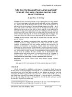
The computed results of magnetic flux
density and Joule power loss in the plate
checked to be close to the measured results
for different parameters of exciting currents
(proposed by author in [12]) are shown in
Figure 6 and Figure 7. The everage errors
between computed and measured methods on
the magnetic flux density are lower than 7%,
and are lower 10% for Joule power losses. It
can be shown that there is a very good
agreement between two methods.

This test problem has been successfully
applied to standardize the type and material of
the plate in practice.

Figure 4. Magnetic flux density for stranded

inductors and TS plate SP𝑝 (top), the correction

SP𝑘 with an actual screen (bottom) (𝜇𝑟=

</div>
(5)<div class='page_container' data-page=5>

; Email: 11

Figure 5. Eddy current along the plate/screen for 
 the correction SP𝑘 with an actual creen (𝜇𝑟=

200, 𝜎 = 6.484MSm, 𝑓 = 50Hz, 𝑑 = 10mm).

Figure 6. Comparison of the computed and

measured Joule power loss in the plate (𝜇𝑟=

100, 𝜎 = 6.484MSm, 𝑓 = 50Hz, 𝑑 = 5mm).

Figure 7. Comparison of the computed and

measured magnetic flux density in the plate 
(𝜇𝑟= 100, 𝜎 = 6.484MSm , 𝑓 = 50Hz, 𝑑 = 5mm).

CONCLUSIONS

All the steps of the subproblem technique
have been presented by coupling SPs in two
steps. The accuracies of magnetic flux density
and Joule power losses are successfully
obtained in the plate/screen. In particular,
they have been checked to be close with the
measured results [12]. Moreover, The

correction is also directly linked to the
volumic mesh of the plate/screen and its
eneighboring, that permit to reduce the
meshing efforts. The method allows to use
previous local meshes instead of starting a
new complete mesh for any postion of the
plate/screen.

REFERENCES

1. Vuong Q. Dang, P. Dular R.V. Sabariego, L.
Krähenbühl, C. Geuzaine, “Subproblem Approach 
for Modelding Multiply Connected Thin Regions 
with an h-Conformal Magnetodynamic Finite 
Element Formulation”, in EPJ AP., vol. 63, 
no.1, 2013.

2. Vuong Q. Dang, P. Dular, R.V. Sabariego, L.
Krähenbühl, C. Geuzaine, “Subproblem approach 
for Thin Shell Dual Finite Element 
Formulations,” IEEE Trans. Magn., vol. 48, no. 2, 
pp. 407–410, 2012.

3. P. Dular, Vuong Q. Dang, R. V. Sabariego,
L. Krähenbühl and C. Geuzaine, “Correction of 
thin shell finite element magnetic models via a 
subproblem method,” IEEE Trans. Magn., Vol. 47, 
no. 5, pp. 158 –1161, 2011.

4. Dang Quoc Vuong “Modeling of 
Electromagnetic Systems by Coupling of 
Subproblems – Application to Thin Shell Finite 
Element Magnetic Models,” PhD. Thesis 
(2013/06/21), University of Liege, Belgium, 
Faculty of Applied Sciences, June 2013.

5. Dang Quoc Vuong “A Subproblem Method for 
Accurate Thin Shell Models between Conducting 
and Non-Conducting Regions,” The University of 
Da Nang Journal of Science and Technology, no

12 (109).2016.

6. Tran Thanh Tuyen, Dang Quoc Vuong, Bui
Duc Hung and Nguyen The Vinh “Computation of 
magnetic fields in thin shield magetic models via 
the Finite Element Method,” The University of Da 
Nang Journal of Science and Technology, no 7
(104).2016.

7. Dang Quoc Vuong, Bui Duc Hung and Khuong
Van Hai “Using Dual Formulations for 
Correction of Thin Shell Magnetic Models by a 
Finite Element Subproblem Method,” The
University of Da Nang Journal of Science and
Technology, no 6 (103).2016.

8. Dang Quoc Vuong “Tính toán sự phân bố của 
từ trường bằng phương pháp miền nhỏ hữu hạn -

0
50
100
150
200
250
300
350
400

10 15 20 25 30 35 40 45 50

Jo
u
le
p
o
w
er
l
o
ss
(
W
)

Exciting currents (A)

Measured results
Calculated results
0
0.5
1
1.5
2

10 15 20 25 30 35 40 45 50

M
ag
n

et
ic
f
lu
x
d
en
si
ty
(
1
0

-3 T

)

</div>
(6)<div class='page_container' data-page=6>

; Email: 
Ứng dụng cho mơ hình cấu trúc vỏ mỏng,” Tạp chí

Khoa học và Cơng nghệ, Đại học Công nghiệp Hà
Nội, số 36, trang 18-21, 10/2016.

9. Dang Quoc Vuong “An iterative subproblem 
method for thin shell finite element magnetic 
models," The University of Da Nang Journal of 
Science and Technology, no 12 (121).2017.
10. Tran Thanh Tuyen and Dang Quoc Vuong,
“Using a Magnetic Vector Potential Formulation 
for Calculting Eddy Currents in Iron Cores of

Transformer by A Finite Element Method,” The

University of Da Nang Journal of Science and
Technology, no 3 (112), 2017 (Part I).

11. S. Koruglu, P. Sergeant, R.V. Sabarieqo,
Vuong. Q. Dang, M. De Wulf “Influence of 
contact resistance on shielding efficiency of 
shielding gutters for high-voltage cables,” IET 
Electric Power Applications, Vol.5, No.9, (2011),
pp. 715-720.

</div>


Nghiên cứu xác định tổng số và tổng dạng asen trong một số hải sản bằng phương pháp trắc quang