American Options
Bạn đang xem bản rút gọn của tài liệu. Xem và tải ngay bản đầy đủ của tài liệu tại đây (167.52 KB, 16 trang )
Chapter 25
American Options
This and the following chapters form part of the course Stochastic Differential Equations for Fi-
nance II.
25.1 Preview of perpetual American put
dS = rS dt + S dB
Intrinsic value at time
t :K,St
+
:
Let
L 2 0;K
be given. Suppose we exercise the first time the stock price is
L
or lower. We define
L
= minft 0; S t Lg;
v
L
x=IEe
,r
L
K , S
L
+
=
K , x
if
x L
,
K , LIEe
,r
L
if
xL:
Theplanistocomute
v
L
x
andthenmaximizeover
L
to find the optimal exercise price. We need
to know the distribution of
L
.
25.2 First passage times for Brownian motion: first method
(Based on the reflection principle)
Let
B
be a Brownian motion under
IP
,let
x0
be given, and define
= minft 0; B t=xg:
is called the first passage time to
x
. We compute the distribution of
.
247
248
K
K
x
Intrinsic value
Stock price
Figure 25.1: Intrinsic value of perpetual American put
Define
M t = max
0ut
B u:
From the first section of Chapter 20 we have
IP fM t 2 dm; B t 2 dbg =
22m , b
t
p
2t
exp
,
2m , b
2
2t
dm db; m0;b m:
Therefore,
IP fM t xg =
Z
1
x
Z
m
,1
22m , b
t
p
2t
exp
,
2m , b
2
2t
db dm
=
Z
1
x
2
p
2t
exp
,
2m , b
2
2t
b=m
b=,1
dm
=
Z
1
x
2
p
2t
exp
,
m
2
2t
dm:
We make the change of variable
z =
m
p
t
in the integral to get
=
Z
1
x=
p
t
2
p
2
exp
,
z
2
2
dz :
Now
tM t x;
CHAPTER 25. American Options
249
so
IP f 2 dtg =
@
@t
IP f tg dt
=
@
@t
IP fM t xg dt
=
"
@
@t
Z
1
x=
p
t
2
p
2
exp
,
z
2
2
dz
dt
= ,
2
p
2
exp
,
x
2
2t
:
@
@t
x
p
t
dt
=
x
t
p
2t
exp
,
x
2
2t
dt:
We also have the Laplace transform formula
IEe
,
=
Z
1
0
e
,t
IP f 2 dtg
= e
,x
p
2
; 0:
(See Homework)
Reference: Karatzas and Shreve, Brownian Motion and Stochastic Calculus, pp 95-96.
25.3 Drift adjustment
Reference: Karatzas/Shreve, Brownian motion and Stochastic Calculus, pp 196–197.
For
0 t1
,define
e
B t=t + Bt;
Z t = expf,B t ,
1
2
2
tg;
= expf,
e
B t+
1
2
2
tg;
Define
~ = minft 0;
e
B t=xg:
We fix a finite time
T
and change the probability measure “only up to
T
”. More specifically, with
T
fixed, define
f
IP A=
Z
A
ZTdP; A 2FT:
Under
f
IP
, the process
e
B t; 0 t T
, is a (nondrifted) Brownian motion, so
f
IP f ~ 2 dtg = IP f 2 dtg
=
x
t
p
2t
exp
,
x
2
2t
dt; 0 tT:
250
For
0 tT
we have
IP f ~ tg = IE
h
1
f ~ tg
i
=
f
IE
1
f ~ tg
1
Z T
=
f
IE
h
1
f ~ tg
expf
e
B T ,
1
2
2
T g
i
=
f
IE
1
f ~ tg
f
IE
expf
e
B T ,
1
2
2
T g
F ~ ^ t
=
f
IE
h
1
f ~ tg
expf
e
B ~ ^ t ,
1
2
2
~ ^ tg
i
=
f
IE
h
1
f~tg
expfx ,
1
2
2
~ g
i
=
Z
t
0
expfx ,
1
2
2
sg
f
IP f~ 2 dsg
=
Z
t
0
x
s
p
2s
exp
x ,
1
2
2
s ,
x
2
2s
ds
=
Z
t
0
x
s
p
2s
exp
,
x , s
2
2s
ds:
Therefore,
IP f ~ 2 dtg =
x
t
p
2t
exp
,
x , t
2
2t
dt; 0 tT:
Since
T
is arbitrary, this must in fact be the correct formula for all
t0
.
25.4 Drift-adjusted Laplace transform
Recall the Laplace transform formula for
= minft 0; B t=xg
for nondrifted Brownian motion:
IEe
,
=
Z
1
0
x
t
p
2t
exp
,t ,
x
2
2t
dt = e
,x
p
2
; 0;x 0:
For
~ = minft 0; t + Bt=xg;
CHAPTER 25. American Options
251
the Laplace transform is
IEe
,~
=
Z
1
0
x
t
p
2t
exp
,t ,
x , t
2
2t
dt
=
Z
1
0
x
t
p
2t
exp
,t ,
x
2
2t
+ x ,
1
2
2
t
dt
= e
x
Z
1
0
x
t
p
2t
exp
, +
1
2
2
t ,
x
2
2t
dt
= e
x,x
p
2+
2
; 0;x 0;
where in the last step we have used the formula for
IEe
,
with
replaced by
+
1
2
2
.
If
~ ! 1
,then
lim
0
e
, ~ !
=1;
if
~ ! =1
,then
e
, ~ !
=0
for every
0
,so
lim
0
e
, ~ !
=0:
Therefore,
lim
0
e
, ~ !
= 1
~1
:
Letting
0
and using the Monotone Convergence Theorem in the Laplace transform formula
IEe
,~
= e
x,x
p
2+
2
;
we obtain
IP f ~1g = e
x,x
p
2
= e
x,xj j
:
If
0
,then
IP f ~1g =1:
If
0
,then
IP f ~1g = e
2x
1:
(Recall that
x0
).
25.5 First passage times: Second method
(Based on martingales)
Let
0
be given. Then
Y t = expfB t ,
1
2
2
tg
252
is a martingale, so
Y t ^
is also a martingale. We have
1=Y0 ^
= IEY t ^
= IE expfBt ^ ,
1
2
2
t ^ g:
= lim
t!1
IE expfBt ^ ,
1
2
2
t ^ g:
We want to take the limit inside the expectation. Since
0 expfB t ^ ,
1
2
2
t ^ ge
x
;
this is justified by the Bounded Convergence Theorem. Therefore,
1=IE lim
t!1
expfBt ^ ,
1
2
2
t ^ g:
There are two possibilities. For those
!
for which
! 1
,
lim
t!1
expfBt ^ ,
1
2
2
t ^ g = e
x,
1
2
2
:
For those
!
for which
! =1
,
lim
t!1
expfB t ^ ,
1
2
2
t ^ g lim
t!1
expfx ,
1
2
2
tg =0:
Therefore,
1=IE lim
t!1
expfB t ^ ,
1
2
2
t ^ g
= IE
e
x,
1
2
2
1
1
= IEe
x,
1
2
2
;
where we understand
e
x,
1
2
2
to be zero if
= 1
.
Let
=
1
2
2
,so
=
p
2
. We have again derived the Laplace transform formula
e
,x
p
2
= IEe
,
; 0;x 0;
for the first passage time for nondrifted Brownian motion.
25.6 Perpetual American put
dS = rS dt + S dB
S 0 = x
S t=xexpfr ,
1
2
2
t + Btg
= x exp
8
:
2
6
6
6
4
r
,
2
| z
t + B t
3
7
7
7
5
9
=
;
: