Solution Manual for Finite Mathematics An Applied Approach 3rd Edition by Young
Full file at />Section 1.1 The Cartesian Plane and Graphing

1

Chapter 1
Applications of Linear Functions
Exercises Section 1.1
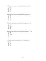
4. The given points are plotted on the graph below:

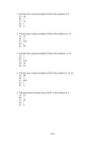
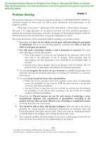
1. The given points are plotted on the graph below:
9
8
7
6
5
4
3
2
1
-9 -8 -7

-6

-5

-4

-3 -2 -1

-1

(-2, -1)
-2
(-1, -2)-3
-4
-5
-6
-7
-8
-9

(3,5)

(-2,5)

(6,1)
0

1

2

3

4

5

6

7


x
8

9

-9

2. The given points are plotted on the graph below:

-8 -7

-6

-5

-4

(-2,0)
-6

-5

-4

-3 -2 -1

-9 -8 -7

-6


-5

-4

-3 -2 -1

x

0 1 2
-1
-2 (0,-2)
-3
-4
-5
-6
-7
-8
-9

3

4

5

6

7


8

9

-9 -8 -7

-1
-2
-3
-4
-5
-6
-7
-8
-9

-6

-5

-4

-3 -2 -1

(-1,-4)

(5,0)
1

1


(6,0)
2

3

4

5

6

x
7

8

9

2

3

4

5

9
8
7

6
(0,5)5
4
3
2
1

x
6

7

8

9

-9 -8 -7

-6

-5

-4

-3 -2 -1

(-3,-2)
(4,-3)

Full file at />

-1
-2
-3
-4
-5
-6
-7
-8
-9

0

1

(4.5,2.5)

x
2

3

4

5

6

7

8


9

6. The given points are plotted on the graph below:

y

0

-1
-2
-3
-4
-5
-6
-7
-8
-9
-10

0

9
8
7
6
(-1/2,5) 5
4
3
2

1 (0,0.5)

(4,4)

3. The given points are plotted on the graph below:

(-7,1)

-1

y

9
8
7
6 (0,6)
5
4
3
2
1

9
8
7
6
5
4
3
2

1

-3 -2

(4,2)

5. The given points are plotted on the graph below:

y

-9 -8 -7

10 y
9
8
7
6 (0,
(0,6)
6)
5
4
3
2
1

y

-1
-2
-3

-4
-5
-6
-7
-8
-9

y

(3/4,4)

x
0

1

2

3

(3,-5)

4

5

6

7


8

9


Solution Manual for Finite Mathematics An Applied Approach 3rd Edition by Young
Full file at />2 Chapter 1 Applications of Linear Functions
10. The coordinates are shown next to the appropriate point
in the graph below:

7. The given points are plotted on the graph below:
9
8
7
6
5
4
3
2
(0,0) 1
-9 -8 -7

-6

-5

-4

-3 -2 -1


-1
-2
-3
-4
-5
-6
-7
-8
-9

y

(4,1/2)
0

1

2

3

4

(-1,3)

x

(4,0)
5


6

7

8

10 y
9
8
7
6
5 (0,5)
4
3
2
1

(-4,2)

9

(4,-0.5)

-9

-8 -7

-6

-5


-4

-3 -2

(-4,-3)

-1

0

1

(5,1)

x
2

-1
-2 (0,-2)
-3
-4
(2,-4)
-5
-6
-7
-8
-9
-10


3

4

5

6

7

8

9

8. The given points are plotted on the graph below:
11. The data is shown below:
y

9
8
7
6
5
4 (0,4.5)
3
2
1

-9 -8 -7


-6

-5

-4

-3 -2 -1

-1
-2
-3
(-2,-3) -4
-5
-6
-7
-8
-9

0

1

1050

x

2

3


4

5

6

7

8

9

(3,-4)

Dollars (billions)

(-3.5,0.5)

U.S. Exports

950

1996

9. The coordinates are shown next to the appropriate point
in the graph below:

(-3,3)

-9


-8 -7

-6

-5

-4

-3 -2

-1

-1
-2
-3
(-2,-3) -4
-5
-6
-7
-8
-9
-10

1997

1998

2000 Year


1999

12. The data is shown below:

y

Civilian Labor Forces
80

(1,2)
(4,0)
0

1

2

3

4

x
5

6

7

8


(2,-2)

9

U.S. Males (millions)

10
9
8
7
6
5
4
3
2
1

1000

70

60

50

Females (millions)
40

Full file at />
30


40

50

60


Solution Manual for Finite Mathematics An Applied Approach 3rd Edition by Young
Full file at />Section 1.1 The Cartesian Plane and Graphing
16. The data is shown below:

13. The data is shown below:

Gestation Periods vs Life Span

30

20

10

Gestation (days)
300

400

500

600


x

% of U.S. High School Graduates

Life Span (years)

40

200

College Enrollment

70

50

68
66
64
62
60
58

Year

56
1989 1990 1991 1992 1993

1994 1995 1996 1997 1998


17. The Data is shown below:
14. The data is shown below:

Median Household Income

Daily English Newspapers
1400

Median income

37500

Evening

1200

1000

35000
32500
30000

800

1988
400

500


600

700

1990

1992

1996

1994

18. Recognizing that the equation is a linear equation, we
simply need to find two points on the line. So we will
create a representative table using any two values of x we
wish to use.

15. The data is shown below:

U.S. Smokers
% of Smokers (18 and older)

50

45

x

y


0

2(0) − 3 = −3

3
2

40

2 ( 32 ) − 3 = 0

( x, y )
(0, −3)

(

3
2

, 0)

The graph is shown at the top of the next page.

35

30

25

Year

20

1965

1970

1975

1980

1998

Morning

1985

1990

1995

Full file at />
3


Solution Manual for Finite Mathematics An Applied Approach 3rd Edition by Young
Full file at />4 Chapter 1 Applications of Linear Functions
Plotting the points and connecting them with a smooth
curve we see the following graph:
y


9
8
7
6
5
4
3
2
1
-9 -8 -7

-6

-5

-4

-3 -2 -1

1

-1
-2
-3
-4 (0,-3)
-5
-6
-7
-8
-9


2

3

9
8
7
6
5
4
3
2
1

x

(1.5,0)
0

4

5

6

7

8


9

-9 -8 -7

19. Recognizing that the equation is a linear equation, we
simply need to find two points on the line. So we will
create a representative table using any two values of x we
wish to use.

-6

-5

-4

-3 -2 -1

-1
-2
-3
-4
-5
-6
-7
-8
-9

y

x


(0,0)
0

1

2

3

4

5

6

( x, y )

x

y

0

0 − 4 = −4

−1

5 ( −1) = −5


4

4−4 = 0

( 0, −4)
( 4, 0)

( x, y )

( −1, −5)
(1,5)

-8 -7

-6

-5

-4

-3 -2

-1

(4,0)
1

-1
-2
-3

-4
-5 (0,-4)
-6
-7
-8
-9
-10

2

3

5

6

7

8

9

y

( x, y )

0

−2 ( 0 ) = 0


( 0, 0)
( 2, −4)

−2 ( 2) = −4

9
8
7
6
5
4
3
2
1
-9 -8 -7

-6

-5

-4

-3 -2 -1

(-1,-5)

x

Full file at />
9


Plotting the points and connecting them with a smooth
curve we see the following graph:

x
4

20. Recognizing that the equation is a linear equation, we
simply need to find two points on the line. So we will
create a representative table using any two values of x we
wish to use.

2

5 (1) = 5

1

y

0

8

21. Recognizing that the equation is a linear equation, we
simply need to find two points on the line. So we will
create a representative table using any two values of x we
wish to use.

y


10
9
8
7
6
5
4
3
2
1

7

(2,-4)

x

Plotting the points and connecting them with a smooth
curve we see the following graph:

-9

Plotting the points and connecting them with a smooth
curve we see the following graph:

-1
-2
-3
-4

-5
-6
-7
-8
-9

y

(1,5)

x
0

1

2

3

4

5

6

7

8

9


22. Recognizing that the equation is a linear equation, we
simply need to find two points on the line. So we will
create a representative table using any two values of x we
wish to use.

x

y

( x, y )

0

2 ( 0) − 6 = −6

( 0, −6)
( 3, 0)

3

2 ( 3) − 6 = 0


Solution Manual for Finite Mathematics An Applied Approach 3rd Edition by Young
Full file at />Section 1.1 The Cartesian Plane and Graphing
Plotting the points and connecting them with a smooth
curve we see the following graph:
9
8

7
6
5
4
3
2
1
-9 -8 -7

-6

-5

-4

-3 -2 -1

Plotting the points and connecting them with a smooth
curve we see the following graph:

y

(3,0)
0

1

-1
-2
-3

-4
-5
-6
-7 (0,-6)
-8
-9

2

9
8
7
6
5
4
3
2
1

x
3

4

5

6

7


8

9

-9 -8 -7

23. Recognizing that the equation is a linear equation, we
simply need to find two points on the line. So we will
create a representative table using any two values of x we
wish to use.

-6

-5

-4

-3 -2 -1

-1
-2
-3
-4
-5
-6
-7
-8
-9

y


x
0

1

2

3

4

5

6

y

( x, y )

x

y

( x, y )

0

−2 ( 0 ) + 7 = 7


( 0, 7)
( 3,1)

−5

( −5 ) + 5 = 0
( 0) + 5 = 5

( −5, 0)
( 0,5)

−2 ( 3) + 7 = 1

0

Plotting the points and connecting them with a smooth
curve we see the following graph:
9
8
7
6
5
4
3
2
1
-9 -8 -7

-6


-5

-4

-3 -2 -1

-1
-2
-3
-4
-5
-6
-7
-8
-9

2

3

4

5

6

7

8


9

24. Recognizing that the equation is a linear equation, we
simply need to find two points on the line. So we will
create a representative table using any two values of x we
wish to use.

y

( x, y )

( 0) + 2 = 2
−1
2 ( 4) + 2 = 0

( 0, 2)
( 4, 0)

x

0

4

−1
2

-9

-8 -7


-6

-5

-4

-3 -2

-1

-1
-2
-3
-4
-5
-6
-7
-8
-9
-10

0

1

x
2

3


4

5

6

7

8

9

26. Because the exponent on the variable is one, this is a
linear function. Therefore, we only need to plot two points.
Notice the representative table below:

x

f ( x) = 3 x − 1

0

f ( 0) = 3 ( 0) − 1 = −1

2

f ( 2) = 3 ( 2) − 1 = 5

The graph is shown at the top of the next page.


Full file at />
9

10 y
9
8
7
6
5
4 (0,5)
3
2
1

(-5,0)

x
1

8

Plotting the points and connecting them with a smooth
curve we see the following graph:

y

0

7


25. Recognizing that the equation is a linear equation, we
simply need to find two points on the line. So we will
create a representative table using any two values of x we
wish to use.

x
3

5

( x, f ( x ) )
( 0, −1)
( 2,5)


Solution Manual for Finite Mathematics An Applied Approach 3rd Edition by Young
Full file at />6 Chapter 1 Applications of Linear Functions
Plotting the points in the plane and connecting them with a
smooth curve we see the following graph:
9
8
7
6
5
4
3
2
1
-9 -8 -7


-6

-5

-4

-3 -2 -1

f(x)

f(t)

x
0

1

-1
-2 (0,-1)
-3
-4
-5
-6
-7
-8
-9

2


3

4

5

x

f ( x) = −2 x

−1

f ( −1) = −2 ( −1) = 2

6

7

8

9

-9 -8 -7

( x, f ( x ) )
( −1, 2)
( 2, −4)

f ( 2 ) = −2 ( 2 ) = − 4


Plotting the points in the plane and connecting them with a
smooth curve we see the following graph:
9
8
7
6
5
4
3
2
1
-9 -8 -7

-6

-5

-4

-3 -2 -1

-1
-2
-3
-4
-5
-6
-7
-8
-9


9
8
7
6
5
(0,4)
4
3
2
1

(2,5)

27. Because the exponent on the variable is one, this is a
linear function. Therefore, we only need to plot two points.
Notice the representative table below:

2

Plotting the points in the plane and connecting them with a
smooth curve we see the following graph:

f(x)

x
0

1


2

3

4

5

6

7

8

9

-6

-5

-4

-3 -2 -1

f (t ) = −t + 4

0

f ( 0) = − ( 0) + 4 = 4


4

f ( 4) = − ( 4) + 4 = 0

( t , f ( t ))
( 0, 4)
( 4, 0)

Full file at />
(4,0)
2

3

4

5

t
6

7

8

9

( t , P ( t ))

t


P (t ) = t 2 − 3

−2

P ( −2) = ( −2) − 3 = 1

−1

P ( −1) = ( −1) − 3 = −2

0

P ( 0 ) = ( 0 ) − 3 = −3

1

P (1) = (1) − 3 = −2

2

P ( 2) = ( 2) − 3 = 1

( −2,1)

2

( −1, −2)
( 0, −3)
(1, −2)

( 2,1)

2

2

2

2

Plotting the points in the plane, and connecting them we a
smooth curve, we graph the parabola.

(-2,1)

t

1

29. The exponent on the independent variable is two, the
graph will be a parabola. We need to plot several points to
get the basic shape. To do this we will simply choose more
values of t . However, we still create the same
representative table below:

-9 -8 -7

28. Because the exponent on the variable is one, this is a
linear function. Therefore, we only need to plot two points.
Notice the representative table below:


-1
-2
-3
-4
-5
-6
-7
-8
-9

0

-6

-5

-4

-3 -2 -1

9
8
7
6
5
4
3
2
1


P(t)

t

(2,1)

0 1 2 3
-1
-2
(-1,-2) -3
(1,-2)
-4
(0,-3)
-5
-6
-7
-8
-9

4

5

6

7

8


9


Solution Manual for Finite Mathematics An Applied Approach 3rd Edition by Young
Full file at />Section 1.1 The Cartesian Plane and Graphing
30. Once again, looking at the exponent on the independent
variable, we see that it is a one. This is a linear equation,
and we only need to plot two points. The representative
table is as follows:

p

Q ( p) = 2 p − 4

0

Q ( 0) = 2 ( 0) − 4 = −4

( 0, −4)
( 2, 0)

Plotting the appropriate points and connecting the plots with
a smooth curve, we get the graph of the line below:
9
8
7
6
5
4
3

2
1
-9 -8 -7

-6

-5

-4

-3 -2 -1

For Problems 32–37, I will be using the standard graphing
window on the calculator.

( p, Q ( p ) )

Q ( 2) = 2 ( 2) − 4 = 0

2

Q(p)

(2,0)

32. Entering y =
following graph:

x 2 into the graphing calculator, shows the


p

0 1 2
-1
-2
-3
-4
-5 (0,-4)
-6
-7
-8
-9

3

4

5

6

7

8

9

33. Entering y = x + 1 into the graphing calculator,
shows the following graph:
2


31. Once again, we have a linear function. The
representative table is shown below:

p

Z ( p) = p − 1

−2

Z ( −2) = ( −2) − 1 = −3

( p, Z ( p ) )
( −2, −3)
( 5, 4)

Z ( 5) = ( 5 ) − 1 = 4

5

Plotting the points and connecting them with a smooth
curve, we see the graph of the line below:
9
8
7
6
5
4
3
2

1
-9 -8 -7

-6

-5

-4

-3 -2 -1

(-2,-3)

-1
-2
-3
-4
-5
-6
-7
-8
-9

Z(p)

(5,4)

p
0


1

2

3

4

5

7

6

7

8

Full file at />
9

34. Entering y = x − 2 into the graphing calculator,
shows the following graph:
2


Solution Manual for Finite Mathematics An Applied Approach 3rd Edition by Young
Full file at />8 Chapter 1 Applications of Linear Functions
35. Entering y = x − 6 into the graphing calculator,
shows the following graph:


t

f (t )

0

0
f ( 0) = 50 (1 − 120
) = 50

( t , f ( t ))
( 0,50)
( 60, 25)
(120, 0)

60
f ( 60) = 50 (1 − 120
) = 25

60

f (120) = 50 (1 − 120
120 ) = 0

120

Plotting these arbitrary points and connecting them with a
smooth curve, we see the graph of the function:
f(t) (pollutant in ppm)


36. Entering y = x into the graphing calculator, shows
the following graph:

60

3

50 (0,50)

40

30

(60,25)

20

10

t (days)
0

20

40

60

80


100

120

(120,0)

37. Entering

y = ( x − 1) into the graphing calculator,
3

shows the following graph:

39. The independent variable in this function is thousands
of miles x . This application implies that x ≥ 0 . It also
would not make sense to have a negative tread depth, so

f ( x ) ≥ 0 . This implies that (1 − 40x ) ≥ 0 ⇒ x ≤ 40 . So

an appropriate domain for this function would be
0 ≤ x ≤ 40 . Creating a representative table using
appropriate values from the domain we see:

38. The independent variable in this case is time, t . We
would believe that time cannot be negative so the minimum
value is 0, the time the removal process began. It would
also make sense that there could not be a negative amount
of pollutant. So f (t ) ≥ 0 . Which means


(1 − ) ≥ 0 ⇒ t ≤ 120 . So an appropriate domain for
t
120

this application would be 0 ≤ t ≤ 120 . Now create a
representative table like the one shown at the top of the next
column.

Full file at />
x

f ( x)

0

f ( 0) = 2 (1 − 400 ) = 2

20

40

f ( 20) = 2 (1 − 20
40 ) = 1

f ( 40) = 2 (1 − 40
40 ) = 0

The graph is shown at the top of the next page.

( x, f ( x ) )

( 0, 2)
( 20,1)
( 40, 0)


Solution Manual for Finite Mathematics An Applied Approach 3rd Edition by Young
Full file at />Section 1.1 The Cartesian Plane and Graphing
Plotting the points from the previous page and connecting
them with a smooth curve gives us the graph of the
function:

p in hundreds of
dollars. Since price must be positive, p ≥ 0 . It also makes

41. The independent variable is price

sense to have a positive number of stereos sold. This means

(

that 16 −

f(x)
(tread depth in cm's)

p2
4

) ≥ 0 ⇒ −8 ≤ p ≤ 8 . However since price


is positive, and appropriate domain would be 0 ≤
Create a representative table:

4

9

p ≤8.

3

2

(40,0)
10

S ( p ) = 30 16 −

20

30

40

Plotting the points and connecting them with a smooth
curve we get the graph of the function:
500

representative table using appropriate points from the
domain:


400

( p, S ( p ) )

0

S ( 0) = 25 − ( 0) = 25

1

S (1) = 25 − (1) = 24

3

S ( 3) = 25 − ( 3) = 16

5

S ( 5) = 25 − ( 5) = 0

( 0, 25)
(1, 24)
( 3,16)
( 5, 0)

2

2


2

2

Plotting the points and connecting them with a smooth
curve we see the graph of the function:
28

S(p) (thousands of DVD's)

26 (0,25)

S(p) (# of steroes sold each year)

22

300

(6,210)

200

100

(8,0)
0

(3,16)

4


5

6

7

8

p (100's of dollars)
9

10

11

0

C ( 0) = 500 + 120 ( 0) = 500

10
25

8

3

C ( x)

12

10

2

x

16
14

1

12

13

C (10) = 500 + 120 (10) = 1700

C ( 25) = 500 + 120 ( 25) = 3500

6

The graph is shown at the top of the next page.

4
2

p (dollars)

(5,0)
0


1

2

3

4

5

6

Full file at />
14

42. The independent variable in this application is the
number of inspections during one week x . Since there are
only five inspectors the maximum number of inspections in
a given week is 25. So an appropriate domain for this
function is 0 ≤ x ≤ 25 . Create a representative table:

20
18

(2,450)

(0,480)

(1,24)


24

(8, 0)

82
4

p.

25 − p 2 ≥ 0 ⇒ −5 ≤ p ≤ 5 . However since p ≥ 0 , we
establish the appropriate domain of 0 ≤ p ≤ 5 . Create a

S ( p)

( 2, 450)
( 6, 210)

62
4

8

p

( 0, 480)

22
4


6

Thus it makes sense that p ≥ 0 . Likewise, the number of
DVD’s sold must be positive. This means that

( p, S ( p ) )

2

50

40. The independent variable in this problem is price

)

( )
S ( 2) = 30 (16 − ) = 450
S ( 6) = 30 (16 − ) = 210
S (8) = 30 (16 − ) = 0

2

x (1000's of miles)

p2
4

S ( 0) = 30 16 − 04 = 480

0


(20,1)
1

0

(

p

(0,2)

( x, C ( x ) )
( 0,500)

(10,1700)
( 25,3500)


Solution Manual for Finite Mathematics An Applied Approach 3rd Edition by Young
Full file at />10 Chapter 1 Applications of Linear Functions
Plotting the points and connecting them with a smooth
curve, we get the graph of the function:

b. The graph is:
9
8
7
6
5

4
3
2
1

C(x) (cost in dollars)
(25,3500)
3000

-9 -8 -7

-6

-5

-4

-3 -2 -1

2000

(10,1700)
1000

(0,500)

-1
-2
-3
-4

-5
-6
-7
-8
-9

y

(4,5)

x
0

1

2

3

4

5

6

7

8

9


(6,-1)

x (# of inspections)
0

5

10

15

20

25

2.
43. The independent variable in this application is the
number of shifts needed each week x . Since there are
eight students available to work one shift a day, there is a
maximum number of 40 shifts per week. The appropriate
domain for this function is 0 ≤ x ≤ 40 .

a. The slope is m =

−1 − (−1) 0
=
=0
−2 − 3
−5


b. The graph is:
9
8
7
6
5
4
3
2
1

Create a representative table using appropriate points from
the domain.

x

C ( x ) = 80 + 40 x

0

C ( 0) = 80 + 40 ( 0) = 80

( x, C ( x ) )
( 0,80)

C ( 20) = 80 + 40 ( 20) = 880

20


-6

-5

-4

( 20,880)

C ( 40) = 80 + 40 ( 40) = 1680

40

-9 -8 -7

( 40,1680)

Plotting the points and connecting them with a smooth
curve, we get the graph of the function:

-3 -2 -1

-1
(-2,-1) -2
-3
-4
-5
-6
-7
-8
-9


3.

C(x) (cost in dollars)
(40,1680)

1500

a. The slope is

m=

y

x
0

1

2

3

4

5

6

7


8

9

5

6

7

8

9

(3,-1)

5−5
0
= −4 = 0
1
−1 − 3
3

b. The graph is:
1000

9
8
7

6
5
(-1,5) 4
3
2
1

(20,880)
500

x (# of shifts)

(0,80)
0

5

10

15

20

25

30

35

40


45

Exercises Section 1.2
1.
a. The slope is m =

−1 − 5 −6
=
= −3
6−4
2

Full file at />
-9 -8 -7

-6

-5

-4

-3 -2 -1

-1
-2
-3
-4
-5
-6

-7
-8
-9

y

(1/3,5)

x
0

1

2

3

4


Solution Manual for Finite Mathematics An Applied Approach 3rd Edition by Young
Full file at />Section 1.2 Equations of Straight Lines
b. The graph is:

4.

−1 − 0 −1 1
a. The slope is m =
=
=

−2 − 0 −2 2

280
260
240
220
200
180
160
140
120
100
80
60
40
20

b. The graph is:
9
8
7
6
5
4
3
2
1
(0,0)
-9 -8 -7


-6

-5

-4

-3 -2 -1

-1

y

-8

x

0

1

2

3

4

5

6


7

8

-6

-4

-2

9

(-2,-1) -2
-3
-4
-5
-6
-7
-8
-9

7.
a. The slope is m =

5.

-20
-40
-60
-80


-6

-5

-4

-3 -2 -1

10
9
8
7
6
5
4
3
2
1

-1
-2
-3
-4
-5
-6
-7
-8
-9


y

(1,5.8)
-9

-6

-5

-4

-3 -2

x
1

2

3

4

5

6

7

8


6.
a. The slope is

m=

-8 -7

(7/8,3.7)

0

(1.6,250)

(2.9,123)

x
0

2

4

6

8

5 − ( −2 ) 7
= = No Slope
3− 3
0


b. The graph is:

-9 -8 -7

y

b. The graph is:

5.8 − 3.7 2.1
= 1 = 16.8
a. The slope is m =
1 − 78
8
9
8
7
6
5
4
3
2
1

11

9

8.
a. The slope is m =


-1

-1
-2
-3
-4
-5
-6
-7
-8
-9
-10

(3,5)

x
0

1

2

3

4

5

6


7

8

9

(3,-2)

8−3 5
= =5
7−6 1

b. The graph is:
9
8
7
6
5
4
3
2
1

123 − 250 −127 −1270
9
=
=
= −97
2.9 − 1.6

1.3
13
13

-9 -8 -7

Full file at />
y

-6

-5

-4

-3 -2 -1

-1
-2
-3
-4
-5
-6
-7
-8
-9

y
(7,8)


(6,3)

x
0

1

2

3

4

5

6

7

8

9


Solution Manual for Finite Mathematics An Applied Approach 3rd Edition by Young
Full file at />12 Chapter 1 Applications of Linear Functions
y = −2 x + 9
2 x + y = −2 x + 9 + 2 x

9.


3 −1 2
a. The slope is m =
= =1
3 −1 2

General Form: 2 x + y = 9

b. The graph is:
10
9
8
7
6
5
4
3
2
1
-9

-8 -7

-6

-5

-4

-3 -2


10.
a. The slope is m =

-1

-1
-2
-3
-4
-5
-6
-7
-8
-9
-10

y

b. The graph is shown below:

(3,3)

x

(1,1)
0

1


2

3

4

5

6

7

8

9

-9 -8 -7

2−2
0
=
=0
6 − ( −4) 10

(-4,2)

-9 -8 -7

-6


-5

-4

-3 -2 -1

-1
-2
-3
-4
-5
-6
-7
-8
-9

y

-5

-4

-3 -2 -1

-1
-2
-3
-4
-5
-6

-7
-8
-9

(2,5)

x
0

1

2

3

4

5

6

7

8

9

y − 6 = 4 ( x − ( −4)) .
(6,2)


Now solve for

y to get the slope-intercept form:

x
0

1

2

3

4

5

6

7

8

9

11.
a. To begin with we will use point-slope to find the slopeintercept form of the line. Substituting the appropriate slope
and coordinates we see the equation: y − 5 = −2( x − 2) .
Now solve for y to get the slope-intercept form.


y − 5 = −2 x + 4
y − 5 + 5 = −2 x + 4 + 5
Slope-intercept Form:

-6

y

12.
a. To begin with we will use point-slope to find the slopeintercept form of the line. Substituting the appropriate slope
and coordinates we see the equation:

b. The graph is:
9
8
7
6
5
4
3
2
1

9
8
7
6
5
4
3

2
1

y = −2 x + 9

Once the slope-intercept form of the line is known, we
isolate the constant term to get the general form of the line.
Do this by subtracting the x term from both sides of the
equation.

Full file at />
y − 6 = 4 x + 22
y − 6 + 6 = −4 x + 16 + 6
Slope-intercept Form: y = 4 x + 22
Once the slope-intercept form of the line is known, we
isolate the constant term to get the general form of the line.
Do this by subtracting the x term from both sides of the
equation.

y = −4 x − 10
4 x + y = −4 x − 10 + 4 x
General Form:

4 x + y = −10

b. The graph is shown at the top of the next page.


Solution Manual for Finite Mathematics An Applied Approach 3rd Edition by Young
Full file at />Section 1.2 Equations of Straight Lines

10
9
8
7
6
5
4
3
2
1

(-4,6)

-9

-8 -7

-6

-5

-4

-3 -2

-1

-1
-2
-3

-4
-5
-6
-7
-8
-9
-10

y

14.
a. To begin with we will use point-slope to find the slopeintercept form of the line. Substituting the appropriate slope
and coordinates we see the equation:
x

0

1

2

3

4

5

6

7


8

2
3

y − 0 = −12( x − 4) .

9

Now solve for y to get the slope-intercept form.

y = −12 x + 48
Slope-intercept Form: y = −12 x + 48

13.
a. To begin with we will use point-slope to find the slopeintercept form of the line. Substituting the appropriate slope
and coordinates we see the equation:

y − 5.7 =

13

( x − 0) .

Once the slope-intercept form of the line is known, we
isolate the constant term to get the general form of the line.
Do this by subtracting the x term from both sides of the
equation.


y = −12 x + 48
12 x + y = −12 x + 48 + 12 x

Now solve for y to get the slope-intercept form.
General Form:

y − 5.7 = 23 x
y − 5.7 + 5.7 = 23 x + 5.7
Slope-intercept Form: y =

12 x + y = 48

b. The graph is shown below:
2
3

9
8
7
6
5
4
3
2
1

x + 5.7

Once the slope-intercept form of the line is known, we
isolate the constant term to get the general form of the line.

Do this by subtracting the x term from both sides of the
equation.

-9 -8 -7

-6

-5

-4

-3 -2 -1

y = 23 x + 5.7
− 23 x + y = 23 x + 5.7 − 23 x
General Form:

−2
3

x + y = 5.7 ⇒ −20 x + 30 y = 171

b. The graph is shown below:
y

-9 -8 -7

-6

-5


-4

-3 -2 -1

-1
-2
-3
-4
-5
-6
-7
-8
-9

0

1

x

(4,0)
0

1

2

3


4

5

6

7

8

9

15.
a. To begin, find the slope of the line passing through the
two points. m =

9
8
7
6
5 (0,5.7)
4
3
2
1

-1
-2
-3
-4

-5
-6
-7
-8
-9

y

−1 − 4 −5
=
. Now use point-slope to
6−3
3

find the slope-intercept form of the line. Substitute the
appropriate slope and one of the known coordinates to get
the equation:
x
2

3

4

5

6

7


8

Full file at />
y−4=

−5
3

( x − 3) .

9

We solve for y at the top of the next page to put the
equation in slope–intercept form.


Solution Manual for Finite Mathematics An Applied Approach 3rd Edition by Young
Full file at />14 Chapter 1 Applications of Linear Functions
y − 4 = −35 x + 5
y − 4 + 4 = −35 x + 5 + 4

Once the slope-intercept form of the line is known, we
isolate the constant term to get the general form of the line.
Do this by subtracting the x term from both sides of the
equation.

Slope-intercept Form: y =

−5
3


x+9

Once the slope-intercept form of the line is known, we
isolate the constant term to get the general form of the line.
Do this by subtracting the x term from both sides of the
equation as shown:

y = −35 x + 9
5
−5
5
3 x+ y = 3 x+9+ 3 x
General Form:

5
3

y = 74 x + 267
− 74 x + y = 74 x + 267 − 74 x
General Form:

-5

-4

(-3,2)

-3 -2 -1


-1
-2
-3
-4
-5
-6
-7
-8
-9

y

-9 -8 -7

-5

-4

-3 -2 -1

x
0

1

2

3

4


5

6

7

8

9

(6,-1)

26
7

⇒ −4 x + 7 y = 26

(1/2,4)

x
0

1

2

3

4


5

6

7

8

9

3 −1
−20
=
. Now use point-slope
−2 − 0.3 23

to find the slope-intercept form of the line. Substitute the
appropriate slope and one of the known coordinates to get
the equation shown at the top of the next column:

find the slope-intercept form of the line. Substitute the
appropriate slope and one of the known coordinates to get
the equation:

( x − 12 ) .

y −1 =

−20

23

( x − 0.3) .

Now solve for y to get the slope-intercept form.

y − 1 = −2320 x + 236
y − 1 + 1 = −2320 x + 236 + 1
Slope-intercept Form: y =

Now solve for y to get the slope-intercept form.

y − 4 = 74 x − 72
y − 4 + 4 = 74 x − 72 + 4
Slope-intercept Form: y =

-1
-2
-3
-4
-5
-6
-7
-8
-9

y

17.
a. To begin, find the slope of the line passing through the

two points. m =

2−4 4
two points. m =
= . Now use point-slope to
−3 − 12 7

4
7

-6

(3,4)

16.
a. To begin, find the slope of the line passing through the

y−4=

9
8
7
6
5
4
3
2
1

x + y = 9 ⇒ 5 x + 3 y = 27


9
8
7
6
5
4
3
2
1
-6

x+ y =

b. The graph is shown below:

b. The graph is shown below:

-9 -8 -7

−4
7

4
7

x + 267

x + 29
23


Once the slope-intercept form of the line is known, we
isolate the constant term to get the general form of the line.
Do this by subtracting the x term from both sides of the
equation.

y = −2320 x + 29
23
20
−20
29
20
23 x + y = 23 x + 23 + 23 x
General Form:

Full file at />
−20
23

20
23

x+ y =

29
23

⇒ 20 x + 23 y = 29



Solution Manual for Finite Mathematics An Applied Approach 3rd Edition by Young
Full file at />Section 1.2 Equations of Straight Lines

15

y
1200

b. The graph is shown below:

(-2,3)
-9 -8 -7

-6

-5

-4

-3 -2 -1

9
8
7
6
5
4
3
2
1

-1
-2
-3
-4
-5
-6
-7
-8
-9

y

1000

800

(20,700)

600

(0.3,1)
0

1

2

3

4


5

6

7

8

(10,500)

400

x
9

18.
a. To begin, find the slope of the line passing through the

700 − 500
= 20 . Now use point-slope
two points. m =
20 − 10
to find the slope-intercept form of the line. Substitute the
appropriate slope and one of the known coordinates to get
the equation:

y − 500 = 20( x − 10) .

200


x
-8 -6 -4

-2

0

2

4

6

8 10 12 14 16 18 20 22 24 26 28

19.
a. To begin, find the slope of the line passing through the
two points. m =

150 − 300
= −25 . Now use point-slope
23 − 17

to find the slope-intercept form of the line. Substitute the
appropriate slope and one of the known coordinates to get
the equation:

y − 300 = −25( x − 17) .
Now solve for y to get the slope-intercept form.


Now solve for

y to get the slope-intercept form.

y − 500 = 20 x − 200
y − 500 + 500 = 20 x − 200 + 500
Slope-intercept Form: y = 20 x + 300
Once the slope-intercept form of the line is known, we
isolate the constant term to get the general form of the line.
Do this by subtracting the x term from both sides of the
equation.

y = 20 x + 300
−20 x + y = 20 x + 300 − 20 x
General Form:

−20 x + y = 300

b. The graph is shown at the top of the next column.

Full file at />
y − 300 = −25 x + 425
y − 300 + 300 = −25 x + 425 + 300
Slope-intercept Form: y = −25 x + 725
Once the slope-intercept form of the line is known, we
isolate the constant term to get the general form of the line.
Do this by subtracting the x term from both sides of the
equation.


y = −25 x + 725
25 x + y = −25 x + 725 + 25 x
General Form: 25 x + y = 725


Solution Manual for Finite Mathematics An Applied Approach 3rd Edition by Young
Full file at />16 Chapter 1 Applications of Linear Functions
b. The graph is shown below:

9
8
7
6
5
4
3
2
1

y
1200

1000

800
-9 -8 -7

-6

-5


-4

-3 -2 -1

600

400

(17,300)

200

(23,150)

x
-8 -6 -4

-2

0

2

4

6

y


(3,0)

0 1 2
-1
-2
-3 (0,-2)
-4
-5
-6
-7
-8
-9

4

5

6

7

8

9

8 10 12 14 16 18 20 22 24 26 28

21.

(


)

a. Since the x-intercept is the point 1.6, 0 and the y-

20.

(

)

a. Since the x-intercept is the point 3, 0 and the y-

(

)

intercept is the point 0, −2 , the slope of the line passing
through the two points is m =

0 − ( −2) 2
= . Now use
3− 0
3

the slope-intercept form of the line to find the equation.
Substitute the appropriate slope and the y-intercept into the
equation:

y = ( 23 ) x + ( −2) .


Now solve for

x

3

Slope-intercept Form: y =

2
3

x−2

Once the slope-intercept form of the line is known, we
isolate the constant term to get the general form of the line.
Do this by subtracting the x term from both sides of the
equation.

y = 23 x − 2
− 23 x + y = 23 x − 2 − 23 x
−2
3

)

through the two points is m =

0 − ( 4.3) −43
=

. Now
1.6 − 0
16

use the slope-intercept form of the line to find the equation.
Substitute the appropriate slope and the y-intercept into the
equation:

y = ( −1643 ) x + ( 4.3) .

Now solve for y to get the slope-intercept form.

y to get the slope-intercept form.

General Form:

(

intercept is the point 0, 4.3 , the slope of the line passing

x + y = −2 ⇒ −2 x + 3 y = −6

Slope-intercept Form: y =

−43
16

43
x + 10


Once the slope-intercept form of the line is known, we
isolate the constant term to get the general form of the line.
Do this by subtracting the x term from both sides of the
equation.
43
y = −1643 x + 10
43
−43
43
43
16 x + y = 16 x + 10 + 16 x

General Form:

43
16

43
x + y = 10
⇒ 215 x + 80 y = 344

b. The graph is shown below:
y

9
8
7
6
5
(0,4.3)

4
3
2
1
(1.6,0)

b. The graph is shown at the top of the column.

-9 -8 -7

Full file at />
-6

-5

-4

-3 -2 -1

-1
-2
-3
-4
-5
-6
-7
-8
-9

0


1

2

3

x
4

5

6

7

8

9


Solution Manual for Finite Mathematics An Applied Approach 3rd Edition by Young
Full file at />Section 1.2 Equations of Straight Lines
22. The equation of the horizontal line is y = −6

The graph of each equation is shown below:

The equations of the vertical line is x = 3

9

8
7
6
5
4
3
2
1

23. The equation of the horizontal line is y = 4
The equation of the vertical line is x =

17

−1
2

24. The equation of the horizontal line is y = 200
The equation of the vertical line is x = −5.7

-9 -8 -7

-6

-5

-4

-3 -2 -1


25. The equation of the horizontal line is y = −8.6
The equation of the vertical line is x = 1.2
Note: There are many solutions to 26–31. The following
are arbitrary choices.
26. Parallel lines have the same slope, so simply change the
constant term in the equation to get a parallel equation.

-1
-2
-3
-4
-5
-6
-7
-8
-9

y
4x-7y=-56
4x-7y=-28

4x-7y=6
0

1

2

3


4

5

6

7

x
8

9

4x-7y=28

28. Parallel lines have the same slope, so simply change the
constant term in the equation to get a parallel equation.
Original line:

Original line: y = 5 x

y = −3x + 7
y = −3x − 3

y = 5 x − 20

Parallel Lines: y = −3 x + 2

Parallel Lines: y = 5 x + 15


y = −3x + 5

y = 5 x + 20

The graph of each equation is shown below:
The graph of each equation is shown below:
9
8
7
6
5
4
3
2
1

y=-3x-9

y

y=5x+20

-9 -8 -7

-6

-5

-4


9
8
y=5x+15
7
6
5
4
3
2
1

-3 -2 -1

-1
-2
-3
-4
-5
-6
-7
-8
-9

0

1

y=5x

y=5x-20


x
2

3

4

5

6

7

8

-9 -8 -7

-6

-5

-4

-3 -2 -1

9

y=-3x-15


-1
-2
-3
-4
-5
-6
-7
-8
-9

y

y=-3x+15

x
0

1

2

3

4

5

6

7


8

9

y=-3x+7

29. Parallel lines have the same slope, so simply change the
constant term in the equation to get a parallel equation.
27. Parallel lines have the same slope, so simply change the
constant term in the equation to get a parallel equation.
Original line:

4x − 7 y = 6
4 x − 7 y = −56

Parallel Lines: 4 x − 7 y = −28

4 x − 7 y = 28

Full file at />
Original line: x = 5

x = −8
Parallel Lines: x = −4

x=2
The graph of each equation is shown at the top of the next
page.



Solution Manual for Finite Mathematics An Applied Approach 3rd Edition by Young
Full file at />18 Chapter 1 Applications of Linear Functions
x=-8

-9 -8 -7

x=-4

-6

-5

-4

-3 -2 -1

9
8
7
6
5
4
3
2
1
-1
-2
-3
-4

-5
-6
-7
-8
-9

y
x=2

x
0

1

2

3

4

5

6

7

8

9


-9 -8 -7

30. Parallel lines have the same slope, so simply change the
constant term in the equation to get a parallel equation.

y = −8
Parallel Lines: y = −4
y=3

-4

-3 -2 -1

-3 -2 -1

-1
-2
-3
-4
-5
-6
-7
-8
-9

-2x+4y=-3
0

1


2

3

4

5

6

7

8

x
9

-2x+4y=-25

-1
-2
-3
-4
-5
-6
-7
-8
-9

1

2

( x − 3)

Thus the equation parallel to the given line is:

y−5=

y
y=7

1
2

( x − 3) ⇒ y = 12 x + 72

33. The given line is in slope-intercept form y = −3 x − 7
Therefore the slope of the line is m1 = −3 . Find the
desired equation using point-slope form:

y=3

x
0

1

2

3


4

5

6

7

8

9

y − 2 = −3 ( x − 1.3)

y=-4

Thus the equation parallel to the given line is:
y=-8

31. Parallel lines have the same slope, so simply change the
constant term in the equation to get a parallel equation.
Original line:

-4

-2x+4y=16

32. Solve x − 2 y = 6 for y to find the slope of the line.


y−5=

9
8
7
6
5
4
3
2
1
-5

-5

-2x+4y=32

form:

The graph of each equation is shown below:

-6

-6

y

−2 y = − x + 6 ⇒ y = 12 x − 3 . Therefore the slope of the
line is m1 = 12 . Find the desired equation using point-slope


Original line: y = 7

-9 -8 -7

9
8
7
6
5
4
3
2
1

x=5

−2 x + 4 y = −3
−2 x + 4 y = −25

Parallel Lines: −2 x + 4 y = 16

−2 x + 4 y = 32
The graph of each equation is shown at the top of the next
column.

Full file at />
y − 2 = −3 x + 3.9 ⇒ y = −3 x + 5.9
34. Solve 2 x − 4 y = 7 for y to find the slope of the line.

−4 y = −2 x + 7 ⇒ y = 12 x − 74 .

Therefore the slope of the line is m1 =

1
2

. Find the desired

equation using point-slope form:

y − ( −3) =

1
2

( x − 12 )

Thus the equation parallel to the given line is:

y + 3 = 12 x − 14 ⇒ y = 12 x − 134


Solution Manual for Finite Mathematics An Applied Approach 3rd Edition by Young
Full file at />Section 1.2 Equations of Straight Lines
35. Solve 2 x + 3 y = 6 for y to find the slope of the line.

3 y = −2 x + 6 ⇒ y =

−2
3


x+ 2.

Therefore the slope of the line is m1 =

a. Since the equation is now in slope-intercept form, change
the coefficient on the x-term to create a line with the same
y-intercept.

y = −2 x + 2

−2
3

. Since the point

New equations: y = x + 2

y = 2x + 2

that we have is the y-intercept, find the desired equation
using slope-intercept form:

y=

−2
3

b. Change the y-coefficient of an equation in slope-intercept
form to find the equation of line that has the same xintercept.


x − 3.5

−y =

−3
2

x + 2 ⇒ y = 32 x − 2

New equations: 2 y =

−3
2

x+2⇒ y =

y=

−3
2

x + 2 ⇒ y = −3 x + 4

Thus the equation parallel to the given line is:

y=

−2
3


19

x − 3.5

1
2

36.
a. Since the equation is in slope-intercept form, change the
coefficient on the x-term to create a line with the same yintercept.

y = −2 x + 2

New equations: y = 4 x + 2

b. Change the y-coefficient of an equation in slope-intercept
form to find the equation of line that has the same xintercept.

−2 y = 2 x + 2 ⇒ y = − x − 1
New equations: 2 y = 2 x + 2 ⇒ y = x + 1
4 y = 2 x + 2 ⇒ y = 12 x + 12

37.
a. Since the equation is in slope-intercept form, change the
coefficient on the x-term to create a line with the same yintercept.

39. First solve the equation for y to put the equation in
slope-intercept form:

x − 2 y = 5 ⇒ y = 12 x − 52


y = −2 x − 52
New equations: y = − x −

New equations: y = x − 4

y = 2x − 4
b. Change the y-coefficient of an equation in slope-intercept
form to find the equation of line that has the same xintercept.

− y = −x − 4 ⇒ y = x + 4
−1
2

b. Change the y-coefficient of an equation in slope-intercept
form to find the equation of line that has the same xintercept.

− y = 12 x − 52 ⇒ y =
New equations:

38. First solve the equation for y to put the equation in
slope-intercept form:

3x + 2 y = 4 ⇒ y =

−3
2

x+2


Full file at />
−1
2
1
2

−1
2

x + 52

y = 12 x − 52 ⇒ y = − x + 5
y = 12 x − 52 ⇒ y = x − 5

40.
a. Since the equation is in slope-intercept form, change the
coefficient on the x-term to create a line with the same yintercept.

y = −2 x − 0.6
New equations: y = x − 0.6

y = 3.2 x − 0.6

x−2

y = − x − 4 ⇒ y = −2 x − 8

5
2


y = 5 x − 52

y = −2 x − 4

1
2

x +1

a. Since the equation is now in slope-intercept form, change
the coefficient on the x-term to create a line with the same
y-intercept.

y = 6x + 2

New equations: 2 y = − x − 4 ⇒ y =

−3
4

b. Change the y-coefficient of an equation in slope-intercept
form to find the equation of line that has the same xintercept.

− y = 1.3x − 0.6 ⇒ y = −1.3x + 0.6

New equations:

1
4
1

2

y = 1.3x − 0.6 ⇒ y = 5.2 x − 2.4
y = 1.3x − 0.6 ⇒ y = 2.6 x − 1.2


Solution Manual for Finite Mathematics An Applied Approach 3rd Edition by Young
Full file at />20 Chapter 1 Applications of Linear Functions
41. First solve the equation for y to put the equation in
slope-intercept form:

7 x + 6 y = 0 ⇒ y = 76 x
a, b. Notice that this line goes through the origin. That
means that the x-intercept and the y-intercept are the same
point. Therefore, simply change the x-coefficient to get the
new lines with the same x-intercept and y-intercept.

y = −2 x
New Equations: y = x

y = 2x
∆y
= m ⇒ ∆y = mi∆x (provided ∆x ≠ 0 ).
∆x
The slope of the line is m = 5 . So if:
42. Since

a. ∆x = 1 then ∆y = 5i1 = 5
b. ∆x = 2 then ∆y = 5i 2 = 10
c. ∆x = 5 then


∆y = 5i5 = 25

∆y
= m ⇒ ∆y = mi∆x (provided ∆x ≠ 0 ).
∆x
The slope of the line is m = 3 . So if:
43. Since

∆y = 3i1 = 3
b. ∆x = 2 then ∆y = 3i2 = 6
c. ∆x = 5 then ∆y = 3i5 = 15

a. ∆x = 1 then

∆y
= m ⇒ ∆y = mi∆x (provided ∆x ≠ 0 ).
∆x
The slope of the line is m = −6 . So if:
44. Since

a. ∆x = 1 then ∆y = −6i1 = −6
b. ∆x = 2 then ∆y = −6i2 = −12
c. ∆x = 5 then

∆y = −6i5 = −30

∆y
= m ⇒ ∆y = mi∆x (provided ∆x ≠ 0 ).
∆x

The slope of the line is m = −2 . So if:
45. Since

a. ∆x = 1 then ∆y = −2i1 = −2

∆y = −2i2 = −4
c. ∆x = 5 then ∆y = −2i5 = −10
b. ∆x = 2 then

Full file at />
∆y
= m ⇒ ∆y = mi∆x (provided ∆x ≠ 0 ).
∆x
The slope of the line is m = −21 . So if:
46. Since

a. ∆x = 1 then ∆y =

i1 = −21
b. ∆x = 2 then ∆y = i2 = −1
c. ∆x = 5 then ∆y = i5 = −25
−1
2
−1
2
−1
2

∆y
= m ⇒ ∆y = mi∆x (provided ∆x ≠ 0 ).

∆x
The slope of the line is m = −52 . So if:
47. Since

a. ∆x = 1 then ∆y =

i1 = −52
b. ∆x = 2 then ∆y = i2 = −54
c. ∆x = 5 then ∆y = i5 = −2
−2
5
−2
5
−2
5

∆y
= m ⇒ ∆y = mi∆x (provided ∆x ≠ 0 ).
∆x
The slope of the line is m = 12 . So if:
48. Since

a. ∆x = 1 then ∆y = 12 i1 =

1
2

b. ∆x = 2 then ∆y = 12 i2 = 1
c. ∆x = 5 then ∆y = 12 i5 =


5
2

49.
a.

S ( 5) = 800 ( 5) + 6000 = 10, 000
S ( 20) = 800 ( 20) + 6000 = 22, 000

The paper had 10,000 subscribers after five weeks, and
22,000 subscribers after 20 weeks.
b. Yes, the subscriptions are increasing by 800 subscriptions
per week (the slope of the linear function).
c. The slope is the number of new subscribers per week
after the start of the advertising campaign. The y-intercept
is the number of subscribers that were already subscribing
to the paper when the advertising campaign started.


Solution Manual for Finite Mathematics An Applied Approach 3rd Edition by Young
Full file at />Section 1.2 Equations of Straight Lines
d.

21

S(t) (Sales in $1000's)
26

S(t)


24

2500

Subscribers (in 1000's)

22
20

2000

18
16
1500

14
12
10

1000

8
6

500

4
2
-1 0 1 2 3 4 5 6 7 8
-2


t (Years since 1995)

t (weeks)
9 10 11 12 13 14 15 16 17 18 19

()

e. S t = 18, 000 ⇒ 800t + 6000 = 18, 000 Solve the

0

2

4

6

8

10

12

14

16

18


e. Three million is 3000 thousands so

linear equation by isolating the variable.

S ( t ) = 3, 000 implies that 120t + 600 = 3000 .

800t + 6000 = 18, 000
800t = 12, 000 ⇒ t = 15

Solve this equation for t :

120t + 600 = 3000 ⇒ 120t = 2400 ⇒ t = 20

It will take 15 weeks for subscriptions to reach 18,000.
50.
a. Since 1995 is the year where t = 0 , then 2000
corresponds to the year t = 5 and 2010 corresponds to the
year t = 15 . Substituting the appropriate value of t into
the function we see:

S ( 0) = 120 ( 0) + 600 = 600

S ( 5) = 120 ( 5) + 600 = 1200

S (15) = 120 (15) + 600 = 2400

The company expects to reach three million dollars in sales
in the year 2015.
51.
a. Since August 31st corresponds to t = 0 , September 15th

corresponds to t = 15 and September 20th corresponds to
t = 20 . Substitute the appropriate values of t into the
function.

P (15) = −2 (15) + 100 = 70

P ( 20) = −2 ( 20) + 100 = 60

Haworth Motorcycle Company had 600,000 dollars worth
of sales in 1995, 1,200,000 dollars worth of sales in 2000,
and is predicting 2,400,000 dollars worth of sales in 2010.

The agent predicts that there will be 70,000 grasshoppers
per acre on September 15th, and 60,000 grasshoppers per
acre on September 20th.

b. Yes, sales are increasing by 120,000 dollars each year
(The slope of the sales function).

b. According to the model, the grasshopper population is
decreasing by 2 thousand grasshoppers per acre each day.

c. The slope is the yearly increase in sales from the previous
year. The y-intercept is the total sales in 1995.

c. The slope of the graph is the rate in which the population
of grasshoppers per acre is decreasing each day. The yintercept is the estimated population of grasshoppers per
acre that were present on August 31st.

d. The graph is shown at the top of the next column.


d. The domain of this function is 0 ≤ t ≤ 50 because for
values of t larger than fifty, the estimated population of
grasshoppers is negative.
The graph of the function on this domain is shown at the top
of the next page.

Full file at />

Solution Manual for Finite Mathematics An Applied Approach 3rd Edition by Young
Full file at />P(t) (in 1000's per acre)

20

100

18

P(t) (1000's of ppm)

16
80

Water Pollutant

Grasshopper Population

22 Chapter 1 Applications of Linear Functions

60


40

20

14
12
10
8
6
4
2

t (Years since 1997)

t (days since 8/31)
0

5 10 15

20

25 30

35

40 45

50


55 60

65

0

70 75

2

4

6

8 10 12 14 16 18 20 22 24 26 28 30 32

-2

e. Since P (t ) = 20 ⇒ −2t + 100 = 20 , solve the linear
equation for t . −2t + 100 = 20 ⇒ 2t = 80 ⇒ t = 40
It will take 40 days for the grasshopper population to reach
20,000 per acre.

e. Since P (t ) = 0 ⇒ −800t + 18, 000 = 0 , solve the
linear equation for t .

−800t + 18, 000 = 0 ⇒ 800t = 18, 000 ⇒ t = 22.5

52.
a. Since 1997 corresponds to t = 0 , 1999 corresponds to

t = 2 , 2000 corresponds to t = 3 , and 2006 corresponds to
t = 9 . Substitute the appropriate values of t into the
function.

This means that the pollution will be completely gone from
the lake midway through the year 2019.

P ( 2) = −800 ( 2) + 18, 000 = 16, 400

for each increase of 1° Fahrenheit.

P ( 3) = −800 ( 3) + 18, 000 = 15, 600

P ( 9) = −800 ( 9) + 18, 000 = 10,800
According to the model, in 1999 there were 16,400 parts per
million (ppm) of this pollutant. In 2000 there were 15,600
ppm of this pollutant. It is estimated that there will be 10800
ppm of this pollutant in 2006.
b. Yes, the pollutant is decreasing each year by 800 parts
per million.
c. The slope is amount of the pollutant in parts per million
that is eliminated from the lake each year. The y-intercept
is the amount of the pollutant in parts per million in 1997.
d. The appropriate domain for this function is
0 ≤ t ≤ 22.5 . The graph of the function is shown at the
top of the next column.

53.
a. The corresponding rise in temperature will be 59 ° Celsius


b. C =

5
9

(80) − ( 1609 ) = 26 23 . The corresponding Celsius

temperature will be 26 23 ° ≈ 26.67° Celsius.
c. The original equation is C =

( )F −( ).
5
9

160
9

9C = 5 F − 160
9C + 160 = 5 F
9
9
5 C + 32 = F ⇒ F = 5 C + 32
d. The corresponding rise in temperature will be 95 °

Fahrenheit for each increase of 1° Celsius

54.
a. The independent variable is the number of miles driven.
So the domain must be positive. Moreover, the depth of the
tread on the tire must be positive as well.

Using this information the proper domain
is 0 ≤ x ≤ 40, 000 . The graph is shown at the top of the
next page.

Full file at />

Solution Manual for Finite Mathematics An Applied Approach 3rd Edition by Young
Full file at />Section 1.2 Equations of Straight Lines
T(x)

56.
a. The graph is shown below:

0.8
30
0.6

0.4

0.2

x (1000's of miles)
0

5

10

15


20

25

30

35

40

45

50

55

-0.2

b. From the graph we see that the he tread depth on a new
tire is one-half inch deep (y-intercept)
c. From the graph we see that the tread will last 40,000
miles until it is completely eliminated (depth is zero).
55.
a. The graph y = M ( x ) is shown below:

Male height (in cm's)

250

Median age of first-married men


Tread Depth (in inches)

1

23

28

A(x)

26
24
22
20
18
16
14
12
10
8
6
4
2

x (years since 1970)
0

5


10

15

20

25

b. Substitute x = 12 which corresponds to the year 1982

( )

( )

into the function. A 12 = 0.125 12 + 21.6 = 23.1
The median age for first-married men in 1982 was 23.1
years old.

M(x)

c.

0.125 x + 21.6 = 30 ⇒ .125 x = 8.4 ⇒ x = 67.2
0.125 x + 21.6 = 40 ⇒ .125 x = 18.4 ⇒ x = 147.2

200

150

The average age of first-married men will reach 30 of age in

the year 2037and reach 40 years of age in 2117.

100

50

Arm bone length (cm's) x
0

10

20

30

40

50

60

70

b. Substitute x = 46 in to the function.

M (46) = 2.9 ( 46) + 70.6 = 204 .
If a male measures 46 centimeters in length from elbow to
shoulder, then he is estimated to be 204 centimeters tall.
c. Now W ( x ) = 180 . Set the equation equal to 180 and
solve for x .


2.8 x + 71.5 = 180 ⇒ 2.8 x = 108.5 ⇒ x = 38.75
A female 180 centimeters tall, should measure 38.75
centimeters from elbow to shoulder.

This is not a realistic model over a long period of time,
because the average age will continue to increase. It would
be hard to imagine that the average age of first-married men
could be 100 years old (The year 2597 according to this
model).
57.
a. Substitute x = 11 which corresponds to the year 2006
into the function. S (11) = 0.91(11) + 28.96 = 38.97
In 2006, the company sales should reach 38,970 cases of
soft drinks.
b. Solve the equation 0.91x + 28.96 = 50 for x .

0.91x = 21.04 ⇒ x ≈ 23.12 .
Add this to 1995 to get the answer.
The company should reach 50,000 cases in sales in the year
2018 if this trend continues.
c. The graph is shown at the top of the next page.

Full file at />

Solution Manual for Finite Mathematics An Applied Approach 3rd Edition by Young
Full file at />24 Chapter 1 Applications of Linear Functions
S(x)

2. For a function to be linear, it must have a constant rate of

change. The decrease in yogurt outlets in the first year is 10,
followed by a decrease of 10 outlets in the second year, and
each year after that. Thus the rate of change for this relation
is constant each year. This relation is modeled by a linear
function.

Sales (in $1000's)

50

40

30

20

10

x (years since 1995)
0

5

10

15

20

25


58.
a. The graph is shown below for the appropriate values of
the domain:
10^4
10000

8000

Value (Dollars)

4. For a function to be linear, it must have a constant rate of
change. The decrease in yogurt outlets in the first year is
100
50
2 = 50 , followed by a decrease of 2 = 25 outlets in the
second year. Thus the rate of change for this relation is
decreasing each year. This relation is not modeled by a
linear function.

V(x)

5. For a function to be linear, it must have a constant rate of
change. The initial number of outlets is 60. The number of
outlets does not change after that, giving the relation a
constant rate of change of zero each year. This relation is
modeled by a linear function.

6000


4000

2000

x (years since 1995)
-1

3. For a function to be linear, it must have a constant rate of
change. The increase in yogurt outlets in the first year is 20,
followed by an increase of 20 outlets in the second year, and
each year after that. Thus the rate of change for this relation
is constant each year. This relation is modeled by a linear
function.

0

1

2

3

4

5

6

7


8

9 10 11 12 13 14 15

b. Substitute x = 4 into the function.

V (4) = −1333(4) + 12, 666 = 7334
The blue book value of the car would be 7,334 dollars.
c. V ( x ) = 8000 ⇒ −1333 x + 12, 666 = 8000
Solve the equation for x.

1333 x = 4666 ⇒ x ≈ 3.5 .
The car will be 3.5 years old before it depreciates in value to
8000 dollars.

Exercises Section 1.3

6. For a function to be linear, it must have a constant rate of
change. The increase in yogurt outlets in the first year is
10(1.20) = 12 followed by an increase of 12(1.2) ≈ 14
outlets in the second year. Thus the rate of change for this
relation is increasing each year. This relation is not modeled
by a linear function.

( )

7. C x = 3 x + 20
a. The marginal cost is the additional cost associated with
the production of an additional item. For linear functions,
marginal cost is the slope of the line. Thus the marginal cost

is $3 per item.
b. The fixed cost is a cost that is incurred regardless of
number of units produced. For linear functions, fixed cost
is the constant term (the coefficient without a variable).
Thus, the fixed cost is $20.
c. To find the total cost of producing the first 20 items,
evaluate the cost function at x = 20 . This is shown at the
top of the next column.

C ( 20) = 3 ( 20) + 20 = 80 . Thus the total cost for

producing the first 20 items is $80.
1. For a function to be linear, it must have a constant rate of
change. The increase in yogurt outlets in the first year is 10,
followed by an increase of 20 outlets in the second year.
Thus the rate of change for this relation is increasing each
year. This relation is not modeled by a linear function.

Full file at />

Solution Manual for Finite Mathematics An Applied Approach 3rd Edition by Young
Full file at />Section 1.3 Linear Modeling
d. Average total cost is the total cost of production divided
by the number of items produced. Mathematically it is

25

50 ( 20) + 3000 4000
=
= 200 .

20
20

C ( x ) 3 x + 20
=
. Remember that you have to perform
x
x

AC =

the operations in the numerator before dividing. To find the
average cost of producing the first 20 items, evaluate the
average cost function at x = 20 .

So the average cost of producing the first 20 items is $200.

AC =

3 ( 20) + 20 80
=
= 4.
20
20

So the average cost of producing the first 20 items is $4.

Repeat this process for 100 and 200 items.

AC =


50 (100) + 3000 8000
=
= 80
100
100

AC =

50 ( 200) + 3000 13000
=
= 65
200
200

Repeat this process for 100 and 200 items.

3 (100) + 20 320
=
= 3.20
100
100
3 ( 200) + 20 620
AC =
=
= 3.10
200
200

AC =


The average cost of producing the first 100 items is $3.20
and the average cost of producing the first 200 items is
$3.10.

( )

8. C x = 50 x + 3000
a. The marginal cost is the additional cost associated with
the production of an additional item. For linear functions,
marginal cost is the slope of the line. Thus the marginal cost
is $50 per item.

The average cost of producing the first 100 items is $80 and
the average cost of producing the first 200 items is $65.

( )

9. C x = 3.2 x + 1680
a. The marginal cost is the additional cost associated with
the production of an additional item. For linear functions,
marginal cost is the slope of the line. Thus the marginal cost
is $3.20 per item.
b. The fixed cost is a cost that is incurred regardless of
number of units produced. For linear functions, fixed cost
is the constant term (the coefficient without a variable).
Thus, the fixed cost is $1680.
c. To find the total cost of producing the first 20 items,
evaluate the cost function at x = 20 .


C ( 20) = 3.2 ( 20) + 1680 = 1744 .

b. The fixed cost is a cost that is incurred regardless of
number of units produced. For linear functions, fixed cost
is the constant term (the coefficient without a variable).
Thus, the fixed cost is $3000.

Thus the total cost for producing the first 20 items is $1744.

c. To find the total cost of producing the first 20 items,
evaluate the cost function at x = 20 .

d. Average total cost is the total cost of production divided
by the number of items produced. Mathematically it

C ( 20) = 50 ( 20) + 3000 = 4000 .

is

Thus the total cost for producing the first 20 items is $4000.
d. Average total cost is the total cost of production divided
by the number of items produced. Mathematically it is

C ( x ) 50 x + 3000
.
=
x
x
Remember that you have to perform the operations in the
numerator before dividing. To find the average cost of

producing the first 20 items, evaluate the average cost
function at x = 20 .

Full file at />
C ( x ) 3.2 x + 1680
. Remember that you have to
=
x
x

perform the operations in the numerator before dividing. To
find the average cost of producing the first 20 items,
evaluate the average cost function at x = 20 .

AC =

3.2 ( 20) + 1680 1744
=
= 87.20 .
20
20

The average cost of producing the first 20 items is $87.20.
The solution is continued on the next page.