- Trang chủ >>
- Đại cương >>
- Toán cao cấp
serge lang linear algebra
Bạn đang xem bản rút gọn của tài liệu. Xem và tải ngay bản đầy đủ của tài liệu tại đây (10.67 MB, 308 trang )
Undergraduate Texts in Mathematics
Serge Lang
Linear
Algebra
Third Edition
Springer
Undergraduate Texts in Mathematics
Editors
s. Axler
F. W. Gehring
K. A. Ribet
Springer
New York
Berlin
Heidelberg
Hong Kong
London
Milan
Paris
Tokyo
BOOKS OF RELATED INTEREST BY SERGE LANG
Math! Encounters with High School Students
1995, ISBN 0-387-96129-1
Geometry: A High School Course (with Gene Morrow)
1988, ISBN 0-387-96654-4
The Beauty of Doing Mathematics
1994, ISBN 0-387-96149-6
Basic Mathematics
1995, ISBN 0-387-96787-7
A First Course in Calculus, Fifth Edition
1993, ISBN 0-387-96201-8
Short Calculus
2002, ISBN 0-387-95327-2
Calculus of Several Variables, Third Edition
1987, ISBN 0-387-96405-3
Introduction to Linear Algebra, Second Edition
1997, ISBN 0-387-96205-0
Undergraduate Algebra, Second Edition
1994, ISBN 0-387-97279-X
Math Talks for Undergraduates
1999, ISBN 0-387-98749-5
Undergraduate Analysis, Second Edition
1996, ISBN 0-387-94841-4
Complex Analysis, Fourth Edition
1998, ISBN 0-387-98592-1
Real and Functional Analysis, Third Edition
1993, ISBN 0-387-94001-4
Algebraic Number Theory, Second Edition
1996, ISBN 0-387-94225-4
Introduction to Differentiable Manifolds, Second Edition
2002, ISBN 0-387-95477-5
Challenges
1998, ISBN 0-387-94861-9
Serge Lang
Linear Alge bra
Third Edition
With 21 Illustrations
Springer
Serge Lang
Department of Mathematics
Yale University
New Haven, CT 06520
USA
Editorial Board
S. Axler
Mathematics Department
San Francisco State
University
San Francisco, CA 94132
USA
F.W. Gehring
Mathematics Department
East Hall
University of Michigan
Ann Arbor, MI 48109
USA
K.A. Ribet
Mathematics Department
University of California,
at Berkeley
Berkeley, CA 94720-3840
USA
Mathematics Subject Classification (2000): IS-0 1
Library of Congress Cataloging-in-Publication Data
Lang, Serge
Linear algebra.
(Undergraduate texts in mathematics)
Includes bibliographical references and index.
I. Algebras, Linear. II. Title. III. Series.
QA2Sl. L.26 1987
SI2'.S
86-21943
ISBN 0-387 -96412-6
Printed on acid-free paper.
The first edition of this book appeared under the title Introduction to Linear Algebra © 1970
by Addison-Wesley, Reading, MA. The second edition appeared under the title Linear Algebra
© 1971 by Addison-Wesley, Reading, MA.
© 1987 Springer-Verlag New York, Inc.
All rights reserved. This work may not be translated or copied in whole or in part without the written
permission of the publisher (Springer-Verlag New York, Inc., 17S Fifth Avenue, New York, NY
10010, USA), except for brief excerpts in connection with reviews or scholarly analysis. Use In
connection with any form of information storage and retrieval, electronic adaptation, computer
software, or by similar or dissimilar methodology now known or hereafter developed is forbidden.
The use in this publication of trade names, trademarks, service marks, and similar terms, even if they
are not identified as such, is not to be taken as an expression of opinion as to whether or not they are
subject to proprietary rights.
Printed in the United States of America.
19 18 17 16 IS 14 13 12 11 (Corrected printing, 2004)
Springer-Verlag is part of Springer Science+Business Media
springeronline. com
SPIN 10972434
Foreword
The present book is meant as a text for a course in linear algebra, at the
undergraduate level in the upper division.
My Introduction to Linear Algebra provides a text for beginning students, at the same level as introductory calculus courses. The present
book is meant to serve at the next level, essentially for a second course
in linear algebra, where the emphasis is on the various structure
theorems: eigenvalues and eigenvectors (which at best could occur only
rapidly at the end of the introductory course); symmetric, hermitian and
unitary operators, as well as their spectral theorem (diagonalization);
triangulation of matrices and linear maps; Jordan canonical form; convex
sets and the Krein-Milman theorem. One chapter also provides a complete theory of the basic properties of determinants. Only a partial treatment could be given in the introductory text. Of course, some parts of
this chapter can still be omitted in a given course.
The chapter of convex sets is included because it contains basic results
of linear algebra used in many applications and "geometric" linear
algebra. Because logically it uses results from elementary analysis (like a
continuous function on a closed bounded set has a maximum) I put it at
the end. If such results are known to a class, the chapter can be covered
much earlier, for instance after knowing the definition of a linear map.
I hope that the present book can be used for a one-term course. The
first six chapters review some of the basic notions. I looked for efficiency. Thus the theorem that m homogeneous linear equations in n
unknowns has a non-trivial soluton if n > m is deduced from the dimension theorem rather than the other way around as in the introductory
text. And the proof that two bases have the same number of elements
(i.e. that dimension is defined) is done rapidly by the "interchange"
VI
FOREWORD
method. I have also omitted a discussion of elementary matrices, and
Gauss elimination, which are thoroughly covered in my Introduction to
Linear Algebra. Hence the first part of the present book is not a substitute for the introductory text. It is only meant to make the present book
self contained, with a relatively quick treatment of the more basic material, and with the emphasis on the more advanced chapters. Today's
curriculum is set up in such a way that most students, if not all, will
have taken an introductory one-term course whose emphasis is on
matrix manipulation. Hence a second course must be directed toward
the structure theorems.
Appendix 1 gives the definition and basic properties of the complex
numbers. This includes the algebraic closure. The proof of course must
take for granted some elementary facts of analysis, but no theory of
complex variables is used.
Appendix 2 treats the Iwasawa decomposition, in a topic where the
group theoretic aspects begin to intermingle seriously with the purely linear
algebra aspects. This appendix could (should?) also be treated in the
general undergraduate algebra course.
Although from the start I take vector spaces over fields which are
subfields of the complex numbers, this is done for convenience, and to
avoid drawn out foundations. Instructors can emphasize as they wish
that only the basic properties of addition, multiplication, and division are
used throughout, with the important exception, of course, of those theories which depend on a positive definite scalar product. In such cases, the
real and complex numbers play an essential role.
New Haven,
Connecticut
SERGE LANG
Acknowledgments
I thank Ron Infante and Peter Pappas for assisting with the proof reading
and for useful suggestions and corrections. I also thank Gimli Khazad for
his corrections.
S.L.
Contents
CHAPTER I
Vector Spaces
§1.
§2.
§3.
§4.
Definitions ..
Bases. . ..
. ....
Dimension of a Vector Space .
Sums and Direct Sums . . . . .
1
2
10
15
19
CHAPTER II
Matrices . .
23
§1. The Space of Matrices . . . . .
§2. Linear Equations. . . .
§3. Multiplication of Matrices .
23
29
31
CHAPTER III
Linear Mappings .
43
§1. Mappings . . .
§2. Linear Mappings. .
§3. The Kernel and Image of a Linear Map
§4. Composition and Inverse of Linear Mappings . .
§5. Geometric Applications. . . . . . . . . . . . . . . .
43
51
59
66
72
CHAPTER IV
Linear Maps and Matrices. . . . . . . . . . . . .
81
§1. The Linear Map Associated with a Matrix. .
§2. The Matrix Associated with a Linear Map.
§3. Bases, Matrices, and Linear Maps . . . . . . .
81
82
87
CONTENTS
Vl11
CHAPTER V
Scalar Products and Orthogonality.
§1.
§2.
§3.
§4.
§5.
§6.
§7.
§8.
95
Scalar Products. . . . . . . . . . .
Orthogonal Bases, Positive Definite Case ..
Application to Linear Equations; the Rank ..
Bilinear Maps and Matrices . . . . . .
General Orthogonal Bases . . . . . . . .
The Dual Space and Scalar Products
Quadratic Forms . . . . . . . . . . . . . . .
Sylvester's Theorem . . . . . . . . . . . .
95
103
113
118
123
125
132
135
CHAPTER VI
Determinants
§1.
§2.
§3.
§4.
§5.
§6.
§7.
§8.
§9.
Determinants of Order 2 ..
Existence of Determinants
Additional Properties of Determinants.
Cramer's Rule . . . . . . . . . . . . . . . .
Triangulation of a Matrix by Column Operations
Permutations . . . . . . . . . . . . . . . . . . . . . . .
Expansion Formula and Uniqueness of Determinants
Inverse of a Matrix . . . . . . . . . . . . . . . . .
The Rank of a Matrix and Subdeterminants . . . . ..
.....
140
140
143
150
157
161
163
168
174
177
CHAPTER VII
- Symmetric, Hermitian, and Unitary Operators. .
§1. Symmetric Operators
§2. Hermitian Operators
§3. Unitary Operators . .
180
180
184
188
CHAPTER VIII
Eigenvectors and Eigenvalues
§1.
§2.
§3.
§4.
§5.
§6.
Eigenvectors and Eigenvalues .
The Characteristic Polynomial. .
Eigenvalues and Eigenvectors of Symmetric Matrices
Diagonalization of a Symmetric Linear Map. .
The Hermitian Case.
. . . . . . . . . . .
Unitary Operators . . . . . . . . . . . . . . . . .
194
194
200
213
218
225
227
CHAPTER IX
Polynomials and Matrices .
§1. Polynomials. . . . . . . . . . . . . . . . . . . .
§2. Polynomials of Matrices and Linear Maps . .
231
231
233
CONTENTS
IX
CHAPTER X
Triangulation of Matrices and Linear Maps
§1. Existence of Triangulation . . . . . .
§2. Theorem of Hamilton-Cayley ...
§3. Diagonalization of Unitary Maps.
237
237
240
242
CHAPTER XI
Polynomials and Primary Decomposition. .
§1.
§2.
§3.
§4.
§5.
§6.
The Euclidean Algorithm ..
Greatest Common Divisor . . . . . . . . . . . . . .
Unique Factorization . . . . . . . . . . . .
Application to the Decomposition of a Vector Space.
Schur's Lemma. . . . . . . .
The Jordan Normal Form . . . . . . . . . . . . . . . . .
245
245
248
251
255
260
262
CHAPTER XII
Convex Sets
§1. Definitions
....... .
§2. Separating Hyperplanes.
§3. Extreme Points and Supporting Hyperplanes
§4. The Krein-Milman Theorem . . . . . . . . . . .
268
268
270
272
274
APPENDIX I
Complex Numbers............................ . . . . . . . . . . . . . . . . . . . . . . . . . . . . .
277
APPENDIX II
Iwasawa Decomposition and Others . . . . . . . . . . . . . . . . . . . . . . . . . . . . . . . . . . . . . . .
283
Index.....................................................................
293
CHAPTER
Vector Spaces
As usual, a collection of objects will be called a set. A member of the
collection is also called an element of the set. I t is useful in practice to
use short symbols to denote certain sets. For instance, we denote by R
the set of all real numbers, and by C the set of all complex numbers. To
say that" x is a real number" or that" x is an element of R" amounts to
the same thing. The set of all n-tuples of real numbers will be denoted
by Rn. Thus "X is an element of Rn" and "X is an n-tuple of real
numbers" mean the same thing. A review of the definition of C and its
properties is given an Appendix.
Instead of saying that u is an element of a set S, we shall also frequently say that u lies in S and write u E S. If Sand S' are sets, and if
every element of S' is an element of S, then we say that S' is a subset of
S. Thus the set of real numbers is a subset of the set of complex
numbers. To say that S' is a subset of S is to say that S' is part of S.
Observe that our definition of a subset does not exclude the possibility
that S' = S. If S' is a subset of S, but S' =1= S, then we shall say that S' is
a proper subset of S. Thus C is a subset of C, but R is a proper subset
of C. To denote the fact that S' is a subset of S, we write S' c S, and
also say that S' is contained in S.
If Sl' S2 are sets, then the intersection of Sl and S2' denoted by
Sin S 2' is the set of elements which lie in both S 1 and S 2. The union of
S 1 and S 2' denoted by S 1 U S 2' is the set of elements which lie in S 1 or
in S2.
2
VECTOR SPACES
[I, §1]
I, §1. DEFINITIONS
Let K be a subset of the complex numbers C. We shall say that K is a
field if it satisfies the following conditions:
(a)
If x, yare elements of K, then x
+y
and xy are also elements of
K.
(b)
(c)
If x E K, then - x is also an element of K. If furthermore x ¥= 0,
then x - 1 is an element of K.
The elements 0 and 1 are elements of K.
We observe that both Rand C are fields.
Let us denote by Q the set of rational numbers, i.e. the set of all fractions min, where m, n are integers, and n ¥= O. Then it is easily verified
that Q is a field.
Let Z denote the set of all integers. Then Z is not a field, because
condition (b) above is not satisfied. Indeed, if n is an integer ¥= 0, then
n -1 = lin is not an integer (except in the trivial case that n = 1 or
n = -1). For instance! is not an integer.
The essential thing about a field is that it is a set of elements which
can be added and multiplied, in such a way that additon and multiplication satisfy the ordinary rules of arithmetic, and in such a way that one
can divide by non-zero elements. It is possible to axiomatize the notion
further, but we shall do so only later, to avoid abstract discussions which
become obvious anyhow when the reader has acquired the necessary
mathematical maturity. Taking into account this possible generalization,
we should say that a field as we defined it above is a field of (complex)
numbers. However, we shall call such fields simply fields.
The reader may restrict attention to the fields of real and complex
numbers for the entire linear algebra. Since, however, it is necessary to
deal with each one of these fields, we are forced to choose a neutral
letter K.
Let K, L be fields, and suppose that K is contained in L (i.e. that K
is a subset of L). Then we shall say that K is a subfield of L. Thus
everyone of the fields which we are considering is a subfield of the complex numbers. In particular, we can say that R is a subfield of C, and Q
is a subfield of R.
Let K be a field. Elements of K will also be called numbers (without
specification) if the reference to K is made clear by the context, or they
will be called scalars.
A vector space V over the field K is a set of objects which can be
added and multiplied by elements of K, in such a way that the sum of
two elements of V is again an element of V, the product of an element of
V by an element of K is an element of V, and the following properties
are satisfied:
[I, §1]
3
DEFINITIONS
VS 1. Given elements u, v, w of V, we have
(u
+ v) + w = u + (v + w).
VS 2. There is an element of V, denoted by 0, such that
for all elements u of V.
VS 3. Given an element u of V, there exists an element - u in V such
that
u+(-u)=O.
VS 4. For all elements u, v of V, we have
u
+ v = v + u.
VS 5. If c is a number, then c(u
+ v) = cu + cv.
VS 6. If a, b are two numbers, then (a
+ b)v = av + bv.
VS 7. If a, b are two numbers, then (ab)v = a(bv).
VS 8. For all elements u of V, we have 1· u
one).
= u (1 here is the number
We have used all these rules when dealing with vectors, or with functions but we wish to be more systematic from now on, and hence have
made a list of them. Further properties which can be easily deduced
from these are given in the exercises and will be assumed from now on.
Example 1. Let V = K n be the set of n-tuples of elements of K. Let
and
be elements of Kn. We call a 1 , ••• ,an the components, or coordinates, of A.
We define
If
CE
K we define
4
[I, §l]
VECTOR SPACES
Then it is easily verified that all the properties VS 1 through VS 8 are
sa t~sfied. The zero elements is the n- tu pIe
o = (0, ... ,0)
with all its coordinates equal to O.
Thus C n is a vector space over C, and Qn is a vector space over Q.
We remark that Rn is not a vector space over C. Thus when dealing
with vector spaces, we shall always specify the field over which we take
the vector space. When we write K n, it will always be understood that it
is meant as a vector space over K. Elements of K n will also be called
vectors and it is also customary to call elements of an arbitrary vector
space vectors.
If u, v are vectors (i.e. elements of the arbitrary vector space V), then
U
+ (-v)
is usually written u - v.
We shall use 0 to denote the number zero, and 0 to denote the element of any vector space V satisfying property VS 2. We also call it
zero, but there is never any possibility of confusion. We observe that
this zero element 0 is uniquely determined by condition VS 2 (cf. Exercise 5).
Observe that for any element v in V we have
Ov = O.
The proof is easy, namely
Ov
+ v = Ov + Iv = (0 + l)v = Iv = v.
Adding - v to both sides shows that Ov = O.
Other easy properties of a similar type will be used constantly and are
given as exercises. For instance, prove that (- l)v = - v.
It is possible to add several elements of a vector space. Suppose we
wish to add four elements, say u, v, w, z. We first add any two of them,
then a third, and finally a fourth. Using the rules VS 1 and VS 4, we see
that it does not matter in which order we perform the additions. This is
exactly the same situation as we had with vectors. For example, we have
«(u
+ v) + w) + z =
+ (v + w)) + z
= «(v + w) + u) + z
= (v + w) + (u + z),
(u
etc.
[I, §1]
5
DEFINITIONS
Thus it is customary to leave out the parentheses, and write simply
u
+ v + w + z.
The same remark applies to the sum of any number n of elements of V,
and a formal proof could be given by induction.
Let V be a vector space, and let W be a subset of V. We define W to
be a subspace if W satisfies the following conditions:
(i)
If v, ware elements of W, their sum v + w is also an element of
(ii)
If v is an element of Wand c a number, then cv is an element of
W.
W.
(iii)
The element 0 of V is also an element of W
Then W itself is a vector space. Indeed, properties VS 1 through VS 8,
being satisfied for all elements of V, are satisfied a fortiori for the elements of W
Example 2. Let V = Kn and let W be the set of vectors in V whose last
coordinate is equal to O. Then W is a subspace of V, which we could
identify with K n - l .
Linear Combinations. Let V be an arbitrary vector space, and let
V l , .•. 'V n be elements of V Let Xl' ... ,xn be numbers. An expression of
type
is called a linear combination of v l , . .. ,v n •
Let W be the set of all linear combinations of
subspace of V.
V l , .•• ,V n •
Then W is a
Proof Let Yl' ... ,Yn be numbers. Then
Thus the sum of two elements of W is again an element of W, i.e. a
linear combination of V l , ... ,V n • Furthermore, if c is a number, then
is a linear combination of
Finally,
VI' ••• ,V n ,
and hence is an element of W
o = OV l + ... + OV n
is an element of W. This proves that W is a subspace of V.
6
[I, §1]
VECTOR SPACES
The subspace W as above is called the subspace generated by
V l , ••• ,Vn • If W = V, i.e. if every element of V is a linear combination of
V l , ••• ,V n , then we say that V l , ... 'V n generate V.
Example 3. Let V = Kn. Let A and BE K n, A = (a l , ... ,an) and
B = (b l' ... ,b n). We define the dot product or scalar product
I t is then easy to verify the following properties.
SP 1. We have A· B = B· A.
SP 2. If A, B, C are three vectors, then
A . (B
SP 3. If x
E
+ C) = A· B + A . C = (B + C) . A.
K then
(xA)·B
= x(A·B)
and
A·(xB)
= x(A·B).
We shall now prove these properties.
Concerning the first, we have
because for any two numbers a, b, we have ab = ba. This proves the
first property.
For SP 2, let C = (c l , ... ,cn). Then
and
A·(B
+ C) = al(b l + c l ) + ... + an(b n + cn)
= alb l + alc l + ... + anb n + anc n·
Reordering the terms yields
which is none other than A· B + A . C. This proves what we wanted.
We leave property SP 3 as an exercise.
Instead of writing A· A for the scalar product of a vector with itself, it
will be convenient to write also A 2 • (This is the only instance when we
[I, §1]
7
DEFINITIONS
allow ourselves such a notation. Thus A 3 has no meaning.) As an exercise, verify the following identities:
(A
+ B)2 =
(A - B)2
+ 2A· B + B2,
= A2 - 2A· B + B2.
A2
°
A dot product A· B may very well be equal to
without either A or
B being the zero vector. For instance, let A = (1, 2, 3) and B = (2, 1, -1).
Then A·B = 0.
We define two vectors A, B to be perpendicular (or as we shall also
say, orthogonal) if A· B = 0. Let A be a vector in K". Let W be the set
of all elements B in K" such that B· A = 0, i.e. such that B is perpendicular to A. Then W is a subspace of K". To see this, note that
o . A = 0, so that 0 is in W. Next, suppose that B, C are perpendicular to
A. Then
(B + C)· A = B· A + C· A = 0,
so that B
+C
is also perpendicular to A. Finally, if x is a number, then
(xB)·A
= x(B·A) = 0,
so that xB is perpendicular to A. This proves that W is a subspace of
K".
Example 4. Function Spaces. Let S be a set and K a field. By a function of S into K we shall mean an association which to each element of
S associates a unique element of K. Thus if f is a function of S into K,
we express this by the symbols
f:S~K.
We also say that f is a K-valued function. Let V be the set of all functions of S into K. If f, g are two such functions, then we can form their
sum f + g. It is the function whose value at an element x of S is
f(x) + g(x). We write
(f + g)(x)
= f(x) + g(x).
If c E K, then we define cf to be the function such that
(cf)(x)
= cf(x).
Thus the value of cf at x is cf(x). It is then a very easy matter to verify
that V is a vector space over K. We shall leave this to the reader. We
8
VECTOR SPACES
[I, §1]
observe merely that the zero element of V is the zero function, i.e. the
function f such that f(x) = 0 for all XES. We shall denote this zero
function by o.
Let V be the set of all functions of R into R. Then V is a vector
space over R. Let W be the subset of continuous functions. If f, g are
continuous functions, then f + g is continuous. If c is a real number,
then cf is continuous. The zero function is continuous. Hence W is a
subspace of the vector space of all functions of R into R, i.e. W is a subspace of V.
Let U be the set of differentiable functions of R into R. If j, g are
differentiable functions, then their sum f + g is also differentiable. If c is
a real number, then cf is differentiable. The zero function is differentiable. Hence U is a subspace of V. In fact, U is a subspace of W, because
every differentiable function is continuous.
Let V again be the vector space (over R) of functions from R into R.
Consider the two functions et " e 2t . (Strictly speaking, we should say the
two functions f, g such that f(t) = et and get) = e 2t for all t E R.) These
functions generate a subspace of the space of all differentiable functions.
The function 3et + 2e 2t is an element of this subspace. So is the function
2et + ne 2t •
Example 5. Let V be a vector space and let U, W be subspaces. We
denote by U n W the intersection of U and W, i.e. the set of elements
which lie both in U and W. Then U n W is a subspace. For instance, if
U, Ware two planes in 3-space passing through the origin, then in general, their intersection will be a straight line passing through the origin,
as shown in Fig. 1.
Figure 1
[I, §1]
9
DEFINITIONS
Example 6. Let U, W be subspaces of a vector space V. By
U+W
we denote the set of all elements u + w with U E U and w E W Then we
leave it to the reader to verify that U + W is a subspace of V, said to be
generated by U and W, and called the sum of U and W
I, §1. EXERCISES
1. Let V be a vector space. Using the properties VS 1 through VS 8, show that
if c is a number, then cO = O.
2. Let c be a number i= 0, and v an element of V. Prove that if cv
v=
o.
= 0, then
3. In the vector space of functions, what is the function satisfying the condition
VS2?
4. Let V be a vector space and v,
W=
W
two elements of V. If v
+W=
0, show that
-v.
5. Let V be a vector space, and v, w two elements of V such that v
Show that w = O.
+ w = v.
6. Let A 1 , A2 be vectors in Rn. Show that the set of all vectors B in Rn such
that B is perpendicular to both A 1 and A2 is a subspace.
7. Generalize Exercise 6, and prove: Let A 1 , ••• ,A, be vectors in Rn. Let W be
the set of vectors B in Rn such that B· Ai = 0 for every i = 1, ... ,r. Show that
W is a subspace of Rn.
8. Show that the following sets of elements in R 2 form subspaces.
(a) The set of all (x, y) such that x = y.
(b) The set of all (x, y) such that x - y = o.
(c) The set of all (x, y) such that x + 4y = o.
9. Show that the
(a) The set of
(b) The set of
(c) The set of
following sets of elements in R 3 form subspaces.
all (x, y, z) such that x + y + z = o.
all (x, y, z) such that x = y and 2y = z.
all (x, y, z) such that x + y = 3z.
10. If U, Ware subspaces of a vector space V, show that U n Wand U
subspaces.
+
Ware
11. Let K be a subfield of a field L. Show that L is a vector space over K. In
particular, C and R are vector spaces over Q.
12. Let K be the set of all numbers which can be written in the form a
where a, b are rational numbers. Show that K is a field.
+ b.j2,
13. Let K be the set of all numbers which can be written in the form a
where a, b are rational numbers. Show that K is a field.
+ bi,
10
[I, §2]
VECTOR SPACES
14. Let c be a rational number> 0, and let y be a real number such that y2 = c.
Show that the set of all numbers which can be written in the form a + by,
where a, b are rational numbers, is a field.
I, §2. BASES
Let V be a vector space over the field K, and let v l' ... ,Vn be elements of
V. We shall say that v l' ... 'V n are linearly dependent over K if there exist
elements a 1 , ••• ,an in K not all equal to such that
°
If there do not exist such numbers, then we say that V 1 , ••• ,V n are linearly
independent. In other words, vectors V 1 , •.• ,Vn are linearly independent if
and only if the following condition is satisfied:
Whenever a 1 , ••• ,an are numbers such that
then ai =
°
fot all i = 1, ... ,no
Example 1. Let V = K n and consider the vectors
E1
= (1, 0, ... ,0)
En = (0, 0, ... ,1).
Then E 1' ... ,En are linearly independent. Indeed, let a 1 , ••• ,an be numbers
such that
Since
it follows that all a i = 0.
Example 2. Let V be the vector space of all functions of a variable t.
Let f1' ... ,fn be n functions. To say that they are linearly dependent is
to say that there exists n numbers a 1 , ••• ,an not all equal to such that
°
for all values of t.
[I, §2]
BASES
11
The two functions e t , e 2t are linearly independent. To prove this, suppose that there are numbers a, b such that
(for all values of t). Differentiate this relation. We obtain
Subtract the first from the second relation. We obtain be 2t = 0, and
hence b = O. From the first relation, it follows that aet = 0, and hence
a = O. Hence et , e 2t are linearly independent.
If elements v 1 , ••• 'V n of V generate V and in addition are linearly independent, then {v 1 , •• ,vn } is called a basis of V. We shall also say that the
elements v 1 , ••• 'V n constitute or form a basis of V.
The vectors E 1 , ••• ,En of Example 1 form a basis of Kn.
Let W be the vector space of functions generated by the two functions
t
e , e 2t • Then {e t , e 2t } is a basis of W
We shall now define the coordinates of an element v E V with respect
to a basis. The definition depends on the following fact.
Theorem 2.1. Let V be a vector space. Let V 1 , ••• 'V n be linearly independent elements of V. Let Xl' ... ,x n and Y1' ... ,Yn be numbers. Suppose
that we have
Then
Xi
= Yi for i = 1, ... ,no
Proof Subtracting the right-hand side from the left-hand side, we get
We can write this relation also in the form
By definition, we must have
ing our assertion.
Xi -
Yi = 0 for all i = 1, ... ,n, thereby prov-
Let V be a vector space, and let {v 1 , ••• ,vn } be a basis of V. The elements of V can be represented by n-tuples relative to this basis, as follows. If an element v of V is written as a linear combination
12
[I, §2]
VECTOR SPACES
then by the above remark, the n-tuple (Xl"" ,X n ) is uniquely determined
by v. We call (x 1, ... ,x n ) the coordinates of v with respect to our basis,
and we call Xi the i-th coordinate. The coordinates with respect to the
usual basis E 1 , ••• En of K n are the coordinates of the n-tuple X. We say
that the n-tuple X = (Xl' ... ,X n) is the coordinate vector of v with respect
to the basis {v 1 , ••• ,Vn }.
Example 3. Let V be the vector space of functions generated by the
two functions et , e2t • Then the coordinates of the function
with respect to the basis {e t , e2t } are (3, 5).
Example 4. Show that the vectors (1, 1) and (- 3, 2) are linearly independent.
Let a, b be two numbers such that
a( 1, 1)
+ b( -
3, 2) =
o.
Writing this equation in terms of components, we find
a - 3b = 0,
a + 2b
=
O.
This is a system of two equations which we solve for a and b. Subtracting the second from the first, we get - 5b = 0, whence b = O. Substituting in either equation, we find a = O. Hence a, b are both 0, and our
vectors are linearly independent.
Example 5. Find the coordinates of (1, 0) with respect to the two vectors (1, 1) and (-1, 2), which form a basis.
We must find numbers a, b such that
a(l, 1)
+ b( -1, 2) =
(1,0).
Writing this equation in terms of coordinates, we find
a- b
= 1,
a + 2b = O.
Solving for a and b in the usual manner yields b = -t and a = ~.
Hence the coordinates of (1,0) with respect to (1, 1) and (-1, 2) are
(~,
- t)·
Example 6. Show that the vectors (1, 1) and (-1, 2) form a basis of
R2.
[I, §2]
13
BASES
We have to show that they are linearly independent and that they
generate R2. To prove linear independence, suppose that a, bare
numbers such that
a(1, 1)
+ b( -1, 2) =
(0, 0).
Then
a + 2b
a - b = 0,
=
O.
Subtracting the first equation from the second yields 3b = 0, so that
b = O. But then from the first equation, a = 0, thus proving that our
vectors are linearly independent. Next, let (a, b) be an arbitrary element
of R2. We have to show that there exist numbers x, y such that
x(1, 1)
+ y( -1, 2) =
(a, b).
In other words, we must solve the system of equations
x-y=a,
x
+ 2y =
b.
Again subtract the first equation from the second. We find
3y
=
b - a,
whence
b-a
y=--'
3
and finally
b-a
x=y+a=-3-+ a.
This proves what we wanted. According to our definitions, (x, y) are the
coordinates of (a, b) with respect to the basis {(1, 1), (-1, 2)}.
Let {v l , ... ,vn } be a set of elements of a vector space V. Let r be a
positive integer < n. We shall say that {v l , ... ,v,} is a maximal subset of
linearly independent elements if V l , ... ,v, are linearly independent, and if
in addition, given any Vi with i > r, the elements V l , .•• ,v" Vi are linearly
dependent.
The next theorem gives us a useful criterion to determine when a set
of elements of a vector space is a basis.
Theorem 2.2. Let {v l , ... ,vn } be a set of generators of a vector space V.
Let {v l , ... ,v,} be a maximal subset of linearly independent elements.
Then {v l , ... ,v,} is a basis of V.
14
[I, §2]
VECTOR SPACES
Proof We must prove that V 1 , ••• 'V r generate V. We shall first prove
that each Vi (for i > r) is a linear combination of V 1 , ••• ,Vr • By hypothesis, given Vi' there exist numbers Xl' ... ,Xr , Y not all 0 such that
Furthermore, y i= 0, because otherwise, we would have a relation of linear dependence for Vi' ••• ,vr • Hence we can solve for Vi' namely
Vi
= -
Xl
-y
V1
+ ... + -Xr
-y
Vr ,
thereby showing that Vi is a linear combination of V 1 , ••• ,Vr •
Next, let V be any element of V. There exist numbers C 1 , ••• 'Cn such
that
In this relation, we can replace each Vi (i > r) by a linear combination of
V 1 , ••• ,Vr • If we do this, and then collect terms, we find that we have expressed V as a linear combination of V 1 , ••• ,V r • This proves that V 1 , ... ,Vr
generate V, and hence form a basis of V.
I, §2. EXERCISES
1. Show that the following vectors are linearly independent (over C or R).
(a) (1,1,1) and (0,1, -2)
(b) (1,0) and (1,1)
(c) (-1, 1,0) and (0, 1, 2)
(d) (2, -1) and (1,0)
(e) (n, 0) and (0,1)
(f) (1,2) and (1, 3)
(g) (1, 1, 0), (1, 1, 1), and (0, 1, -1)
(h) (0, 1, 1), (0, 2, 1), and (1, 5, 3)
2. Express the given vector X as a linear combination of the given vectors A, B,
and find the coordinates of X with respect to A, B.
(a) X = (1,0), A = (1, 1), B = (0, 1)
(b) X = (2,1), A = (1,-1), B = (1,1)
(c) X = (1, 1), A = (2, 1), B = (-1,0)
(d) X = (4,3), A = (2, 1), B = (-1,0)
3. Find the coordinates of the vector X with respect to the vectors A, B, C.
(a) X = (1,0,0), A = (1, 1, 1), B = ( -1, 1,0), C = (1,0, -1)
(b) X = (1, 1, 1), A = (0, 1, -1), B = (1, 1,0), C = (1,0,2)
(c) X = (0,0, 1), A = (1, 1, 1), B = (-1, 1,0), C = (1,0, -1)
4. Let (a, b) and (c, d) be two vectors in the plane. If ad - bc = 0, show that
they are linearly dependent. If ad - bc # 0, show that they are linearly independent.