Slide mô hình ra quyết địnhCASE 4
Bạn đang xem bản rút gọn của tài liệu. Xem và tải ngay bản đầy đủ của tài liệu tại đây (675.42 KB, 20 trang )
Production
Planning and
Shipping
CASE 4
.
MR.DANG VU TUNG
SIE - HUST
GROUP 5
2
INTRODUCTION
MODEL FORMULATION
SOLUTION
SENSITIVITY ANALYSIS
INTRODUCTION
MODEL FORMULATION
SOLUTION
SENSITIVITY ANALYSIS
Three Plants:
Asland (Plant 1)
Huntington (Plant 2)
Johnson City (Plant 3)
For each plant:
- Labor hours available
- Machine hours available
- Production cost
- Total available material
Three Customers:
RAYco
HONco
MMco
For each customer:
- Product sales price
- Shipping cost
- Maximum product sales
Inspection Capacity (Shipping from
Plant 1 and 2 to RAYco and HONco)
Using Liner Programming to create
a plan for production and shipping
The potential issues:
- Get more material
- Get more inspection capacity
- Add extra machine hours
- Handle RAYco’s demand increases
Four Types of Products:
Small
Medium
Large
Precision
Assumption: Produce less than or equal to
customer’s demand
5
INTRODUCTION
MODEL FORMULATION
SOLUTION
SENSITIVITY ANALYSIS
DECISION
VARIABLES
DATA
Data + Liner program
= Model
OBJECTIVE
FUNCTION
CONSTRAINTS
DATA
DECISION
VAR
x_1 = small from Ashland to Rayco
x_19 = large from Huntington to Rayco
x_2 = small from Ashland to Honco
x_20 = large from Huntington to Honco
x_3 = small from Ashland to MMco
x_21 = large from Huntington to MMco
x_4 = medium from Ashland to Rayco
x_22 = precision from Huntington to Rayco
x_5 = medium from Ashland to Honco
x_23 = precision from Huntington to Honco
x_6 = medium from Ashland to MMco
x_24 = precision from Huntington to MMco
x_7 = large from Ashland to Rayco
x_25 = small from Johnson City to Rayco
x_8 = large from Ashland to Honco
x_26 = small from Johnson City to Honco
x_9 = large from Ashland to MMco
x_27 = small from Johnson City to MMco
x_10 = precision from Ashland to Rayco
x_28 = medium from Johnson City to Rayco
x_11 = precision from Ashland to Honco
x_29 = medium from Johnson City to Honco
x_12 = precision from Ashland to Mmco
x_30 = medium from Johnson City to MMco
x_13 = small from Huntington to Rayco
x_31 = large from Johnson City to Rayco
x_14 = small from Huntington to Honco
x_32 = large from Johnson City to Honco
x_15 = small from Huntington to MMco
x_33 = large from Johnson City to MMco
x_16 = medium from Huntington to Rayco
x_34 = precision from Johnson City to Rayco
x_17 = medium from Huntington to Honco
x_35 = precision from Johnson City to Honco
x_18 = medium from Huntington to MMco
x_36 = precision from Johnson City to MMco
OBJECTIVE
FUNCTION
Objective: Maximize Total Profit
Max Z = Profit Per Unit (Revenue − Cost) * xj for j = (1,2,3,...,36),
Where Revenue = Sales price/Unit, and Cost = Shipping cost/Unit + Production cost/Unit.
Therefore our objective function is
z = 2x_1 + 0.4x_2 + 0.9x_3 + x_4 + 0.4x_5 − 0.1x_6 +3x_7 + 2.4x_8 + 3.9x_9 + 2x_10 − 1.6x_11 −
0.1x_12 + 2.8x_13 + 1.5x_14 + 2x_15 − 0.2x_16 − 0.5x_17 − x_18 + 0.8x_19 + 0.5x_20 + 2x_21 +
3.8x_22 + 0.5x_23 + 2x_24 + 1.6x_25 + 0.5x_26 + 0.7x_27 + 1.6x_28 + 1.5x_29 + 0.7x_30 +
1.6x_31 + 1.5x_32 + 2.7x_33 + 4.6x_34 + 1.5x_35 + 2.7x_36
CONSTRAINTS
CONSTRAINTS
+ Resources Constraints:
+ Sales and shipping constraints
Maximum Small Product Sales to RAYco : 17(x_1 + x_13 + x_25) ≤ 200
Maximum Medium Product Sales to RAYco : 18(x_4 + x_16 + x_28) ≤ 300
Maximum Large Product Sales to RAYco : 22(x_7 + x_19 + x_31) ≤ 500
Maximum Precision Product Sales to RAYco : 29(x_10 + x_22 + x_34)≤ 200
Maximum Small Product Sales to HONco : 16(x_2 + x_14 + x_26) ≤ 400
Maximum Medium Product Sales to HONco : 18(x_5 + x_17 + x_29) ≤ 300
Maximum Large Product Sales to HONco : 22(x_8 + x_20 + x_32) ≤ 200
Maximum Precision Product Sales to HONco : 26(x_11 + x_23 + x_35) ≤ 400
Maximum Small Product Sales to MMco : 16(x_3 + x_15 + x_27) ≤ 200
Maximum Medium Product Sales to MMco : 17(x_6 + x_18 + x_30) ≤ 400
Labor Hours for Ashland Plant : 3x_1 +3x_2 +3x_3 +3x_4 +3x_5 +3x_6 +4x_7 +4x_8
+4x_9 + 4x_10 + 4x_11 + 4x_12 ≤ 6000
Machine Hours for Ashland Plant : 8x_1 + 8x_2 + 8x_3 + 8.5x_4 + 8.5x_5 + 8.5x_6 +
9x_7 + 9x_8 +9x_9 +9x_10 +9x_11 +9x_12 ≤ 10000
Labor Hours for Huntington Plant : 3.5x_13 + 3.5x_14 + 3.5x_15 + 3.5x_16 +
3.5x_17 + 3.5x_18 + 4.5x_19 + 4.5x_20 + 4.5x_21 + 4.5x_22 + 4.5x_23 + 4.5x_24 ≤
5000
Machine Hours for Huntington Plant : 7_x13 + 7x_14 + 7x15 + 7x1_6 + 7x_17 +
7x_18 + 8x_19 + 8x_20 + 8x_21 + 9x_22 + 9x_23 + 9x_24 ≤ 12500
Labor Hours for Johnson City Plant : 3x_25 + 3x_26 + 3x_27 + 3.5x_28 + 3.5x_29 +
3.5x_30 + 4x_31 + 4x_32 + 4x_33 + 4.5x_34 + 4.5x_35 + 4.5x_36 ≤ 3000
Machine Hours for Johnson City Plant : 7.5x_25 + 7.5x_26 + 7.5x_27 + 7.5x_28 +
7.5x_29 + 7.5x_30 + 8.5x_31 + 8.5x_32 + 8.5x_33 + 8.5x_34 + 8.5x_35 + 8.5x_36 ≤
6000
Total Materials Used by Each Plant : 1x_1 + 1x_2 + 1x_3 + 1.1x_4 + 1.1x_5 + 1.1x_6
+ 1.2x_7 + 1.2x_8 + 1.2x_9 + 1.3x_10 + 1.3x_11 + 1.3x_12 + 1.1x_13 + 1.1x_14 +
1.1x_15 + 1x_16 + 1x_17 + 1x_18 + 1.1x_19 + 1.1x_20 + 1.1x_21 + 1.4x_22 +
Maximum Precision Product Sales to MMco : 27(x_12 + x_24 + x_36) ≤ 300
1.423x_23 + 1.4x_24 + 1.1x_25 + 1.1x_26 + 1.1x_27 + 1.1x_28 + 1.1x_29 + 1.1x_30
Inspection Capacity: x_1 +x_2 +x_4 +x_5 +x_7 +x_8 +x_10 +x_11 +x_13 +x_14
+ 1.3x_31 + 1.3x_32 + 1.3x_33 + 1.3x_34 + 1.3x_35 + 1.3X_36 ≤ 3500
+x_16 + x_17 +x_19 +x_20 +x_22 +x_23 ≤1500
Maximum Large Product Sales to MMco : 23(x_9 + x_21 + x_33) ≤ 300
INTRODUCTION
MODEL FORMULATION
SOLUTION
SENSITIVITY ANALYSIS
OPTIMAIL SOLUTION
X1 = 11.76 (rounded up 12)
X4 = 16.67 (rounded up 17)
X7 = 22.73 (rounded up 23)
X10 = 6.897 (rounded up 7)
X15 = 12.5
X21 = 13.04 (rounded up 13)
X24 =11.11 (rounded up 11)
Others equal 0
OPTIMAL VALUE
The maximum profit is Z = 195,48
Number of unit sales is 94.71
Result: Would not meet small, medium, large, precision demand for HONco
and medium for MMco.
Suggestion
-
Production & Shipping
Assuming that we round up the products to integer values,
we get the following results:
12 small products from Ashland to RAYco
17 medium products from Ashland to RAYco
23 large products from Huntington to RAYco
7 precision products from Ashland to RAYco
12.5 small products from Huntington to MMco
13 large products from Huntington to MMco
11 precision products from Huntington to MMco
-
Cost & Revenue
We have calculated the total cost (=production costs + shipping
costs) and the revenue that Vision company will receive
according to each plant.
For the Ashland plant, the total cost is $1095 and the total
revenue is $1219.
For the Huntington plant, the total cost is $722.45 and the total
revenue is $796.
For the Johnson City plant, the total cost is $0 and the total
revenue is $0.
INTRODUCTION
MODEL FORMUALTION
SOLUTION
SENSITIVITY ANALYSIS
Material
"If you could get more material, how much would you like? What would you be willing to pay for it?”
No, it is not necessary to get more material because the shadow price of the toal material constraint is 0.
This is also because we have a lack of 3500 − 11.764706 = 3488.235294 units for the total material constraint.
Inspection Capacity
"If you could get more inspection capacity, how much would you like? How would you use it? What would you be
willing to pay for it?”
No, it is not necessary to get more inspection capacity because the shadow price of the inspection constraint is
0.
This is also because we have a lack of 1500 − 58.055197 = 1441.944803 units for the inspection capacity
constraint.
Machine Hours
"At what plant(s) would you like to add extra machine hours? How much would you be willing to pay per hour?
How many extra hours would you like?”
No, it is not necessary to add extra machine hours at any plants because the shadow price of the machine hours
for each plant constraint is 0.
This is also because we have a lack of 10000 − 360.73207 = 9639.26793 units for the machine hours for plant 1
constraint and 12500 − 291.84783 = 12208.15217 units for the machine hours for plant 2.
RAYco's Demand +50%
"Marketing is trying to get RAYco to consider a 50% increase in its demand. Can we handle this with the current
system or do we need more resources? How much more money can we make if we take on the additional
demand?”
Increase our profit to $257.48, which is an increase of $62 by selling 124.21 the number of units (including:
small, medium, large and precision products).
THANK FOR
LISTENING