Solving the collaborative bidirectional multi-period vehicle routing problems under a profitsharing agreement using a covering model
Bạn đang xem bản rút gọn của tài liệu. Xem và tải ngay bản đầy đủ của tài liệu tại đây (1.45 MB, 16 trang )
International Journal of Industrial Engineering Computations 11 (2020) 185–200
Contents lists available at GrowingScience
International Journal of Industrial Engineering Computations
homepage: www.GrowingScience.com/ijiec
Solving the collaborative bidirectional multi-period vehicle routing problems under a profitsharing agreement using a covering model
Apichit Maneengama and Apinanthana Udomsakdigoola*
a
Department of Production Engineering, Faculty of Engineering, King Mongkut’s University of Technology Thonburi (KMUTT),
Bangkok, Thailand
CHRONICLE
ABSTRACT
Article history:
Received September 22 2019
Received in Revised Format
October 19 2019
Accepted October 19 2019
Available online
October 19 2019
Keywords:
Covering model
Bidirectional full truckload
transport
Vehicle routing
Profit allocation
Collaborative transportation
planning
This paper introduces a covering model for collaborative bidirectional multi-period vehicle
routing problems under profit-sharing agreements (CB-VRPPA) in bulk transportation (BT)
networks involving one control tower and multiple shippers and carriers. The objective is to
maximize the total profits of all parties subject to profit allocation constraints among carriers,
terminal capability limitations, transport capability limitations and time-window constraints. The
proposed method includes three stages: (a) generate all feasible routes of each carrier, (b)
eliminate unattractive feasible routes via a proposed screening technique to reduce the initial
problem size, and (c) solve the reduced problem using a branch-and-bound algorithm.
Computational experiments are performed for real-life, medium- and large-scale instances. The
proposed method provides satisfactory results when applied to solve the CB-VRPPA. We also
conduct a sensitivity analysis on a critical parameter of the profit-sharing agreement to confirm
the effectiveness of the proposed method.
© 2020 by the authors; licensee Growing Science, Canada
1. Introduction
From 2010 to 2017, the percentage of dead-weight tonnage carried by dry bulk carriers has increased
rapidly from 35.8% to 42.8% of the world's merchant fleets (UNCTAD, 2018), indicating a significant
increase in dry bulk freight volume of all transportation modes other than air transportation. Bulk cargo
transportation is unpackaged product commodity cargo that is transported in large quantities and by large
trucks, trains or ocean liners. Similar to container transport, bulk truck transport is often described by the
full truckload transport problem, in which carriers are required to move products between specified pairs
of terminals with full truck loads. If each terminal in the BT network can serve as both an origin and a
destination, the problem is called bidirectional full truckload transport (Bai et al., 2015). The important
characteristic of BT is the high tonnage of the cargo, normally over 4,000 tons per job, equal to the
capacity of a bulk freighter or merchant ship, which is more than the capacity of a truck. Thus, a need
exists to use a large number of trucks from a variety of carriers to transport cargo to the final destination.
Moreover, each job is difficult to complete within a single period. These characteristics result in the
collaboration of multiple parties in a transportation chain.
* Corresponding author
E-mail: (A. Udomsakdigool)
2020 Growing Science Ltd.
doi: 10.5267/j.ijiec.2019.10.002
186
In recent decades, shippers and carriers have adopted collaborative transportation management (CTM)
to improve the transportation performance and decrease the operational costs of their transportation chain
by avoiding asset repositioning and reducing empty mileage. Several researchers have found that CTM
results in higher overall benefits compared with no cooperative solutions (Cao & Zhang, 2011; Chan &
Zhang, 2011; Li & Chan, 2012; Montoya-Torres et al. , 2016). Although CTM is highly effective for
improving transportation performance and decreasing operational costs, the implementation of the CTM
business model requires the mutual trust of parties, making the concept difficult to achieve. In terms of
the problem of trust, there is an idea of establishing a transportation control tower (CT) as a central hub
to provide enhanced visibility for neutral decisions aligned with the strategic objectives of all
transportation chains. The CT can access to important information (input parameters) from all parties to
provide better visibility for neutral decisions. The CT is an independent neutral party; thus, the
transportation plans issued by the control tower are efficient, the benefits are shared fairly and
transparently among all parties (Lavie, 2007), and the privacy of the data is protected at all times.
Therefore, we can classify CTM with CT as centralized collaborative planning. Because of the
advantages of the abovementioned CTM, CTs have been implemented widely throughout the world. The
challenge of CTM with CT is the increasing number of transportation service providers in the network,
which enables the CT to handle and solve large data problems. Thus, an effective method for solving a
large-scale problem is needed.
Various studies of solution techniques to solve the collaborative network problem have been conducted.
Many researchers have studied routing, scheduling, allocation of the gained benefits and selection of
appropriate collaboration partners in collaborative networks and have solved these problems with various
methods. Dai and Chen (2012) proposed three mechanisms to solve carrier collaboration problems in
pickup and delivery services. The three mechanisms include Shapley value, the proportional allocation
concept, and the contribution of each carrier in offering and serving requests. Such mechanisms
accomplish profit maximization for the organization as a whole and allow the carriers to share profits
fairly. Weng and Xu (2014) studied the optimal hub routing problem of merged tasks in collaborative
transportation. The model was formulated as an integer linear program and solved with a branch-and-cut
algorithm. Later, Fernández et al. (2016) solved the profitable in uncapacitated arc routing problem with
multiple depots, where carriers collaborate to improve the overall profit gained, via a branch-and-cut
algorithm. A metaheuristic was introduced by Xu et al. (2017), who applied ant colony optimization to
solve the vehicle scheduling problem in supply-chain management with a third-party logistics enterprise.
Kuyzu (2017) proposed column-generation and branch-and-price algorithms to solve the lane covering
problem with partner limits in collaborative truckload transportation procurement. Ye et al. (2017)
proposed two novel polynomial-time optimal algorithms (Imax Flow algorithm and Fair Min Cost
algorithm) for transportation task allocation problems. This algorithm can achieve both fairness and
minimization of cost and determine the trade-off between the two factors. Meanwhile, Wang et al. (2017)
developed a linear optimization model capable of achieving cost minimization of a two-echelon logistics
joint distribution network. Cooperative game theory was applied to an enhanced Shapley value model to
optimize the profit allocation. Wang et al. (2018a) applied an exact method based on cooperative game
theory to address the actual compensation and profit distribution for the cooperative green pickup and
delivery problem. Algaba et al. (2019) applied game theory to allocate profits to the involved carriers in
a fair manner. Recently, Wang et al. (2018b) proposed a hybrid heuristic algorithm that uses both kmeans and the non-dominated sorting genetic algorithm-II along with cost gap allocation to minimize
the operating cost and the total number of vehicles in the collaborative network. This method allocates
the collective profits among parties.
The literature on the transportation collaborative network problem can be classified into three research
lines: (1) routing and scheduling for a single period, (2) profit or cost sharing, (3) routing and scheduling
with the consideration of profit or cost allocation. Few studies on the third research line have been
reported (Gansterer & Hartl, 2018). Thus, this paper studies CB-VRPPA, which integrates the profitsharing problem and the collaborative-routing problem. The CT typically faces large and highly complex
A. Maneengam and A. Udomsakdigool / International Journal of Industrial Engineering Computations 11 (2020)
187
optimization problems because the CT has to plan operations for several interconnected fleets in BT.
Consequently, the development of efficient techniques to find schedules and routes while maximizing
benefit goals and equitable profit sharing in CB-VRPPA remains a challenge.
In this paper, we present a covering model to solve the CB-VRPPA in BT networks that was motivated
by a set covering model based on the route representation of Bai et al. (2015) to solve the bidirectional
multi-shift full truckload vehicle routing problem. Whereas Bai et al. (2015) reduced the problem size
by merging the nearest-neighbor nodes into super nodes, which requires a post-processing mechanism to
recover the full solution after solving the reduced problem, this paper introduces an extension of the
problem and a different method for reducing the problem size by eliminating ineffective feasible routes
based on relaxation linear programming without a post-processing mechanism. In addition, our problem
size reduction technique works even when all the nodes are far from each other. The objective is to
maximize the total profit of the transportation chain of all parties subject to profit allocation constraints,
terminal capability limitations, transport capability limitations and various time-window constraints. The
proposed method includes (a) generating all feasible routes with specific constraints for the CB-VRPPA,
(b) applying the proposed screening technique to eliminate ineffective feasible routes, and (c) solving the
reduced problem using a branch-and-bound algorithm. The remaining sections are organized as follows.
The problem description is presented in Section 2. The proposed method is developed in Section 3. The
transportation network of the case study is described in Section 4. In Section 5, the results are illustrated.
Finally, the conclusions and suggestions for future research are given in Section 6.
2. Problem description
The CB-VRPPA is an integrated problem of profit allocation and collaborative bidirectional multi-period
vehicle routing for BT networks with one transportation control tower (CT), shippers (s ∈ S) and carriers
(k ∈ K) who are all allied. The control tower is an independent neutral party that is responsible for
integrating information (demand, job configuration, capacity of each port, income of each job, cost of
each carrier, cost of each shipper) and resources (the number of vehicles) of all parties to provide better
visibility for neutral decisions and the privacy of the data is protected at all times. The operations of the
BT network begin with shippers receiving jobs from customers. Then, the shippers submit the jobs and
the due date to the CT. Next, centralized decision making for collaborative transportation planning is
conducted by the CT, which must determine the number of vehicles and feasible routes to equally allocate
the routes in each period to all carriers under a profit-sharing agreement. Upon completing the planning
process, the CT sends the resulting operation plans to all parties. The carriers perform their tasks
according to the plan from the CT. As the carriers transport products to customers, the CT monitors
carrier operations with respect to both transport orders and time. Finally, the shipper pays the carriers
according to the plans from the CT after the job is completed. The profit of shippers (PS) is the difference
between the management fee received from customers and the summation of the holding costs and freight
wages, while the profit of carriers (PC) is the difference between the freight wages received from the
shipper and the carrier’s own transportation cost. Thus, under a profit-sharing allocation constraint
among carriers, the CT attempts to maximize PS by reducing the holding costs and attempts to maximize
PC by reducing the transportation costs.
2.1 Problem characteristics
The CB-VRPPA in a BT network is defined as follows. Denote J as the set of all delivery jobs and P as
the set of nodes or terminals (in this section, terminals are used). Each job j ∈ J is defined by a customer
Dj, and oj, dj, Ej, and Lj, representing the demand quantity, origin, destination, available time and
deadline, respectively. Denote T as a list of time-continuous periods in the planning horizon and t as the
tth period in T. The service time at terminal p (tp) is dependent on both the node a vehicle visits and the
types of operations (either loading or unloading) to be performed at the terminal.
188
The problem is to determine the number of vehicles to operate feasible routes for all carriers to maximize
the total profit while satisfying profit allocation constraints, terminal capability limitations, transport
capability limitations and various time-window constraints. Typically, the time-window constraints are
represented by the time window for each job and the work periods of drivers. The job time window is set
by the customer: if the product arrives after the due date, the carrier is fined at the rate specified in the
contract. Moreover, our problem has the following unique characteristics:
Full truckloads are utilized when picking up a product from the source terminal for transport to
the destination terminal, without transshipment at an intermediate location or consolidation.
Split delivery of cargo is allowed, which enables vehicles to pick up and deliver the same
product several times to cover customer demand.
Customers specify the loading and unloading locations for each job.
Customers specify the time constraints for each job. If the goods are not delivered on time, the
shipper is fined as a penalty cost in accordance with the terms of the carriage contract.
The vehicles of each carrier must leave from their origin depot at the same time and return to
the origin depot to change drivers according to the maximum working hours of drivers defined
by labor laws or to perform vehicle maintenance.
Each carrier has one origin depot.
The distance between the source and destination terminals is such that a vehicle can transfer
product within one 8 hour period (shift).
The volume of each job is the amount of bulk product transferred; therefore, vehicles must
repeatedly transfer product until the job is complete.
Vehicles can transfer products continuously without cleaning between product loads.
Each carrier k has an available fleet with limited capacity in a depot to service jobs.
Each carrier has more than one vehicle.
The routes in each period are identical.
Every terminal has a working time of 1 time period.
Each vehicle has equal capacity.
Each carrier receives a fair profit defined in the contract.
The travel times and service times are assumed to be the same in each period.
Examples of a network are presented in Fig. 1 and Fig. 2 to illustrate the CB-VRPPA in BT. This network
comprises three jobs from three shippers to be completed by two carriers that each have two vehicles.
The profit of job 1 is 2,000 baht per trip, while other jobs have a profit equal to 1,000 baht per trip. The
time window of three jobs is two periods, and the time window of the carrier vehicle is one period.
Fig. 1. An example of BT and profit allocation for two carriers with three jobs from three shippers
As shown in Fig. 1, shippers pay a management fee to the CT and pay freight costs to the carriers
according to the plan of the CT. The CT receives jobs 1, 2 and 3 from shippers 1, 2 and 3, respectively,
A. Maneengam and A. Udomsakdigool / International Journal of Industrial Engineering Computations 11 (2020)
189
and assigns job 1 (3 trips), job 2 (2 trips) and job 3 (2 trips) to carrier 1 and job 1 (2 trips), job 2 (3 trips)
and job 3 (3 trips) to carrier 2, which share equal profits per vehicle. In addition, the CT arranges the
routes for the vehicles of carrier 1 and carrier 2. For conciseness, we explain the routing arrangement of
only the first vehicle of the first carrier, as shown in Fig. 2. In the first period, the first vehicle leaves its
origin, namely, depot 1, to pick up the load of job 1 at terminal 2 and then unloads at terminal 1. Next, at
terminal 1, the vehicle picks up the load of job 2 and unloads at terminal 2. The vehicle repeats this route
until reaching the total working hours of a period and then returns to depot 1. In the second period, the
vehicle leaves depot 1 to pick up the load of job 3 at terminal 2, unloads at terminal 1, and returns to park
at depot 1. This process completes the jobs assigned by the CT.
Fig. 2. An example of vehicle routing for two carriers with three jobs from two shippers
2.2 The CB-VRPPA covering model formulation
In the CB-VRPPA, we attempt to simultaneously solve allocation and routing problems. Thus, the CBVRPPA cannot be solved directly via classical methods. The problem must be reformulated into a CBVRPPA covering model that finds the route and number of vehicles used by each carrier within a
specified time window. The objective is to maximize the total profit of all parties in BT network while
satisfying the σ constraint, where σ is the maximum allowable proportion of difference between the profit
per vehicle of each carrier and the average profit per vehicle of all carriers. A predetermined threshold is
defined by a chosen parameter value σ ∈ [0, 1]. Recall that σ = 1 means that carriers can receive a profit
per vehicle of up to 100% of the average profit per vehicle. When σ = 0, carriers can receive a profit per
vehicle equal to the average profit per vehicle. In practice, the CT can set a higher value of σ to maximize
profits, while the carriers of the coalition are more inclined to accept a lower σ (Wang et al., 2018b). Eq.
(1) is the objective function for maximizing the total profit of the shippers and carriers.
The model assumes that all periods have the same period length, the feasible route set is the same for all
periods and the travel times and service times are the same in each period. The carriers set the maximum
allowable proportion of difference between the profit per vehicle of each carrier and the average profit
per vehicle of all carriers (σ), which is defined in the profit-sharing agreement. Thus, each carrier receives
a similar profit, as agreed upon in the contract. In the following, we present the notations used in the CBVRPPA covering model:
190
J
K
P
Rk
S
T
Vrk
𝛼
𝛽
𝛾
𝜂
𝜆
𝜌
𝜌
𝜌̅
𝜎
𝐴
𝑎
𝑏
𝑐
𝑐
𝑐
𝑐
𝑐
𝐷
𝐸
𝐸
𝑓
𝐹
ℎ
ℎ
𝑖
𝐼
𝑖𝑡
𝑙
𝐿
𝐿
𝑀
𝑁
𝑁
𝑛
𝑡
𝑡
𝑡
𝑡
𝑡
Set of jobs; j ∈ J
Set of carriers; k ∈ K
Set of terminals; p ∈ P and aj, bj, av, bv, aw, bw ⊂ P
Set of feasible routes of carrier k; rk ∈Rk
Set of shippers; s ∈ S
Set of periods; t ∈ T
Set of job sequences on route r of carrier k; v, w ∈ Vrk
Binary parameter that takes a value of 1 if job j is a subset on route r and 0 otherwise
Binary variable that takes a value of 1 if 𝑉 of route rk is less than or equal to 1 and 0
otherwise
Nearest integer up of the total number of trucks of carrier k used on route rk for all
periods determined by linear programming relaxation
The frequency of use of terminal p on route rk
Penalty for late delivery of job j
Profit of carrier k for route rk in period t
Profit of carrier k for route rk
Average profit of all carriers per vehicle
Highest allowable proportion of difference between the profit per vehicle of a carrier
and the average profit per vehicle of all carriers; 𝜎 ∈ [0,1]
The number of handling stations that are ready to load or unload products at
terminal p
Loading terminal of job j
Unloading terminal of job j
Fuel cost of carrier k for job sequence v to w on route r
Fuel cost of carrier k from depot 0k to loading terminal av
Fuel cost of carrier k from unloading terminal b w to depot 0k
Fuel cost of carrier k from loading terminal av to unloading terminal bv
Fuel cost of carrier k from unloading terminal b v to loading terminal aw
Demand of job j, (Transport volume of job j / Capacity of vehicle)
Earliest allowed arrival time for route r of carrier k
Earliest allowed arrival time of job j
Transportation fee of route r for carrier k
The ability to accommodate trucks of terminal p, where 𝐹 =
×𝐴
Holding cost of job j in period t
Holding cost of job j
Income of carrier k for job j
Management fee for job j
Interoperability time of route rk
Latest allowed arrival time at the depot of each carrier
Latest allowed arrival time for route r of carrier k
Latest allowed arrival time of job j
A large positive number
Number of vehicles of carrier k
Number of vehicles of carrier k in period t
Frequency of job j on route rk
Average service time per vehicle for loading and unloading at terminal p
Time of job sequence from v to w
Transportation time from depot 0k to loading terminal av
Transportation time from unloading terminal bw to depot 0k
Service time at loading terminal av
191
A. Maneengam and A. Udomsakdigool / International Journal of Industrial Engineering Computations 11 (2020)
𝑡
Transportation time from loading terminal av to unloading terminal bv
𝑡
Service time at unloading terminal bv
𝑡
Transportation time from unloading terminal bv to loading terminal aw
𝑥
Number of vehicles of carrier k used on route rk in period t
These variables and the defined notations are the key elements of the following mathematical model:
𝑚𝑎𝑥
𝑥
∈
∈
𝜌
+
∈
𝐼 −
𝑥
∈
∈
∈
∈
∈
𝑛
ℎ −
𝑥
∈
∈
𝑓
(1)
∈
subject to
𝑥
∈
∈
∈
𝑛
𝛼
≥𝐷
∀𝑗 ∈ 𝐽
∈
𝑥
≤𝑁
𝑥
𝜂
∀𝑡 ∈ 𝑇
(3)
∈
∈
∀𝑝 ∈ 𝑃, ∀𝑡 ∈ 𝑇
≤𝐹
(4)
∈
𝑥
∈
𝜌
− [𝜌̅ − (𝜎 𝜌̅ )] ≥ 0
𝑁
𝑥
∈
=
𝑛
𝑁
≥0
∀𝑘 ∈ 𝐾
(6)
𝑖 −
(8)
𝑐
, ∈
𝜌 ,𝐸
⎧
⎪
= 𝜌 −
⎨
⎪
⎩
ℎ =
𝜌
∈
(7)
∈
𝜌
(5)
∀𝑘 ∈ 𝐾, 𝑟 ∈ 𝑅 , ∀𝑡 ∈ 𝑇
𝑥 ∈ℤ
where
𝜌
∀𝑘 ∈ 𝐾
∈
[𝜌̅ + (𝜎 𝜌̅ )] −
(2)
≤𝑡≤𝐿
𝑡−𝐿 𝜆 𝛼
,𝑡 > 𝐿
(9)
∈
−𝑀, 𝑜𝑡ℎ𝑒𝑟𝑤𝑖𝑠𝑒
(10)
ℎ 𝑡 −𝐸 ,𝐸 ≤ 𝑡
𝑀, 𝑂𝑡ℎ𝑒𝑟𝑤𝑖𝑠𝑒
(11)
𝜌̅ =
𝑥
∈
∈
∈
𝜌
𝑁
∈
Constraint (2) ensures that the transportation plan can transfer the goods completely according to the
demand of job j. Constraint (3) guarantees that the number of vehicles used during period t does not
exceed the number of vehicles that carrier k provides during that period. Constraint (4) stipulates that the
total frequency specified for terminal p in a given period t does not exceed the loading and unloading
capacity of terminal p. Constraint (5) ensures that the profit per vehicle of each carrier is greater than the
192
minimum profit specified in the contract. Constraint (6) assures that the profit per vehicle of each carrier
is less than the maximum profit specified in the contract. Constraint (7) restricts the decision variables to
be non-negative and integer valued. Eq. (8) defines the profit of carrier k for route r k, and Eq. (9) defines
the profit of carrier k for route rk when the period changes. If the completion date is later than Lrk set in
the agreement, the profit is reduced by a penalty. If period t is shorter than Erk, carrier k earns no profit,
but the cost will entail a large penalty (M) as tenure cost. Eq. (10) explains that the holding cost depends
on the difference between Ej and t or on the holding time when t is greater than E j. By contrast, the cost
of holding is very high (M) to prevent routing during times when the job cannot be performed. Eq. (11)
defines the average profit per available vehicle of each carrier.
3. Proposed method
The goal of the proposed method, called the AA method, is find the optimal solution for the CB-VRPPA
in the BT network, as shown in the flowchart in Fig. 3. The AA method consists of three main
components: (a) all feasible routes are generated in the data preprocessing step, as described in Section
3.1; (b) unattractive feasible routes and periods are removed using the proposed screening technique, as
described in Section 3.2 (the result of Section 3.2 is called the reduced problem); (c) the reduced problem
is solved using a branch-and-bound algorithm, as demonstrated in Section 3.3. The input and output
parameters and outcomes of each component are illustrated in Fig. 3.
Start
Reducing problem size
using the proposed screening technique
Dj, l, j, E j, Lj, Fpt,
σ, λj, hj, Nk, aj, bj, ij
k ∈ K, t ∈ T
Input parameters
Dj, j, Ej, Lj, Fpt,
σ, λj, hj, Nk
k∈Kt∈T
Dj, l, j, Ej, Lj, aj, bj
Relax the integrality constraint
xrkt≥ 0
Solve the resulting linear program
Pre-processing
j, ij
Fractional optimal solution
All feasible route generation
using a backtracking algorithm
with constraint (7) - (9)
njr , cvw
k
Calculate γrk βrk πrk
πrk
rk ∈ Rk, Rk ∈ RK
Remove
unattractive
route
Calculate the carrier’s profit of
route rk (ρrk,)
njr , ηpr , αjr , Er , Lr , itr , ρrk,
rk ∈ Rk, Rk ∈ RK
k
k
k
k
k
No
If πrk ≥
1
Yes
Kept
candidate routes
Update the index of routes rk
k
The new set of candidate routes for carrier k
Solving the reduced problem
xrkt
End
Fig. 3. A flowchart of the AA method.
3.1 Data pre-processing
Feasible routes and related parameters are first generated to solve the CB-VRPPA model. In this step, all
feasible routes for each carrier rk ∈ Rk, rk ⊂ RK, Rk ∈ RK are generated, and the parameters, including njrk,
ηprk, αjrk, Erk, Lrk, itrk, and ρrk, are defined. A feasible route is a vehicle travel sequence from the depot to
other terminals and back to the same depot within one period or 8 working hours on one day. Consider a
given directed graph Ĝ = (P, À), where P is the set of nodes or terminals and À is the set of arcs between
terminals. Denote v and w as indices that define the departure and arrival operation sequence number on
route r, respectively (v, w ∈ Vrk). Vertex set v = {0k,1,2,…, Vrk} corresponds to Vrk operation sequences
A. Maneengam and A. Udomsakdigool / International Journal of Industrial Engineering Computations 11 (2020)
193
of route r for carrier k. Note that terminal 0k is the origin and destination depot of carrier k, from which
vehicles leave at the beginning of the period and arrive at the end of the period. The other vertices are
the start terminals and end terminals of the arcs. Each job j involves a loading terminal (a j) and an
unloading terminal (bj): (aj, bj ∈ P). An example of the generation of a feasible route for vehicle 1 of
carrier 1 is shown in Fig. 4.
Fig. 4. Generation of a feasible route for one carrier
In Fig. 4, the feasible route of a vehicles is described as follows. The vehicle departs from the depot,
performs job 1 by loading the product of job 1 at terminal 2 and unloading at terminal 1. The truck
subsequently completes job 2 by loading the product of job 2 at terminal 3 and unloading at terminal 2.
Finally, the truck performs job 1 again by loading the product of job 1 at terminal 2 and unloading at
terminal 1 before returning to the depot. This route sequence can be written in a route format as
{0>2>1>3>2>2>1>0} or in an operation sequence format as {0>job1>job2>job1>0}. In this paper, we
create all feasible routes in operation sequence format to minimize storage space. The data pre-processing
steps are as follows.
Step 1: Generate all feasible routes in job sequence format using the backtracking algorithm developed
by Maneengam and Udomsakdigool (2018). Then, keep all feasible routes that satisfy constraints (12) (14) as candidate routes. Constraint (12) 1ensures that the vehicle returns to the depot before the working
hours of one period are exhausted. Constraint (13) ensures that the total number of trips for job j on route
rk does not exceed the demand of job j (Dj). Constraint (14) ensures that all jobs on route r k have an
interoperability time (𝑖𝑡 ) of at least one period. The leftovers are removed.
𝑡
∈
≤ 𝑙 ∀𝑟 ∈ 𝑅 , 𝑘 ∈ 𝐾
(12)
∀𝑟 ∈ 𝑅 , 𝑘 ∈ 𝐾
(13)
∈
𝑛
≤𝐷
∈
𝑖𝑡
≥ 1 ∀𝑟 ∈ 𝑅 , 𝑘 ∈ 𝐾
(14)
When a route for carrier k (rk) is created, 8 parameters are defined.
𝑛 and 𝜂 are the frequency of job j on route rk and the frequency that terminal p is visited on route rk,
respectively.
𝛼 is a binary value that converts 𝑛 to 0 or 1, as shown in Eq. (15).
𝛼
=
1, 𝑛 ≥ 1
0, 𝑂𝑡ℎ𝑒𝑟𝑤𝑖𝑠𝑒
(15)
𝐸 and 𝐿 are the earliest and latest allowed arrival times of route rk within the various time windows
of each job, as shown in Eq. (16) and Eq. (17), respectively.
𝐸
= max(𝐸 𝛼
∈
)
(16)
194
𝐿
= min(𝐿 𝛼
∈
)
(17)
𝑖𝑡 is the difference between 𝐸 and 𝐿 , which is used to verify that route rk can transport all jobs during
the same period, at least 1 period. itrk is calculated using Eq. (18).
𝑖𝑡
= 𝐿
−𝐸
+1
(18)
𝑡 and 𝑐 are the time and cost of carrier k for operation sequence v to w. After obtaining route r k, we
can define the loading terminal (av) and unloading terminal (bv) of operation sequence v to calculate tvw
and cvw, as shown in Eq. (19) and Eq. (20).
, 𝑣=0
𝑡 0 ,𝑤 = 𝑉 + 1
+𝑡
+𝑡 +𝑡
, otherwise
𝑡0
𝑡
=
𝑡
𝑐
𝑐0 , 𝑣 = 0
𝑐 0 , 𝑤 =𝑉 +1
=
𝑐
+𝑐
, otherwise
(19)
(20)
Step 2: Index all feasible routes as the set of routes of carrier k {rk = 1k,2k,3k,…,Rk} and the number of
routes of carrier k { Rk = R1, R2, …, RK }.
Step 3: Calculate the carrier’s profit for route rk (𝜌 ) for all feasible routes as a parameter in the model,
as shown in Eq. (8).
After completing the pre-processing in Section 3.1, we obtain the set of all candidate routes for all carriers
(rk ∈ Rk, rk ⊂ RK, Rk ∈ RK), the parameters of candidate route rk and the profit of route rk. The candidate
routes, parameters and profits are then used as input parameters to solve the covering CB-VRPPA.
3.2 Reducing the problem size via the proposed screening technique
For large- and medium-sized problems, the backtracking algorithm in Section 3.1 creates millions of
feasible routes, which results in prohibitively long computational times or failure to solve by branch-andbound algorithms. The proposed screening technique is applied to remove unattractive feasible routes
resulting from Subsection 3.1 to reduce the problem size. After screening, possible solutions can be found
within a limited time. The steps of the proposed screening technique are as follows:
Step 1: Relax the linear programming problem by transforming the integrality constraint in Eq. (7) to a
collection of linear constraints of 𝑥 ≥ 0. Then, solve the resulting linear program of the CB-VRPPA
covering model to obtain an upper bound solution.
Step 2: Calculate the total number of vehicles on route rk for each carrier (𝛾 ); the ceiling function is
used to change the real numbers from the initial solution to the nearest larger integer, as shown in Eq.
(21)
𝛾
=
𝑥
∈
∀𝑟 ∈ 𝑅 , ∀𝑘 ∈ 𝐾
(21)
A. Maneengam and A. Udomsakdigool / International Journal of Industrial Engineering Computations 11 (2020)
195
Step 3: Define binary variables (𝛽 ) that have only one trip for one job to separate and store route rk.
Removing unattractive routes may cause infeasible solutions because the remaining routes do not satisfy
customer demand. Therefore, we must keep at least one job for each route to ensure that viable solutions
are always found. For example, for two jobs (job1, job2), the paths depot-job1-depot and depot-job2depot are kept to guarantee that the algorithm can find viable routes that accomplish the demand of job1
and job2. 𝛽 takes a value of 1 if 𝑉 of route rk is less than or equal to 1 and is 0 otherwise, as shown in
Eq. (22).
𝛽
=
1, 𝑉 ≤ 1
0, 𝑂𝑡ℎ𝑒𝑟𝑤𝑖𝑠𝑒
∀𝑟 ∈ 𝑅 , ∀𝑘 ∈ 𝐾
(22)
Step 4: Calculate the feasible route screening parameter 𝜋 , 𝜋 = 𝛾 + 𝛽 , for route r of carrier k.
Step 5: Compare 𝜋 with 1 for all routes of carrier k. If 𝜋 is greater than or equal to 1, then the routes
are kept; otherwise, the routes are removed.
Step 6: Update the index of routes rk of the remaining routes resulting from step 5.
3.3 Solving the reduced covering CB-VRPPA model
Once the set of routes RK resulting from Section 3.2 is constructed, the CB-VRPPA model is solved by
a branch-and-bound algorithm to find the number of vehicles of carrier k used on route r k during period
t (from RK) for CBM-VPP. This result is used to allocate routes to each carrier (delivery order) and by
the shipper to pay transportation fees to carriers.
4. Testing instances
Four real-life instances, named A01, A03, A05 and A07, of 6 carriers with 20 terminal nodes for 14 jobs,
provided by a transportation network company in Thailand, are tested. These instances are collected from
February to May 2018.
Fig. 5. Location of terminals (nodes) and depots of the study.
In addition, the 8 instances generated from the four real-life instances are tested. Instances A02, A06,
A09, A10 and A11 have 12 carriers, and instances A04, A08, A10 and A12 have 18 carriers. These
instances can be downloaded from The physical locations
of the different nodes are shown in Fig. 5. The description of jobs, consisting of loading positions,
unloading positions, and time windows, are displayed in Table 1. The configuration of each testing
instance includes the number of jobs, number of periods, number of carriers, number of shippers, demand
196
of job j and size of each instance, as displayed in Table 2. In Table 2, three types of problems are defined
using the number of variables as a criterion for categorizing the size of problems: small-size instances
with fewer than 100,000 variables, medium-size instances 100,000 to 400,000 decision variables, and
large-size instances with more than 400,000 variables. Note that the time horizon is 10 days or periods
(T = 10); all carriers use 22-wheeled trucks that can transport up to 25 tons per trip by law.
Table 1
Job description
Job number
1
2
3
4
5
6
7
8
9
10
11
12
13
14
Loading
position
1
15
2
16
5
4
18
15
5
3
15
2
5
16
Unloading
position
18
2
19
1
17
19
1
3
20
17
1
19
17
4
Etj
(Date)
2
4
1
4
2
1
3
4
2
4
1
2
3
5
Ltj
(Date)
7
9
5
9
6
6
8
9
7
9
4
6
7
9
Remark: Etj = Earliest allowed arrival time of job j, Ltj = Latest allowed arrival time of job j
Table 2
Configuration of testing instances
Instance number
K*J*S*T*Dj
Job number
A01
A02
A03
A04
A05
A06
A07
A08
A09
A10
A11
A12
6*2*2*10*160
12*2*2*10*160
6*3*3*10*160
18*2*2*10*160
6*4*3*10*160
12*3*3*10*160
6*5*3*10*160
18*3*3*10*160
12*4*3*10*160
18*4*3*10*160
12*5*3*10*160
18*5*3*10*160
1, 2
1, 2
3, 4, 5
1,2
6, 7, 8, 9
3, 4, 5
10, 11, 12, 13, 14
3,4,5
6, 7, 8, 9
6,7,8,9
10,11,12,13,14
10, 11, 12, 13, 14
The number of decision
variables+
(J2* Dj*T*K)
38,400
76,800
86,400
115,200
153,600
172,800
240,000
259,200
307,200
460,800
480,000
720,000
Instance size+
Small-sized instance
Small-sized instance
Medium-sized instance
Medium-sized instance
Medium-sized instance
Medium-sized instance
Medium-sized instance
Medium-sized instance
Medium-sized instance
Large-sized instance
Large-sized instance
Large-sized instance
Remark: J = Number of jobs, T = Number of time horizons, K = Number of carriers, S= Number of shippers, Dj = Demand of job j, + = The number of
decision variables derived from the data pre-processing
5. Results and discussions
The pre-processing coded with JavaScript in NetBeans IDE 8.1 is applied to generate routes in the
preprocessing step. Then, the relaxed linear program of the CB-VRPPA covering model is solved via the
simplex algorithm in Frontline solver 2019 with the default settings. Unattractive feasible routes are
removed with the Excel FILTER function. Finally, we use the branch-and-bound algorithm in Frontline
solver 2019 to solve the covering CMB-VPP with the default algorithm settings. The experiments were
run on a PC with an Intel® Core™ i7-6800K CPU 3.40 GHZ and 16 GB RAM. In addition, we set
additional criteria for stopping the algorithm as follows: integer tolerance equal to 1 × 10 -6 and maximum
computational time limit equal to 39,600 s or 11 hours. The results are presented in 2 parts. In the first
part, the results obtained from the AA method are compared with the result obtained by other methods.
The second part is a sensitivity analysis of the gap between total profit by the AA method and the upper
bound by LR (LRGAP %).
197
A. Maneengam and A. Udomsakdigool / International Journal of Industrial Engineering Computations 11 (2020)
5.1 Comparison of the computational results of the AA method and other methods
The solution quality is compared with respect to 3 indicators: total profit, standard deviation of the
carrier’s profit (SD) and computational time. Based on a practical observation, assume that all carriers
accept a of 0.05. The results of all test instances obtained from the AA method are compared with
results obtained by 2 other methods: the current method (CM) and the proposed method without the
proposed screening technique (CWD). The CM uses a two-stage solution approach to solve the CBVRPPA. In the first stage, jobs are allocated to all carriers using the generalized reduced gradient method
(GRG) for quadratic programming models to minimize the mean square error of the difference between
the estimated profit per vehicle of carrier k and the overall average estimated profit per vehicle. In the
second stage, the bidirectional multi-period full truckload vehicle routing problem with time windows
and split delivery (Maneengam & Udomsakdigool, 2018) is solved to maximize the total profit for carrier
k. The CWD follow the same procedure as that in Sections 3.1 and 3.3 without the proposed screening
technique. The comparison between the AA method and the CWD method is intended to measure the
efficiency in terms of profit and computational time when the proposed screening technique is applied.
Exact solutions can be obtained by the CWD if the program can find an optimal solution within the given
time. The total profit and SD of all carriers in the BT network and the computational time for the instances
solved by the AA method, CM and CWD are given in Table 3. Values in bold represent the best results,
and underlined values represent feasible results found when the algorithm stopped at 11 hours. n.a.
indicates that the algorithm could not find any feasible solutions that simultaneously satisfy all constraints
within 11 hours.
Table 3
Comparison of the computational results of the AA method and the CM and CWD methods
Ins_Size
A01_SS
A02_SS
A03_MS
A04_ MS
A05_MS
A06_MS
A07_MS
A08_MS
A09_MS
A10_LS
A11_LS
A12_LS
TP
3.94
3.93
3.76
3.93
5.39
3.76
6.89
3.76
5.38
5.38
6.89
6.88
AA
SD
12.91
7.48
19.56
4.73
23.55
9.23
37.47
5.82
11.21
6.62
15.56
9.2
CT
36.07
268.02
27.45
>MT
25.41
143.9
>MT
266.77
1,618.80
1,648.00
>MT
>MT
TP
3.74
3.74
3.55
3.74
5.34
3.53
6.7
3.42
5.19
5.3
6.69
4.74
CM
SD
52.67
14.88
87.22
14.34
64.03
93.57
92.34
75.49
59.24
30.73
55.84
452.31
CT
>MT
>MT
>MT
>MT
>MT
>MT
>MT
>MT
>MT
>MT
>MT
>MT
TP
3.94
3.93
3.76
3.93
5.39
n.a.
n.a.
n.a.
n.a.
n.a.
n.a.
n.a.
CWD
SD
14.17
7.21
15.18
5.07
17.86
n.a.
n.a.
n.a.
n.a.
n.a.
n.a.
n.a.
CT
33.6
>MT
122.91
>MT
36.98
n.a.
n.a.
n.a.
n.a.
n.a.
n.a.
n.a.
Remark: TP = Total profit (Baht × 10-6), CT= Computational time (Seconds), >MT = The algorithm stopped at 11 hours, SS = Small-sized instance, MS =
Medium-sized instance, LS = Large-sized instance, Ins_Size = Instance number and instance size, SD = standard deviation of carrier’s profit (× 10 -3).
Table 3 shows that the total profit of the AA method is greater than that of the CM method for all
instances, with the difference ranging from 0.94% to 45.15%. The SD of the AA method is clearly less
than that of the CM method for all instances, with the difference ranging from 49.75% to 97.97%. The
AA method is able to find a solution that allows each carrier to have a similar profit because the AA
method attempts to maximize the total profit under a given σ. Moreover, the AA method finds the feasible
solution faster than does the CM method for all instances, except for instances A04, A07, A11 and A12,
which are large-sized or highly complex. Thus, the branch-and-bound algorithm requires more than 11
hours to find a solution within the range of the true integer optimal solution allowed by the integer
optimality tolerance. The CM method takes more than 11 hours to solve all instances because the GRG
for the quadratic programming model of the profit allocation problem takes a long computational time.
The total profits of the AA and CWD methods are very close, in the range of 0.00% to -0.04%, for smallsized and some medium-sized instances (A1, A2, A3, A4, A5). In addition, the computational time of
the AA method is less than that of the CWD method for instances A2, A3, A4 and A5, but not instance
A01 because, which is very small-sized, so the branch-and-bound algorithm can find a feasible solution
quickly without having to rely on the AA method. The SDs of the AA and CWD methods are slightly
different because both methods set the same σ; thus, the SD is controlled by the profit allowance
198
constraint. For large-sized instances and some medium-sized instances (A6, A7, A8, A9, A10, A11,
A12), the CWD method cannot find a feasible solution, while the AA method can find a feasible solution
within the given time. Clearly, the CWD method is not appropriate for solving large instances. However,
we cannot make conclusions about the efficiency of the AA method over the CWD method in terms of
the total profit. In summary, the AA and CWD methods perform better than the CM method in terms of
total profit, SD and computational solve time. Moreover, the AA method can find possible solutions
within the time limit for every instance. In addition, the total profit of the AA method is very close to
that of the CWD method for small-sized and some medium-sized instances. Therefore, the AA method
is suitable for solving problems of every size, especially large-sized instances.
5.2 Sensitivity analysis of the gap in the total profit by the AA method with upper bound
In the real world, the determination of σ in the profit-sharing agreement depends on the satisfaction of
all parties, and this value affects the total profit of the BT network. The resulting question is how changes
in σ affect the profit of the AA method. Therefore, the sensitivity of the gap between the total profit of
the AA method and the upper bound (LRGAP %) achieved by relaxing the integrality constraint of the
initial problem (LR method) for the σ parameter in the profit-sharing agreement is studied. The other
parameters are set to the default values. The σ value is changed in the range of [0.05, 1] with a total of
twenty reasonable values. The LRGAP % is calculated by Eq. (23).
LRGAP % = (Upper bound by LR – Objective value by AA) / Upper bound by LR × 100%
(23)
The lower the value of LRGAP % is, the higher the effectiveness of the AA method. The sensitivity of
the LRGAP % to σ for small-, medium- and large-sized instances is shown in Figs. (6-8), respectively.
A01
0.025%
A02
LRGAP %
0.020%
0.015%
0.010%
0.005%
0.000%
0
0.1
0.2
0.3
0.4
0.5
0.6
0.7
0.8
0.9
1
σ
Fig. 6. Sensitivity analysis of the LRGAP % to σ for small-sized instances.
A03
A04
A05
A06
A07
A08
A09
LRGAP %
0.15%
0.10%
0.05%
0.00%
0
0.1
0.2
0.3
0.4
0.5
0.6
0.7
0.8
0.9
1
σ
Fig. 7. Sensitivity analysis of the LRGAP % to σ for medium-sized instances.
A10
A11
A12
LRGAP %
0.15%
0.10%
0.05%
0.00%
0
0.1
0.2
0.3
0.4
0.5
0.6
0.7
0.8
0.9
σ
Fig. 8. Sensitivity analysis of the LRGAP % to σ for large-sized instances.
1
A. Maneengam and A. Udomsakdigool / International Journal of Industrial Engineering Computations 11 (2020)
199
Fig. 6 shows that the results of the AA method are very close to the upper bounds of LR for small-sized
instances, and the LRGAP % fluctuates in the range of 0.02% to 0.00% when the σ value in the profitsharing agreement changes. However, we cannot conclude whether there is a trend in the LRGAP % for
small-sized instances. Fig. 7 indicates that the results of the AA method are very close to the upper bounds
of LR for medium-sized instances, and the LRGAP % fluctuates in the range of 0.14% to 0.00% when
the σ value in the profit-sharing agreement changes. For A04, the LRGAP % shows no clear trend,
whereas the other medium-sized instances fluctuate with a slightly decreasing trend. Fig. 8 indicates that
the results of the AA method are very close to the upper bounds of LR for large-sized instances, and the
LRGAP % fluctuates in the range of 0.12% to 0.00% with a slightly decreasing trend when the σ value
in the profit-sharing agreement changes. In summary, changing σ has very little effect on the LRGAP %
for all instances. Therefore, the AA method is able to find solutions that are very close to the upper
bounds for all σ values, and the difference (LRGAP %) is smaller than 0.14%. For some medium- and
large-sized instances, the AA method tends to become more effective as the σ value increases. Clearly,
the AA method requires less computational time with no significant reduction in solution quality; in other
words, the AA method is applicable for all levels of the profit agreement contract.
6. Conclusions
This paper presents a covering model for CB-VRPPA in a BT network. The AA method proposed to
solve the covering CB-VRPPA includes three stages: a) generate all feasible routes using a backtracking
algorithm; (b) eliminate unattractive feasible routes from the first step to reduce the initial problem size
via the proposed screening technique; and (c) solve the reduced problem. The computational results show
that the total profit achieved with the AA method is greater than that of the CM method for all instances.
Moreover, the computational time and profit sharing of all carriers (represented by the SD) for the AA
method are clearly better than those of the CM method. The AA method can find a feasible solution
within the specified time better than the CWD method because the AA method has a screening technique
to remove unattractive feasible routes, which helps to substantially reduce the search space. Although
the CWD method has better performance than the AA method for small-sized instances, the CWD
method cannot find viable solutions in some medium-sized and large-sized instances because the CWD
method must solve the problem in a large search space that consists of good-quality possible solutions
and poor-quality possible solutions. As a result, the computational time of the CWD method increases
with the size of the problem. In the sensitivity analysis results, the objective value achieved by the AA
method is very close to the upper bound of LR for all instances as the σ value in the profit-sharing
agreement changes. The AA method provides satisfactory total profit results when applied to solve CBVRPPA, and a feasible solution can be found within the specified time. The AA method can be used
when an instance is too large to be handled directly because of the long computational time required to
solve the instance. The AA method does not substantially decrease the quality of the solution, even when
the σ parameter changes. We recommend that shippers and carriers set σ to an appropriate minimum
value before signing a profit-sharing agreement to ensure fairness for all carriers and maintain the
stability of the alliance because changing the σ value has a low impact on the total profit when solving
CB-VRPPA by the AA method. The AA method is easy to understand and can be applied to commercial
integer programming software packages (e.g., Lingo, Frontline solver) that many companies already use,
making it easy to implement in the real world. We sincerely hope that our method will help to motivate
CT, shippers and carriers to work together and make more collaboration, as all parties gain greater
benefits. Although the AA method produces solutions that are close to the optimal solution, the method
does not guarantee that the optimal solution will be found because some feasible routes are removed. In
the future, it will be interesting to investigate other techniques to combine with the AA method to increase
the efficiency of finding the optimal solution within a time limit. Moreover, we will propose a suitable σ
configuration method to equalize the profits of the carriers.
200
Acknowledgments
This work was supported by the Energy Policy and Planning Office, Ministry of Energy, Thailand [Grant
No. PN0606/4190]; and the KMUTT 55th Anniversary Commemorative Foundation. We thank the carrier
groups and shippers in central Thailand for providing transportation data and insight.
References
Algaba, E., Fragnelli, V., Llorca, N., & Sánchez-Soriano, J. (2019). Horizontal cooperation in a multimodal public
transport system: The profit allocation problem. European Journal of Operational Research, 275(2), 659–665.
Bai, R., Xue, N., Chen, J., & Roberts, G. W. (2015). A set-covering model for a bidirectional multi-shift full
truckload vehicle routing problem. Transportation Research Part B: Methodological, 79, 134–148.
Cao, M., & Zhang, Q. (2011). Supply chain collaboration: Impact on collaborative advantage and firm
performance. Journal of Operations Management, 29(3), 163–180.
Chan, F. T. S., & Zhang, T. (2011). The impact of collaborative transportation management on supply chain
performance: A simulation approach. Expert Systems with Applications, 38(3), 2319–2329.
Dai, B., & Chen, H. (2012). Profit allocation mechanisms for carrier collaboration in pickup and delivery service.
Computers and Industrial Engineering, 62(2), 633–643.
Fernández, E., Fontana, D., & Speranza, M. G. (2016). On the Collaboration Uncapacitated Arc Routing Problem.
Computers and Operations Research, 67, 120–131.
Gansterer, M., & Hartl, R. F. (2018). Collaborative vehicle routing: A survey. European Journal of Operational
Research, 268(1), 1–12.
Kuyzu, G. (2017). Lane covering with partner bounds in collaborative truckload transportation procurement.
Computers and Operations Research, 77, 32–43.
Lavie, D. (2007). Alliance portfolios and firm performance: A study of value creation and appropriation in the
U.S. software industry. Strategic Management Journal, 28(12), 1187–1212.
Li, J., & Chan, F. T. S. (2012). The impact of collaborative transportation management on demand disruption of
manufacturing supply chains. International Journal of Production Research, 50(19), 5635–5650.
Maneengam, A., & Udomsakdigool, A. (2018). Solving the bidirectional multi-period full truckload vehicle
routing problem with time windows and split delivery for bulk transportation using a covering model. In IEEE
International Conference on Industrial Engineering and Engineering Management (IEEM) (pp. 798–802).
Montoya-Torres, J. R., Muñoz-Villamizar, A., & Vega-Mejía, C. A. (2016). On the impact of collaborative
strategies for goods delivery in city logistics. Production Planning & Control, 27(6), 443–455.
UNCTAD. (2018). Review of Maritime Transport. New York, NY, USA. Retrieved from
/>Wang, J., Yu, Y., & Tang, J. (2018a). Compensation and profit distribution for cooperative green pickup and
delivery problem. Transportation Research Part B: Methodological, 113, 54–69.
Wang, Y., Ma, X., Liu, M., Gong, K., Liu, Y., Xu, M., & Wang, Y. (2017). Cooperation and profit allocation in
two-echelon logistics joint distribution network optimization. Applied Soft Computing Journal, 56, 143–157.
Wang, Y., Zhang, J., Assogba, K., Liu, Y., Xu, M., & Wang, Y. (2018b). Collaboration and transportation resource
sharing in multiple centers vehicle routing optimization with delivery and pickup. Knowledge-Based Systems,
160(July), 296–310.
Weng, K., & Xu, Z. H. (2014). Flow merging and hub route optimization in collaborative transportation. Journal
of Applied Mathematics, 2014.
Xu, S., Liu, Y., & Chen, M. (2017). Optimisation of partial collaborative transportation scheduling in supply chain
management with 3PL using ACO. Expert Systems with Applications, 71, 173–191.
Ye, Q. C., Zhang, Y., & Dekker, R. (2017). Fair task allocation in transportation. Omega (United Kingdom), 68,
1–16.
© 2020 by the authors; licensee Growing Science, Canada. This is an open access article
distributed under the terms and conditions of the Creative Commons Attribution (CCBY) license ( />