Copyright (C) 1999 by The McGraw-Hill Companies, Inc. All rights reserved. Use of
this product is subject to the terms of its License Agreement. Click here to view.

Section

16

Instruments and Controls
BY

O. MULLER-GIRARD Consulting Engineer, Rochester, NY.
GREGORY V. MURPHY Process Control Consultant, DuPont Co.
W. DAVID TETER Professor, Department of Civil Engineering, College of Engineering,

University of Delaware.

16.1 INSTRUMENTS
by Otto Muller-Girard
Introduction to Measurement . . . . . . . . . . . . . . . . . . . . . . . . . . . . . . . . . . . . . 16-2
Counting Events . . . . . . . . . . . . . . . . . . . . . . . . . . . . . . . . . . . . . . . . . . . . . . . 16-2
Time and Frequency Measurement . . . . . . . . . . . . . . . . . . . . . . . . . . . . . . . . 16-3
Mass and Weight Measurement . . . . . . . . . . . . . . . . . . . . . . . . . . . . . . . . . . . 16-3
Measurement of Linear and Angular Displacement . . . . . . . . . . . . . . . . . . . 16-4
Measurement of Area . . . . . . . . . . . . . . . . . . . . . . . . . . . . . . . . . . . . . . . . . . . 16-7
Measurement of Fluid Volume . . . . . . . . . . . . . . . . . . . . . . . . . . . . . . . . . . . 16-7
Force and Torque Measurement . . . . . . . . . . . . . . . . . . . . . . . . . . . . . . . . . . . 16-7
Pressure and Vacuum Measurement . . . . . . . . . . . . . . . . . . . . . . . . . . . . . . . 16-8
Liquid-Level Measurement . . . . . . . . . . . . . . . . . . . . . . . . . . . . . . . . . . . . . . 16-9
Temperature Measurement . . . . . . . . . . . . . . . . . . . . . . . . . . . . . . . . . . . . . . . 16-9
Measurement of Fluid Flow Rate . . . . . . . . . . . . . . . . . . . . . . . . . . . . . . . . . 16-13
Power Measurement . . . . . . . . . . . . . . . . . . . . . . . . . . . . . . . . . . . . . . . . . . . 16-15

Electrical Measurements . . . . . . . . . . . . . . . . . . . . . . . . . . . . . . . . . . . . . . . 16-16
Velocity and Acceleration Measurement . . . . . . . . . . . . . . . . . . . . . . . . . . . 16-17
Measurement of Physical and Chemical Properties . . . . . . . . . . . . . . . . . . . 16-18
Nuclear Radiation Instruments . . . . . . . . . . . . . . . . . . . . . . . . . . . . . . . . . . . 16-19
Indicating, Recording, and Logging . . . . . . . . . . . . . . . . . . . . . . . . . . . . . . . 16-19
Information Transmission . . . . . . . . . . . . . . . . . . . . . . . . . . . . . . . . . . . . . . 16-20
16.2 AUTOMATIC CONTROLS
by Gregory V. Murphy
Introduction . . . . . . . . . . . . . . . . . . . . . . . . . . . . . . . . . . . . . . . . . . . . . . . . . 16-22
Basic Automatic-Control System . . . . . . . . . . . . . . . . . . . . . . . . . . . . . . . . . 16-22
Process as Part of the System . . . . . . . . . . . . . . . . . . . . . . . . . . . . . . . . . . . . 16-23
Transient Analysis of a Control System . . . . . . . . . . . . . . . . . . . . . . . . . . . 16-24
Time Constants . . . . . . . . . . . . . . . . . . . . . . . . . . . . . . . . . . . . . . . . . . . . . . . 16-26
Block Diagrams . . . . . . . . . . . . . . . . . . . . . . . . . . . . . . . . . . . . . . . . . . . . . . 16-27
Signal-Flow Representation . . . . . . . . . . . . . . . . . . . . . . . . . . . . . . . . . . . . . 16-28
Controller Mechanisms . . . . . . . . . . . . . . . . . . . . . . . . . . . . . . . . . . . . . . . . 16-28

Final Control Elements . . . . . . . . . . . . . . . . . . . . . . . . . . . . . . . . . . . . . . . . . 16-30
Hydraulic-Control Systems . . . . . . . . . . . . . . . . . . . . . . . . . . . . . . . . . . . . . 16-30
Steady-State Performance . . . . . . . . . . . . . . . . . . . . . . . . . . . . . . . . . . . . . . 16-32
Closed-Loop Block Diagram . . . . . . . . . . . . . . . . . . . . . . . . . . . . . . . . . . . . 16-32
Frequency Response . . . . . . . . . . . . . . . . . . . . . . . . . . . . . . . . . . . . . . . . . . . 16-33
Graphical Display of Frequency Response . . . . . . . . . . . . . . . . . . . . . . . . . 16-34
Nyquist Plot . . . . . . . . . . . . . . . . . . . . . . . . . . . . . . . . . . . . . . . . . . . . . . . . . 16-34
Bode Diagram . . . . . . . . . . . . . . . . . . . . . . . . . . . . . . . . . . . . . . . . . . . . . . . . 16-34
Controllers on the Bode Plot . . . . . . . . . . . . . . . . . . . . . . . . . . . . . . . . . . . . 16-37
Stability and Performance of an Automatic Control . . . . . . . . . . . . . . . . . . 16-37
Sampled-Data Control Systems . . . . . . . . . . . . . . . . . . . . . . . . . . . . . . . . . . 16-38
Modern Control Techniques . . . . . . . . . . . . . . . . . . . . . . . . . . . . . . . . . . . . . 16-39
Mathematics and Control Background . . . . . . . . . . . . . . . . . . . . . . . . . . . . . 16-41

Evaluating Multivariable Performance and Stability Robustness of
a Control System Using Singular Values . . . . . . . . . . . . . . . . . . . . . . . . . 16-41
Review of Optimal Control Theory . . . . . . . . . . . . . . . . . . . . . . . . . . . . . . . 16-43
Procedure for LQG/ LTR Compensator Design . . . . . . . . . . . . . . . . . . . . . . 16-44
Example Controller Design for a Deaerator . . . . . . . . . . . . . . . . . . . . . . . . 16-45
Analysis of Singular-Value Plots . . . . . . . . . . . . . . . . . . . . . . . . . . . . . . . . . 16-48
Technology Review . . . . . . . . . . . . . . . . . . . . . . . . . . . . . . . . . . . . . . . . . . . 16-49
16.3 SURVEYING
by W. David Teter
Introduction . . . . . . . . . . . . . . . . . . . . . . . . . . . . . . . . . . . . . . . . . . . . . . . . . 16-50
Horizontal Distance . . . . . . . . . . . . . . . . . . . . . . . . . . . . . . . . . . . . . . . . . . . 16-50
Vertical Distance . . . . . . . . . . . . . . . . . . . . . . . . . . . . . . . . . . . . . . . . . . . . . 16-51
Angular Measurement . . . . . . . . . . . . . . . . . . . . . . . . . . . . . . . . . . . . . . . . . 16-53
Special Problems in Surveying and Mensuration . . . . . . . . . . . . . . . . . . . . 16-56
Global Positioning System . . . . . . . . . . . . . . . . . . . . . . . . . . . . . . . . . . . . . . 16-58

16-1


Copyright (C) 1999 by The McGraw-Hill Companies, Inc. All rights reserved. Use of
this product is subject to the terms of its License Agreement. Click here to view.

16.1

INSTRUMENTS

by Otto Muller-Girard
REFERENCES: ASME publications: ‘‘Instruments and Apparatus Supplement to
Performance Test Codes (PTC 19.1 – 19.20)’’; ‘‘Fluid Meters, pt. II, Application.’’ ASTM, ‘‘Manual on the Use of Thermocouples in Temperature Measurement,’’ STP 470B. ISA publications: ‘‘Standards and Recommended Practices for
Instrumentation and Controls,’’ 11 ed. Spitzer, ‘‘Flow Measurement.’’ PrestonThomas, The International Temperature Scale of 1990 (ITS-90), Metrologia, 27,

3 – 10 (1990), Springer-Verlag. NIST Monograph 175, ‘‘Temperature-Electromotive Force Reference Functions and Tables for the Letter-Designated Thermocouple Types Based on the ITS-90,’’ Government Printing Office, April 1993.
Schooley, (ed.), ‘‘Temperature, Its Measurement and Control in Science and Industry,’’ Vol. 6, Pts. 1 and 2, American Institute of Physics. Time and frequency
services offered by the National Institute of Standards and Technology (NIST).
Lombardi and Beehler, NIST, paper 37-93. Beckwith, et al., ‘‘Mechanical Measurements,’’ Addison-Wesley. Considine, ‘‘Encyclopedia of Instrumentation and
Control,’’ Krieger reprint. Considine, ‘‘Handbook of Applied Instrumentation,’’
McGraw-Hill, Krieger reprint. Dally, et al., ‘‘Instrumentation for Engineering
Measurements,’’ Wiley. Doebelin, ‘‘Measurement Systems, Application and Design,’’ McGraw-Hill. Erikson and Graber, Harris et al., ‘‘Shock and Vibration
Control Handbook,’’ McGraw-Hill. Holman, ‘‘Experimental Methods for Engineers,’’ McGraw-Hill. Jones (ed.), ‘‘Instrument Science and Technology, Vol. 1,
Measurement of Pressure, Level, Flow and Temperature,’’ Heyden. Lion, ‘‘Instrumentation in Scientific Research, Electrical Input Transducers,’’ McGrawHill. Sheingold, (ed.), ‘‘Transducer Interfacing Handbook,’’ Analog Devices, Inc.
Norwood, MA. Snell, ‘‘Nuclear Instruments and Their Uses,’’ Wiley. Spink,
‘‘Principles and Practice of Flow Meter Engineering,’’ Foxboro Co. Stout, ‘‘Basic
Electrical Measurements,’’ Prentice-Hall. Periodicals: Instruments & Control
Systems, monthly, Chilton Co. InTech, monthly, ISA. Measurements & Control,
bimonthly, Measurements and Data Corp., Pittsburgh. Sensors, monthly, Helmers
Publishing. Test & Measurement World, Cahners.

sured variable. Random errors are those due to causes which cannot be
directly established because of random variations in the system.
Standards for measurement are established by the National Institute
of Standards and Technology. Secondary standards are prepared by
very precise comparison with these primary standards and, in turn, form
the basis for calibrating instruments in use. A well-known example is
the use of precision gage blocks for the calibration of measuring instruments and machine tools.
There are three essential parts to an instrument: the sensing element,
the transmitting means, and the output or indicating element. The sensing
element responds directly to the measured quantity, producing a related
motion, pressure, or electrical signal. This is transmitted by linkage,
tubing, wiring, etc., to a device for display, recording, and/or control.
Displays include motion of a pointer or pen on a calibrated scale, chart,
oscilloscope screen, or direct numerical indication. Recording forms

include writing on a chart and storage on magnetic tape or disk. The
instrument may be actuated by mechanical, hydraulic, pneumatic, electrical, optical, or other energy medium. Often a combination of several
energy modes is employed to obtain the accuracy, sensitivity, or form of
output desired.
The transmission of measurements to distant indicators and controls
is industrially accomplished by using the standardized electrical current
signal of 4 to 20 mA; 4 mA represents the zero scale value and 20 mA
the full-scale value of the measurement range. A pressure of 3 to 15
lb/in2 is commonly used for pneumatic transmission of signals.
COUNTING EVENTS

INTRODUCTION TO MEASUREMENT

An instrument, as referred to in the following discussion, is a device for
determining the value or magnitude of a quantity or variable. The variables of interest are those which help describe or define an object,
system, or process. Thus, in a manufacturing operation, product quality
is related to measurements of its various dimensions and physical properties such as hardness and surface finish. In an industrial process,
measurement and control of temperature, pressure, flow rates, etc., determine quality and efficiency of production.
Measurements may be direct, e.g., using a micrometer to measure a
dimension, or indirect, e.g., determining moisture in steam by measuring the temperature in a throttling calorimeter.
Because of physical limitations of the measuring device and the system under study, practical measurements always have some error. The
accuracy of an instrument is the closeness with which its reading approaches the true value of the variable being measured. Accuracy is
commonly expressed as a percentage of measurement span, measurement value, or full-scale value. Span is the difference between the fullscale and the zero scale value. Uncertainty, the sum of the errors at work
to make the measured value different from the true value, is the accuracy of measurement standards. Uncertainty is expressed in parts per
million (ppm) of a measurement value. Precision refers to the reproducibility of the measurements, i.e., with a fixed value of the variable, how
much successive readings differ from one another. Sensitivity is the ratio
of output signal or response of the instrument to a change in input or
measured variable. Resolution relates to the smallest change in measured
value to which the instrument will respond.
Error may be classified as systematic or random. Systematic errors

are those due to assignable causes. These may be static or dynamic.
Static errors are caused by limitations of the measuring device or the
physical laws governing its behavior. Dynamic errors are caused by the
instrument not responding fast enough to follow the changes in mea16-2

Event counters are used to measure the number of items passing on a
conveyor line, the number of operations of a machine, etc. Coupled with
time measurements, they yield measures of average rate or frequency.
They find important application, therefore, in inventory control, production analysis, and in the sequencing control of automatic machines.
Choice of the proper counting device depends on the kind of events
being counted, the necessary counting speed, and the disposition of the
measurement; i.e., whether it is to be indicated remotely, used to actuate
a machine, etc. Errors in the total count may be introduced by events
being too close together or by too much nonuniformity in the items
being counted.
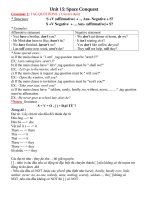
The mechanical counter is shown in Fig. 16.1.1. Motion of the event
being counted deflects the arm, which through an appropriate linkage
advances the count register one unit. Alternatively, motion of the actu-

Fig. 16.1.1

Mechanical counter.


Copyright (C) 1999 by The McGraw-Hill Companies, Inc. All rights reserved. Use of
this product is subject to the terms of its License Agreement. Click here to view.

MASS AND WEIGHT MEASUREMENT

ating arm may close an electrical switch which energizes a relay coil to

advance the count register one step.
Where there is a desire to avoid contact or close proximity with the
object being counted, the photoelectric cell or diode, in conjunction
with a lamp, a light-emitting diode (LED), or a laser light source, is
employed in the transmitted or reflected light mode (Fig. 16.1.2). A
signal to a counter is generated whenever the received light level is
altered by the passing objects. Objects may be very small and very high
counting speeds may be achieved with electronic counters.

Fig. 16.1.2 Photoelectric counter.

Sensing methods based on electrical capacitance, magnetic, and
eddy-current effects are extremely sensitive and fast acting, and are
suitable for objects in close proximity to the sensor. The capacitive probe senses dielectrics other than air, such as glass and plastic
parts. The magnetic pickup, by induction, responds to the motion of
iron and nickel. The eddy-current sensor, by energy absorption, detects
nonmagnetic conductors. All are suitable for counting machine operations.
The count is displayed by either a mechanical register as in Fig.
16.1.1, a dial-type register (as on the household watthour meter), or an
electronic pulse counter with either number indicators or digital printing
output. Electronic counters can operate accurately at rates exceeding 1
million counts per second.

TIME AND FREQUENCY MEASUREMENT

Measurement of time is basic to time and motion studies, time program
controls, and the measurements of velocity, frequency, and flow rate.
(See also Sec. 1.)
Mechanical clocks, chronometers, and stopwatches measure time in
terms of the natural oscillation period of a system such as a pendulum,

or hairspring balance-wheel combination. The minimum resolution is
one-half period. Since this period is somewhat affected by temperature,
precise timepieces employ a compensating element to maintain timing
accuracies over long periods. Stopwatches may be obtained to read to
better than 0.1 s. The major limitation, however, is in the response time
of the user.
Electric timers are simple, inexpensive, and readily adaptable to remote-control operations. The majority of these are ac synchronous
motors geared in the proper ratio to the indicator. These depend for their
accuracy on the frequency of the line voltage. Consequently, care must
be exercised in using such devices for precise short-time measurements.
Electronic timers are started and stopped by electrical pulses and
hence are not limited by the observer’s reaction time. They may be
made extremely accurate and capable of measuring to less than 1 ␮s.
These measure time by counting the number of cycles in a high-frequency signal generated internally by means of a quartz crystal. Stopwatch versions read at 0.01 s. Commercial instruments offer one or
more functions: counting, measurement of frequency, period, and time
intervals. Microprocessor-equipped versions increase versatility.
There are a variety of timing devices designed to indicate or control

16-3

to a fixed time. These include timers based on the charging time of a
condenser (e.g., type 555 integrated circuit), and the flow of oil or other
fluid through a restriction.
Timing devices can be calibrated by comparison with a standard instrument or by reference to the National Institute of Standards and
Technology timed radio signals, carrier frequencies and audio modulation of radio stations WWV and WWVB, Colorado, and WWVH,
Hawaii. WWV and WWVH broadcast with carrier frequencies of 2.5, 5,
10, and 15 MHz. WWV also broadcasts on 20 MHz. Broadcasts provide
second, minute, and hour marks with once-per-minute time announcements by voice and binary-coded decimal (BCD) signal on a 100-Hz
subcarrier. Standard audio frequencies of 440, 500, and 600 Hz are
provided. Station WWVB uses a 60-kHz carrier and provides second

and minute marks and BCD time and date. Time services are also issued
by NIST from geostationary satellites of the National Oceanographic
and Atmospheric Administration (NOAA) on frequencies of 468.8375
MHz for the 75° west satellite and 468.825 MHz for the 105° west
satellite. Automated Computer Time Service (ACTS) is available to
300- or 1200-baud modems via phone number 303-494-4774. (See also
Sec. 1.2.)
Fast-moving, repetitive motions may be timed and studied by the use
of stroboscopes which generate brilliant, very brief flashes of light at an
adjustable rate.
The frequency of the observed motion is measured by adjusting the
stroboscopic frequency until the system appears to stand still. The frequency of the motion is then equal to the stroboscope frequency or an
integer multiple of it.
Many other means exist for measuring vibrational or rotational frequencies. These include timing a fixed number of rotations or oscillations of the moving member. Contact sensing can be done by an attached switch, or noncontact sensing can be done by magnetic or optical
means. The pulses can be counted by an electronic counter or displayed
on an oscilloscope or recorder and compared with a known frequency.
Also used are reeds which vibrate when the measured oscillation excites
their natural frequencies, flyball devices which respond directly to angular velocity, and generator-type tachometers which generate a voltage
proportional to the speed.
MASS AND WEIGHT MEASUREMENT

Mass is the measure of the quantity of matter. The fundamental unit is
the kilogram. The U.S. customary unit is the pound; 1 lb ϭ 0.4536 kg
(see Sec. 1.2, ‘‘Measuring Units’’). Weight is a measure of the force of
gravity acting on a mass (see ‘‘Units of Force and Mass’’ in Sec. 4).
A general equation relating weight W and mass M is W/g ϭ M/gc ,
where g is the local acceleration of gravity, and gc ϭ 32.174 lbm и ft/
(lbf) (s2) [(1 kg и m/(N) (s2)] is a property of the unit system. Then W ϭ
Mg/gc . The specific weight w and the mass density p are related by w ϭ
pg/gc . Masses are conveniently compared by comparing their weights,

and masses are often loosely referred to as weights. Indeed, almost all
practical measures of mass are based on weight.
Weighing devices fall into two major categories: balances and forcedeflection systems. The device may be batch or continuous weighing,
automatic or manual. Accuracies are expected to be of the order of 0.1
to better than 0.0001 percent, depending on the type and application of
the scale. Calibration is normally performed by use of standard weights
(masses) with calibrations traceable to the National Institute of Standards and Technology.
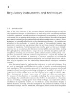
The equal arm balance compares the weight of an object with a set of
standard weights. The laboratory balance shown in Fig. 16.1.3 is used
for extreme precision and sensitivity. A chain poise provides fine adjustment of the final balance weight. The magnetic damper causes the
balance to come to equilibrium quickly.
Large weighing scales operate on the same principle; however, the
arms are unequal to allow multiplication between the tare and the measured weights. In this group are platform, track, hopper, and tank scales.
Here balance is achieved by adjusting the position of one or more balance weights along a beam directly calibrated in weight units. In dial-


Copyright (C) 1999 by The McGraw-Hill Companies, Inc. All rights reserved. Use of
this product is subject to the terms of its License Agreement. Click here to view.

16-4

INSTRUMENTS

indicating-type scales, balance is achieved automatically through the
deflection of calibrated pendulum weights from the vertical. The deflection is greatly magnified by the pointer-actuating mechanism, providing a direct-reading weight indication on the dial.

In continuous weighers, a section of conveyor belt is balanced on a
weigh beam (Fig. 16.1.5). The belt is driven at a constant speed; hence,
if the total weight is held constant, the weight rate of material fed
through the scale is fixed. Unbalance of the weight beam causes the rate

of material flow onto the belt to be changed in the direction of restoring
balance. This is accomplished by a mechanical adjustment of the feed
gate or by varying the speed of a belt or screw feeder drive.

Fig. 16.1.3 Laboratory balance.

Since the deflection of a spring (within its design range) is directly
proportional to the applied force, a calibrated spring serves as a simple
and inexpensive weighing device. Applications include the spring scale
and torsion balance. These are subject to hysteresis and temperature
errors and are not used for precise work.
Other force-sensing elements are adaptable to weight measurement.
Strain-gage load cells eliminate pivot maintenance and moving parts
and provide an electrical output which can be used for direct recording
and control purposes. Pneumatic pressure cells are also used with similar advantages.
In production processes, continuous and automatic operating scales are
employed. In one type, the balancing weight is positioned by a reversible electric motor. Deflection of the beam makes an electrical contact
which drives the motor in the proper direction to restore balance. The
final balance position is translated by means of a potentiometer or digital encoding disk into a signal which is used for recording or control
purposes.
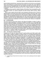
The batch-type scale (Fig. 16.1.4) is adaptable to continuous flow
streams of either liquids or solid particles. Material flows from the feed
hopper through an adjustable gate into the scale hopper. When the
weight in the scale hopper reaches that of the tare, the trip mechanism
operates, closing the gate and opening the door. As soon as the scale
hopper is empty, the weight of the tare forces the door closed again,
resets the trip, and opens the gate to repeat the cycle. The agitator rotates

Fig. 16.1.4 Automatic batch-weighing scale.


while the gate is open, to prevent the solids from packing. Also, a
‘‘dribble’’ (partial closing of the gate just before the mechanism trips) is
employed to minimize the error from the falling column of material at
the instant balance is achieved. Since each dump of the scale represents
a fixed weight, a counter yields the total weight of material passing
through the scale.

Fig. 16.1.5

Continuous-weighing scale.

If the density of the material is constant, volume measurements may be
used to determine the mass. Thus, calibrated tanks are frequently used
for liquids and vane and screw-type feeders for solids. Though often
simpler to apply, these are not generally capable of as high accuracies as
are common in weighing.

MEASUREMENT OF LINEAR AND ANGULAR
DISPLACEMENT
Displacement-measuring devices are employed to measure dimension,
distances between points, and some derived quantities such as velocity,
area, etc. These devices fall into two major categories: those based on
comparison with a known or reference length and those based on some
fixed physical relationship.
The measurement of angles is closely related to displacement measurements, and indeed, one is often converted into the other in the process of
measurement. The common unit is the degree, which represents 1⁄360 of
an entire rotation. The radian is used in mathematics and is related to the
degree by ␲ rad ϭ 180°; 1 rad ϭ 57.3°. The grad is an angle unit ϭ 1⁄400
rotation.
Figure 16.1.6 illustrates some methods of rotary to linear conversion.

Figure 16.1.6a is a simple link and lever, Fig. 16.1.6b is a flexible link
and sector, and Fig. 16.1.6c is a rack-and-pinion mechanism. These can
be used to convert in either direction according to the relationship D ϭ
RA/57.3, where R ϭ mean radius of the rotating element, in; D ϭ
displacement, in; and A ϭ rotation, deg. (This equation holds for the
link and lever of Fig. 16.1.6a only if the angle change from the perpendicular is small.)
Comparative devices are generally of the indicating type and include
ruled or graduated devices such as the machinist’s scale, folding rule,
tape measure, digital caliper (Fig. 16.1.7), digital micrometer (Fig.
16.1.8), etc. These vary widely in their accuracy, resolution, and measuring span, according to their intended application. The manual readings depend for their accuracy on the skill and care of the operator.
The digital caliper and digital micrometer provide increased sensitivity and precision of reading. The stem of the digital caliper carries an
embedded encoded distance scale. That scale is read by the slider. The
distance so found shows on the digital display. The device is batteryoperated and capable of displaying in inches or millimeters. Typical
resolution is 0.0005 in or 0.01 mm.
The digital micrometer, employing rotation and translation to stretch
the effective encoded scale length, provides resolution to 0.0001 in or
0.003 mm.


Copyright (C) 1999 by The McGraw-Hill Companies, Inc. All rights reserved. Use of
this product is subject to the terms of its License Agreement. Click here to view.

MEASUREMENT OF LINEAR AND ANGULAR DISPLACEMENT

16-5

Fig. 16.1.6 Linear-rotary conversion mechanisms.

D
(external)


Mode marker
Measured value, D (or d)
mm
I

1.035
I/O

mm/I

zero

Embedded
distance encoder
d
(internal)

ON/OFF
zero

mm or inch
display

Displacement can be measured electrically through its effect on the
resistance, inductance, reluctance, or capacitance of an appropriate
sensing element.
The potentiometer is comparatively inexpensive, accurate, and flexible in application. It consists of a fixed linear resistance over which
slides a rotating contact keyed to the input shaft (Fig. 16.1.9). The
resistance or voltage (assuming constant voltage across terminals 1 and

3) measured across terminals 1 and 2 is directly proportional to the
angle A. For straight-line motion, a mechanism of the type shown in Fig.
16.1.6 converts to rotary motion (or a rectilinear-type potentiometer can
be used directly). (See also Sec. 15.) Versions with multiturns, straightline motion, and special nonlinear resistance vs. motion are available.

Fig. 16.1.7 Digital caliper.
Dial gages are also used to magnify motion. A rack and pinion (Fig.
16.1.6c) converts linear into rotary motion, and a pointer moves over a
calibrated scale.
Various modifications of the above-mentioned devices are available
for making special kinds of measurements; e.g., depth gages for measuring the depth of a hole or cavity, inside and outside calipers (Fig. 16.1.7)
for measuring the internal and external dimensions respectively of an
object, protractors for angular measurement, etc.

Embedded sleeve
and distance encoder

Fig. 16.1.9

Thimble

Spindle
D
.

.

.

.


.

.

.

mm
I

.

.

.

0.2736

On/Off

mm/I

Zero

Fig. 16.1.8 Digital micrometer.

For line production and inspection work, go no-go gages provide a
rapid and accurate means of dimension measurement and control. Since
the measured values are fixed, the dependence on the operator’s skill is
considerably reduced. Such gages can be very complex in form to embrace a multidimensional object. They can also take the more general

forms of the feeler, wire, or thread-gage sets. Of particular importance are
precision gage blocks, which are used as standards for calibrating other
measuring devices.

Potentiometer.

The synchro, the linear variable differential transformer (LVDT), and
the E transformer are devices in which the input motion changes the
inductive coupling between primary and secondary coils. These avoid
the limitations of wear, friction, and resolution of the potentiometer, but
they require an ac supply and usually an electronic amplifier for the
output. (See also Sec. 15.)
The synchro is a rotating device which is used to transmit rotary
motions to a remote location for indication or control action. It is particularly useful where the rotation is continuous or covers a wide range.
They are used in pairs, one transmitter and one receiver. For measurement of difference in angular position, the control-transmitter and control-transformer synchros generate an electrical error signal useful in
control systems. A synchro differential added to the pair serves the same
purpose as a gear differential.
The linear variable differential transformer (LVDT) consists of a primary and two secondary coils wound around a common core (Fig.
16.1.10). An armature (iron) is free to move vertically along the axis of
the coils. An ac voltage is applied to the primary. A voltage is induced in
each secondary coil proportional to the relative length of armature linking it with the primary. The secondaries are connected to oppose each
other so that when the armature is centered, the output voltage is zero.


Copyright (C) 1999 by The McGraw-Hill Companies, Inc. All rights reserved. Use of
this product is subject to the terms of its License Agreement. Click here to view.

16-6

INSTRUMENTS


When the armature is displaced off center by an amount D, the output
will be proportional to D (and phased to show whether D is above or
below the center). These devices are very linear near the centered position, require negligible actuating force, and have spans ranging from 0.1
to several inches (0.25 cm to several centimeters).

Fig. 16.1.10 Linear variable differential transformer (LVDT).

The E transformer is very similar to the above except that the coils are
wound around a laminated iron core in the shape of an E (with the
primary and secondaries occupying the center and outside legs respectively). The magnetic path is completed through an armature whose
motion, either rotary or translational, varies the induced voltage in the
secondaries, as in the device of Fig. 16.1.10. This, too, is sensitive to
extremely small motions.
A method that is readily applied, if a strain-gage analyzer is handy, is
to measure the deflection of a cantilever spring with strain gages bonded
to its surface (see Strain Gages, Sec. 5).
The change of capacitance with the displacement of the capacitor
plates is extremely sensitive and suitable to very small displacements or
large rotation. Often, one plate is fixed within the instrument; the other
is formed or rotated by the object being measured. The capacitance can
be measured by an impedance bridge, by determining the resonant frequency of a tuned circuit or using a relaxation oscillator.
Many optical instruments are available for obtaining precise measurements. The transit and level are used in surveying for measuring
angles and vertical distances (see Sec. 16.3). A telescope with fine cross
hairs permits accurate sighting. The angle scales are generally equipped
with verniers. The measuring microscope permits measurement of very
small displacements and dimensions. The microscope table is equipped
with micrometer screws for sensitive adjustment. In addition, templates
of scales, angles, etc., are available to permit measurement by comparison. The optical comparator projects a magnified shadow image of an
object on a screen where it can readily be compared with a reference

template.
Light can be used as a standard for the measurement of distance,
straightness, and related properties. The wavelength of light in a medium is the velocity of light in vacuum divided by the index of refraction n of the medium. For dry air n Ϫ 1 is closely proportional to air
density and is about 0.000277 at 1 atm and 15°C for 550-nm green light.
Since the wavelength changes about ϩ 1 ppm/°C, and about Ϫ 0.36
ppm/mmHg, density gradients bend light slightly. A temperature gradient of 1°C/m (0.5°F/ft) will cause a deviation from a tangent line of
about 0.05 mm (0.002 in) at 10 m (33 ft).
Optical equipment to establish and test alignment, plumb lines,
squareness, and flatness includes jig transits, alignment telescopes, collimators, optical squares, mirrors, targets, and scales.
Interference principles can be used for distance measurements. An
optical flat placed in close contact with a polished surface and illuminated perpendicular to the surface with a monochromatic light will
show interference bands which are contours of constant separation distance between the surfaces. Adjacent bands correspond to separation
differences of one-half wavelength. For 550-nm wavelength this is
275 nm (10.8 ␮in). This test is useful in examining surfaces for flatness
and in length comparisons with gage blocks.

Laser beams can be used over great distances. Surveying instruments
are available for measurements up to 40 mi (60 km). Accuracy is stated
to be about 5 mm (0.02 ft) ϩ 1 ppm. These instruments take several
measurements which are processed automatically to display the distance directly. Momentary interruptions of the light beam can be tolerated.
A laser system for machine tools, measurement tables, and the like is
available in modular form (Hewlett-Packard Co.). It can serve up to
eight axes by using beam splitters with a combined range of 200 ft
(60 m). Normal resolution of length is about one-fourth wavelength,
with a digital display least count of 10 ␮in (0.1 ␮m). Angle-measurement display resolves 0.1 second of arc. Accuracy with proper environmental compensation is stated to be better than 1 ppm ϩ 1 count in
length measurement. Velocities up to 720 in/min (0.3 m/s) can be followed. Accessories are available for measuring straightness, parallelism, squareness and flatness, and for automatic temperature compensation. Various output options include displays and automatic
computation and plots. The system can be used directly in measurement
and control or to calibrate lead screws and other conventional measuring devices.
Pneumatic gaging finds an important place in line inspection and quality control. The device (Fig. 16.1.11) consists of a nozzle fixed in position relative to a stop or jig. Air at constant supply pressure passes
through a restriction and discharges through the nozzle. The nozzle

back pressure P depends on the gap G between the measured surface
and the nozzle opening. If the measured dimension D increases, then G
decreases, restricting the discharge of air, increasing P. Conversely,
when D decreases, P decreases. Thus, the pressure gage indicates deviation of the dimension from some normal value. With proper design,

Fig. 16.1.11

Pneumatic gage.

this pressure is directly proportional to the deviation, limited, however,
to a few thousandths of an inch span. The device is extremely sensitive
[better than 0.0001 in (0.003 mm)], rugged, and, with periodic calibration against a standard, quite accurate. The gage is adaptable to automatic line operation where the pressure signal is recorded or used to
actuate ‘‘reject’’ or ‘‘accept’’ controls. Further, any number of nozzles
can be used in a jig to check a multiplicity of dimensions. In another
form of this device, the flow of air is measured with a rotameter in place
of the back pressure. The linear-variable differential transformer
(LVDT) is also applicable.
The advent of automatically controlled machine tools has brought
about the need for very accurate displacement measurement over a wide

Fig. 16.1.12

Radiation-type thickness gage.


Copyright (C) 1999 by The McGraw-Hill Companies, Inc. All rights reserved. Use of
this product is subject to the terms of its License Agreement. Click here to view.

FORCE AND TORQUE MEASUREMENT


range. Most commonly applied for this purpose is the calibrated lead
screw which measures linear displacement in terms of its angular rotation. Digital systems greatly extend the resolution and accuracy limitations of the lead screw. In these, a uniformly spaced optical or inductive
grid is displaced relative to a sensing element. The number of grid lines
counted is a direct measure of the displacement (see discussion of lasers
above).
Measurement of strip thickness or coating thickness is achieved by
X-ray or beta-radiation- type gages (Fig. 16.1.12). A constant radiation
source (X-ray tube or radioisotope) provides an incident intensity I0; the
radiation intensity I after passing through the absorbing material is
measured by an appropriate device (scintillation counter, Geiger-M¨uller
tube, etc.). The thickness t is determined by the equation I ϭ I0eϪ kt,
where k is a constant dependent on the material and the measuring
device. The major advantage here is that measurements are continuous
and nondestructive and require no contact. The method is extended to
measure liquid level and density.
MEASUREMENT OF AREA

Area measurements are made for the purpose of determining surface
area of an object or area inside a closed curve relating to some desired
physical quantity. Dimensions are expressed as a length squared; e.g.,
in2 or m2. The areas of simple forms are readily obtained by formula.
The area of a complex form can be determined by subdividing into
simple forms of known area. In addition, various numerical methods are
available (see Simpson’s rule, Sec. 2) for estimating the area under irregular curves.
Area measuring devices include various mechanical, electrical, or
electronic flow integrators (used with flowmeters) and the polar planimeter. The latter consists of two arms pivoted to each other. A tracer at the
end of one arm is guided around the boundary curve of the area, causing
rotation of a recorder wheel proportional to the area enclosed.
MEASUREMENT OF FLUID VOLUME


For a liquid of known density, volume is a quick and simple means of
measuring the amount (or mass) of liquid present. Conversely, measuring the weight and volume of a given quantity of material permits
calculation of its density. Volume has the dimensions of length cubed;
e.g., cubic metres, cubic feet. The volume of simple forms can be obtained by formula.
A volumetric device is any container which has a known and fixed
calibration of volume contained vs. the level of liquid. The device may
be calibrated at only one point (pipette, volumetric flask) or may be graduated over its entire volume (burette, graduated cylinder, volumetric tank).
In the case of the tank, a sight glass may be calibrated directly in liquid
volume.
Volumetric measure of continuous flow streams is obtained with the
displacement meter. This is available in various forms: the nutating disk,
reciprocating piston, rotating vane, etc. The nutating-disk meter (Fig.
16.1.13) is relatively inexpensive and hence is widely used (water
meters, etc.). Liquid entering the meter causes the disk to nutate or
‘‘roll’’ as the liquid makes its way around the chamber to the outlet. A
pin on the disk causes a counter to rotate, thereby counting the total
number of rolls of the disk. Meter accuracy is limited by leakage past
the disk and friction. The piston meter is like a piston pump operated

backward. It is used for more precise measure (available to 0.1 percent
accuracy).
Volumetric gas measurement is commonly made with a bellows
meter. Two bellows are alternately filled and exhausted with the gas.
Motion of the bellows actuates a register to indicate the total flow.
Various liquid-sealed displacement meters are also available for this
purpose.
For precise volume measurements, corrections for temperature must
be made (because of expansion of both the material being measured and
the volumetric device). In the case of gases, the pressure also must be
noted.

FORCE AND TORQUE MEASUREMENT
Force may be measured by the deflection of an elastic element, by
balancing against a known force, by the acceleration produced in an
object of known mass, or by its effects on the electrical or other properties of a stress-sensitive material. The common unit of force is the
pound (newton). Torque is the product of a force and the perpendicular
distance to the axis of rotation. Thus, torque tends to produce rotational
motion and is expressed in units of pound feet (newton metres). Torque
can be measured by the angular deflection of an elastic element
or, where the moment arm is known, by any of the force measuring
methods.
Since weight is the force of gravity acting on a mass, any of the
weight-measuring devices already discussed can be used to measure
force. Common methods employ the deflection of springs or cantilever
beams.
The strain gage is an element whose electrical resistance changes
with applied strain (see Sec. 5). Combined with an element of known
force-strain, motion-strain, or other input-strain relationship it is a
transducer for the corresponding input. The relation of gage-resistance
change to input variable can be found by analysis and calibration. Measure of the resistance change can be translated into a measure of the
force applied. The gage may be bonded or unbonded. In the bonded
case, the gage is cemented to the surface of an elastic member and
measures the strain of the member. Since the gage is very sensitive to
temperature, the readings must be compensated. For this purpose, four
gages are connected in a Wheatstone-bridge circuit such that the temperature effect cancels itself. A four-element unbonded gage is shown
in Fig. 16.1.14. Note that as the applied force increases, the tension on
two of the elements increases while that on the other two decreases.
Gages subject to strain change of the same sign are put in opposite arms
of the bridge. The zero adjustment permits balancing the bridge for zero
output at any desired input. The e1 and e2 terminal pairs may be used
interchangeably for the input excitation and the signal output.


Fig. 16.1.14

Fig. 16.1.13 Nutating-disk meter.

16-7

Unbonded strain-gage board.

The piezoelectric effect is useful in measuring rapidly varying forces
because of its high-frequency response and negligible displacement
characteristics. Quartz rochelle salt, and barium titanate are common
piezoelectric materials. They have the property of varying an output
charge in direct proportion to the stress applied. This produces a voltage
inversely proportional to the circuit capacitance. Charge leakage produces drifting at a rate depending on the circuit time constant. The


Copyright (C) 1999 by The McGraw-Hill Companies, Inc. All rights reserved. Use of
this product is subject to the terms of its License Agreement. Click here to view.

16-8

INSTRUMENTS

voltage must be measured with a device having a very high input resistance. Accuracy is limited because of temperature dependence and
some hysteresis effect.
Forces may also be measured with any of the pressure devices described in the next section by balancing against a fluid pressure acting
on a fixed area.
PRESSURE AND VACUUM MEASUREMENT


Pressure is defined as the force per unit area exerted by a fluid. Pressure
devices normally measure with respect to atmospheric pressure (mean
value ϭ 14.7 lb/in2), pa ϭ pg ϩ 14.7, where pa ϭ total or absolute
pressure and pg ϭ gage pressure, both lb/in2. Conventionally, gage pressure and vacuum refer to pressures above and below atmospheric, respectively. Common units are lb/in2, in Hg, ftH2O, kg/cm2, bars, and
mmHg. The mean SI atmosphere is 1.013 bar.
Pressure devices are based on (1) measure of an equivalent height of
liquid column; (2) measure of the force exerted on a fixed area; (3)
measure of some change in electrical or physical characteristics of the
fluid.
The manometer measures pressure according to the relationship p ϭ
wh ϭ ␳gh/gc , where h ϭ height of liquid of density ␳ and specific
weight w (assumed constants) supported by a pressure p. Thus, pressures are often expressed directly in terms of the equivalent height
(head) of manometer liquid, e.g., inH 2O or inHg. Usual manometer
fluids are water or mercury, although other fluids are available for special ranges.
The U-tube manometer (Fig. 16.1.15a) expresses the pressure difference p1 Ϫ p2 as the difference in levels h. If p2 is exposed to the
atmosphere, the manometer reads the gage pressure of p1 . If the p2 tube
is evacuated and sealed ( p2 ϭ 0), the absolute value of p1 is indicated. A
common modification is the well-type manometer (Fig. 16.1.15b). The
scale is specially calibrated to take into account changes of level inside
the well so that only a single tube reading is required. In particular, Fig.
16.1.15b illustrates the form usually applied to measurement of atmospheric pressure (mercury barometer).

commonly, the unknown pressure is balanced against an air or hydraulic
pressure, which in turn is measured with a gage. By use of unequal-area
diaphragms, the pressure can thus be amplified or attenuated as required. Further, it permits isolating the process fluid which may be
corrosive, viscous, etc.
The Bourdon-tube gage (Fig. 16.1.16) is the most commonly used
pressure device. It consists of a flattened tube of spring bronze or steel
bent into a circle. Pressure inside the tube tends to straighten it. Since
one end of the tube is fixed to the pressure inlet, the other end moves

proportionally to the pressure difference existing between the inside and
outside of the tube. The motion rotates the pointer through a pinionand-sector mechanism. For amplification of the motion, the tube may be
bent through several turns to form spiral or helical elements as are used
in pressure recorders.

Fig. 16.1.16

Bourdon-tube gage.

In the diaphragm gage, the pressure acts on a diaphragm in opposition
to a spring or other elastic member. The deflection of the diaphragm is
therefore proportional to the pressure. Since the force increases with the
area of the diaphragm, very small pressures can be measured by the use
of large diaphragms. The diaphragm may be metallic (brass, stainless
steel) for strength and corrosion resistance, or nonmetallic (leather,
neoprene, silicon, rubber) for high sensitivity and large deflection. With
a stiff diaphragm, the total motion must be very small to maintain linearity.
The bellows gage (Fig. 16.1.17) is somewhat similar to the diaphragm
gage, with the advantage, however, of providing a much wider range of
motion. The force acting on the bottom of the bellows is balanced by the
deflection of the spring. This motion is transmitted to the output arm,
which then actuates a pointer or recorder pen.

Fig. 16.1.15 Manometers. (a) U tube; (b) well type.

The sensitivity of readings can be increased by inclining the manometer tubes to the vertical (inclined manometer), by use of low-specificgravity manometer fluids, or by application of optical-magnification or
level-sensing devices. Accuracy is influenced by surface-tension effects
(reading of the meniscus) and changes in fluid density (due to temperature changes and impurities).
By definition, pressure times the area acted upon equals the force
exerted. The pressure may act on a diaphragm, bellows, or other element of fixed area. The force is then measured with any force-measuring device, e.g., spring deflection, strain gage, or weight balance. Very


Fig. 16.1.17

Bellows gage.


Copyright (C) 1999 by The McGraw-Hill Companies, Inc. All rights reserved. Use of
this product is subject to the terms of its License Agreement. Click here to view.

TEMPERATURE MEASUREMENT

The motion (or force) of the pressure element can be converted into
an electrical signal by use of a differential transformer or strain-gage
element or into an air-pressure signal through the action of a nozzle and
pilot. The signal is then used for transmission, recording, or control.
The dead-weight tester is used as a standard for calibrating gages.
Known hydraulic or gas pressures are generated by means of weights
loaded on a calibrated piston. The useful range is from 5 to 5,000 lb/in2
(0.3 to 350 bar). For low pressures, the water or mercury manometer
serves as a reference.
For many applications (fluid flow, liquid level), it is important to
measure the difference between two pressures. This can be done directly
with the manometer. Other pressure devices are available as differential
devices where (1) the case is made pressure-tight so that the second
pressure can be applied external to the pressure element; (2) two identical pressure elements are mounted so that their outputs oppose each
other.
Similar devices to those discussed are used to measure vacuum, the
only difference being a shift in range or at most a relocation of the
zeroing spring. When the vacuum is high (absolute pressure near zero)
variations in atmospheric pressure become an important source of error.

It is here that absolute-pressure devices are employed.
Any of the differential-pressure elements can be converted to an absolute-pressure device by sealing one pressure side to a perfect vacuum.
A common instrument for the range 0 to 30 inHg employs two bellows
of equal area set back to back. One bellows is completely evacuated and
sealed; the other is connected to the measured pressure. The output is a
bellows displacement, as in Fig. 16.1.17.
There are many instruments for high-vacuum work (0.001 to
10,000 ␮m range). These kinds of devices are based on the characteristic properties of gases at low pressures. The McLeod gage amplifies the
pressure to be measured by compressing the gas a known amount and
then measuring its pressure with a mercury manometer. The ratio of
initial to final pressure is equal to the ratio of final to initial volume (for
common gases). This gage serves as a standard for low pressures.
The Pirani gage (Fig. 16.1.18) is based on the change of heat conductivity of a gas with pressure and the change of electrical resistance of a
wire with temperature. The wire is electrically heated with a constant
current. Its temperature changes with pressure, producing a voltage
across the bridge network. The compensating cell corrects for roomtemperature changes.

Fig. 16.1.18 Pirani gage.

The thermocouple gage is similar to the Pirani gage, except that a
thermocouple is used to measure the temperature difference between the
resistance elements in the measuring and compensating cells, respectively.
The ionization gage measures the ion current generated by bombardment of the molecules of the gas by the electron stream in a triode-type
tube. This gage is limited to pressures below 1 ␮m. It is, however,
extremely sensitive.
LIQUID-LEVEL MEASUREMENT

Level instruments are used for determining (or controlling) the height of
liquid in a vessel or the location of the interface between two liquids of
different specific gravity. In large storage tanks the level is indicated by

a calibrated tape or chain which is attached to a float riding the liquid

16-9

surface or by converting the signal reflection time of a radar or ultrasonic beam radiated onto the surface of the liquid into a level indication.
For measuring small changes in level, the fixed displacer is common
(Fig. 16.1.19). The buoyant force is proportional to the volume of displacer submerged and hence changes directly with the level. The force
is balanced by the air pressure acting in the bellows, which in turn is
generated by the flapper and nozzle. A pressure gage (or recorder)
indicates the level.

Fig. 16.1.19

Displacer-type level meter.

The level is often measured by means of a differential-pressure meter
connected to taps in the top and bottom of the tank. As indicated in the
discussion on manometers, the pressure difference is the height times
the specific weight of the liquid. Where the liquid is corrosive or contains solids, then liquid seals, water purge, or air purge may be used to
isolate the meter from the process.
For special applications, the dielectric, conducting, or absorption
properties of the liquid can be used. Thus, in one model the liquid rises
between two plates of a condenser, producing a capacitance change proportional to the change in level, and in another the radiation from a small
radioactive source is measured. Since the liquid has a high absorption
for the rays (compared with the vapor space), the intensity of the measured radiation decreases with the increase in level. An important advantage of this type is that it requires no external connections to the
process.
TEMPERATURE MEASUREMENT

The common temperature scales (Fahrenheit and Celsius) are based on
the freezing and boiling points of water (see Sec. 4 for discussion of

temperature standards, units, and conversion equations).
Temperature is measured in a number of different ways. Some of the
more useful are as follows.
1. Thermal expansion of a gas (gas thermometer). At constant volume, the pressure p of an (ideal) gas is directly proportional to its
absolute temperature T. Thus, p ϭ (p0 /T0)T, where p0 is the pressure at
some known temperature T0 .
2. Thermal expansion of a liquid or solid (mercury thermometer, bimetallic element). Substances tend to expand with temperature. Thus, a
change in temperature t2 Ϫ t1 causes a change in length l2 Ϫ l1 or a
change in volume V2 Ϫ V1 , according to the expressions.
l2 Ϫ l1 ϭ aЈ(t2 Ϫ t1)l1

or V2 Ϫ V1 ϭ aЈЈЈ(t2 Ϫ t1)V1

where aЈ and aЈЈЈ ϭ linear and volumetric coefficients of thermal expansion, respectively (see Sec. 4). For many substances, aЈ and aЈЈЈ
are reasonably constant over a limited temperature range. For solids,
aЈЈЈ ϭ 3aЈ. For mercury at room temperature, aЈЈЈ is approximately
0.00018°CϪ 1 (0.00010°FϪ 1).
3. Vapor pressure of a liquid (vapor-bulb thermometer). The vapor
pressure of all liquids increases with temperature. The Clapeyron equation permits calculation of the rate of change of vapor pressure with
temperature.
4. Thermoelectric potential (thermocouple). When two dissimilar
metals are brought into intimate contact, a voltage is developed which
depends on the temperature of the junction and the particular metals


Copyright (C) 1999 by The McGraw-Hill Companies, Inc. All rights reserved. Use of
this product is subject to the terms of its License Agreement. Click here to view.

16-10


INSTRUMENTS

used. If two such junctions are connected in series with a voltage-measuring device, the measured voltage will be very nearly proportional to
the temperature difference of the two junctions.
5. Variation of electrical resistance (resistance thermometer, thermistor). Electrical conductors experience a change in resistance with temperature which can be measured with a Wheatstone- or Mueller-bridge
circuit, or a digital ohmmeter. The platinum resistance thermometer
(PRT) can be very stable and is used as the temperature scale interpolation standard from Ϫ 160 to 660°C. Commercial resistance temperature
detectors (RTD) using copper, nickel, and platinum conductors are in
use and are characterized by a polynomial resistance-temperature relationship, such as
t ϭ A ϩ B ϫ Rt ϩ C ϫ R2t ϩ D ϫ R3t ϩ E ϫ R4t
where Rt ϭ resistance at prevailing temperature t in °C. A, B, C, D, and
E are range- and material-dependent coefficients listed in Table 16.1.1.
R0 , also shown in the table, is the base resistance at 0°C used in the
identification of the sensor.
The thermistor has a large, negative temperature coefficient of resistance, typically Ϫ 3 to Ϫ 6 percent/°C, decreasing as temperature increases. The temperature-resistance relation is approximated (to perhaps 0.01° in range 0 to 100°C) by:
Rt ϭ exp
and

ͩ

A0 ϩ A1 /t ϩ

A2
A
ϩ 33
t2
t

ͪ


␭m ϭ k1/T

l
ϭ a0 ϩ a1 ln Rt ϩ a2(ln Rt)2 ϩ a3(ln Rt)3
t

with the constants chosen to fit four calibration points. Often a simpler
form is given:
R ϭ R0 exp

ͭ ͫͩ ͪ ͩ ͪͬͮ
␤

l
t

Ϫ

l
t0

Typically
.
␤ varies in the range of 3,000 to 5,000 K. The reference
temperature t0 is usually 298 K(ϭ 25°C, 77°F), and R0 is the resistance
at that temperature. The error may be as small as 0.3°C in the range of 0°
to 50°C. Thermistors are available in many forms and sizes for use from
Ϫ 196 to ϩ 450°C with various tolerances on interchangeability and
matching. (See ‘‘Catalog of Thermistors,’’ Thermometrics, Inc.) The
AD590 and AD592 integrated circuit (Analog Devices, Inc.) passes a

current of 1 ␮A/°K very nearly proportional to absolute temperature.
All these sensors are subject to self-heating error.
6. Change in radiation (radiation and optical pyrometers). A body radiates energy proportional to the fourth power of its absolute temperature. This principle is particularly adaptable to the measurement of very
high temperatures where either the total quantity of radiation or its
intensity within a narrow wavelength band may be measured. In the
former type (radiation pyrometer), the radiation is focused on a heatsensitive element, e.g., a thermocouple, and its rise in temperature is
measured. In the latter type (optical pyrometer) the intensity of the
radiation is compared optically with a heated filament. Either the filament brightness is varied by a control calibrated in temperature, or a
fixed brightness filament is compared with the source viewed through a
calibrated optical wedge.
Table 16.1.1
Material
of
conductor

The infrared thermometer accepts radiation from an object seen in a
definite field of view, filters it to select a portion of the infrared spectrum, and focuses it on a sensor such as a blackened thermistor flake,
which warms and changes resistance. Electronic amplification and signal processing produce a digital display of temperature. Correct calibration requires consideration of source emissivity, reflection, and transmission from other radiation sources, atmospheric absorption between
the source object and the sensor, and compensation for temperature
variation at the sensor’s immediate surroundings.
Electrical nonconductors generally have fairly high (about 0.95)
emissivities, while good conductors (especially smooth, reflective metal
surfaces), do not; special calibration or surface conditioning is then
needed. Very wide band (0.7 to 20 ␮m) instruments gather relatively
large amounts of energy but include atmospheric absorption bands
which reduce the energy received from a distance. The band 8 to 14 ␮m
is substantially free from atmospheric absorption and is popular for
general use with source objects in the range 32 to 1,000°F (0 to 540°C).
Other bands and two-color instruments are used in some cases. See
Bonkowski, Infrared Thermometry, Measurements and Control, Feb.

1984, pp. 152 – 162.
Fiber-optics probes extend the use of radiation methods to hard-toreach places.
Important relationships used in the design of these instruments are the
Wien and Stefan-Boltzmann laws (in modified form):
q ϭ k2␧A(T 42 Ϫ T 41)

where ␭m ϭ wavelength of maximum intensity, ␮m (nm); q ϭ radiant
energy flux, Btu/h (W); A ϭ radiation surface, ft2 (m2); ␧ ϭ mean
emissivity of the surfaces; T2 , T1 ϭ absolute temperatures of radiating
and receiving surfaces, respectively, °R (K); k1 ϭ 5215 ␮m. °R (2898
␮m и K); k2 ϭ 0.173 ϫ 10Ϫ 8 Btu/(h и ft2 и °R4) [5.73 ϫ 10Ϫ 8
W/(m2 и K4)]. The emissivity depends on the material and form of the
surfaces involved (see Sec. 4). Radiation sensors with scanning capability can produce maps, photographs, and television displays showing
temperature-distribution patterns. They can operate with resolutions to
under 1°C and at temperatures below room temperature.
7. Change in physical or chemical state (Seger cones, Tempilsticks).
The temperatures at which substances melt or initiate chemical reaction
are often known and reproducible characteristics. Commercial products
are available which cover the temperature range from about 120 to
3600°F (50 to 2000°C) in intervals ranging from 3 to 70°F (2 to 40°C).
The temperature-sensing element may be used as a solid which softens
and changes shape at the critical temperature, or it may be applied as a
paint, crayon, or stick-on label which changes color or surface appearance. For most the change is permanent; for some it is reversible. Liquid
crystals are available in sheet and liquid form: these change reversibly
through a range of colors over a relatively narrow temperature range.
They are suitable for showing surface-temperature patterns in the range
20 to 50°C (68 to 122°F).
An often used temperature device is the mercury-in-glass thermometer.
As the temperature increases, the mercury in the bulb expands and rises
through a fine capillary in the graduated thermometer stem. Useful

range extends from Ϫ 30 to 900°F (Ϫ 35 to 500°C). In many applications of the mercury thermometer, the stem is not exposed to the mea-

Polynomial Coefficients for Resistance Temperature Detectors

ID R 0 , ⍀

Polynomial coefficients

Useful
range,
°C

A,
°C

B,
°C/⍀

C,
°C/⍀ 2

D,
°C/⍀ 3

Ϫ 70 to 0
0 to 150

Ϫ 225.64
Ϫ 234.69


23.30735
25.95508

ϩ 0.246864

Ϫ 0.00715

Copper
10⍀ @25°C

9.042

Nickel

120

Ϫ 80 to 320

Ϫ 199.47

1.955336

Ϫ 0.00266

1.88E Ϫ 6

100

Ϫ 200 to 0
0 to 850


Ϫ 241.86
Ϫ 236.06

2.213927
2.215142

0.002867
0.001455

Ϫ 9.8E Ϫ 6

Platinum
DIN/IEC
␣ ϭ 0.00385/°C

E,
°C/⍀ 4

Typical
accuracy,*
°C
1.5
1.5
1

1.64E Ϫ 8

* For higher accuracy consult the table or equation furnished by the manufacturer of the specific RTD being used. Temperatures per ITS-90, resistances per SI-90.


1
0.5


Copyright (C) 1999 by The McGraw-Hill Companies, Inc. All rights reserved. Use of
this product is subject to the terms of its License Agreement. Click here to view.

TEMPERATURE MEASUREMENT

sured temperature; hence a correction is required (except where the
thermometer has been calibrated for partial immersion). Recommended
formula for the correction K to be added to the thermometer reading is
K ϭ 0.00009 D(t1 Ϫ t2), where D ϭ number of degrees of exposed
mercury filament, °F; t1 ϭ thermometer reading, °F; t2 ϭ the temperature at about middle of the exposed portion of stem, °F. For Celsius
thermometers the constant 0.00009 becomes 0.00016.
For industrial applications the thermometer or other sensor is encased
in a metal or ceramic protective well and case (Fig. 16.1.20). A threaded
union fitting is provided so that the thermometer can be installed in a
line or vessel under pressure. Ideally the sensor should have the same
temperature as the fluid into which the well is inserted. However, heat

A common bimetallic pair consists of invar (iron-nickel alloy) and
brass.
For control or alarm indications at fixed temperatures, thermometers
may be equipped with electrical contacts such that when the temperature matches the contact point, an external relay circuit is energized.
A popular industrial-type instrument employs the deflection of a
pressure-spring to indicate (or record) the temperature (Fig. 16.1.22).
The sensing element is a metal bulb containing some specific gas or
liquid. The bulb connects with the pressure spring (in the form of a
spiral or helix) through a capillary tube which is usually enclosed in a


Fig. 16.1.22

Fig. 16.1.20 Industrial thermometer.

conduction to or from the pipe or vessel wall and radiation heat transfer
may also influence the sensor temperature (see ASME PTC 19.3-1974
Temperature Measurement, on well design). An approximation of the
conduction error effect is
Tsensor Ϫ Tfluid ϭ (Twall Ϫ Tfluid)E
For a sensor inserted to a distance L Ϫ x from the tip of a well of
insertion length L, E ϭ cosh[m(L Ϫ x)]/cosh mL, where m ϭ (h/kt)0.5; x
and L are in ft (m); h ϭ fluid-to-well conductance, Btu/(h) (ft2)(°F)
[J/(h) (m2)(°C)]; k ϭ thermal conductivity of the well-wall material.
Btu/(h)(ft)(°F) [J/(h)(m)(°C)]; and t ϭ well-wall thickness, ft (m). Good
thermal contact between the sensor and the well wall is assumed. For
(L Ϫ x)/L ϭ 0.25:
mL
E

1
0.67

2
0.30

3
0.13

4

0.057

5
0.025

6
0.012

7
0.005

Radiation effects can be reduced by a polished, low-emissivity surface
on the well and by radiation shields around the well. Concern with
mercury contamination has made the bimetal thermometer the most
commonly used expansion-based temperature measuring device. Differential thermal expansion of a solid is employed in the simple bimetal
(used in thermostats) and the bimetallic helix (Fig. 16.1.21). The bimetallic element is made by welding together two strips of metal having
different coefficients of expansion. A change in temperature then causes
the element to bend or twist an amount proportional to the temperature.

Fig. 16.1.21 Bimetallic temperature gage.

16-11

Pressure-spring element.

protective sheath or armor. Increasing temperature causes the fluid in
the bulb to expand in volume or increase in pressure. This forces the
pressure spring to unwind and move the pen or pointer an appropriate
distance upscale.
The bulb fluid may be mercury (mercury system), nitrogen under

pressure (gas system), or a volatile liquid (vapor-pressure system).
Mercury and gas systems have linear scales; however, they must be
compensated to avoid ambient temperature errors. The capillary may
range up to 200 ft in length with, however, considerable reduction in
speed of response.
For transmitting temperature readings over any distance (up to
1,000 ft), the pneumatic transmitter (Fig. 16.1.23) is better suited than
the methods outlined thus far. This instrument has the additional advantages of greater compactness, higher response speeds, and generally
better accuracy. The bulb is filled with gas under pressure which acts on
the diaphragm. An increase in bulb temperature increases the upward
force acting on the main beam, tending to rotate it clockwise. This
causes the baffle or flapper to move closer to the nozzle, increasing the
nozzle back pressure. This acts on the pilot, producing an increase in
output pressure, which increases the force exerted by the feedback bellows. The system returns to equilibrium when the increase in bellows
pressure exactly balances the effect of the increased diaphragm pressure. Since the lever ratios are fixed, this results in a direct proportionality between bulb temperature and output air pressure. For precision,

Fig. 16.1.23

Pneumatic temperature transmitter.


Copyright (C) 1999 by The McGraw-Hill Companies, Inc. All rights reserved. Use of
this product is subject to the terms of its License Agreement. Click here to view.

16-12

INSTRUMENTS

mocouple voltage to temperature nonlinearities being stored in and applied to the analog-to-digital converter (A/D) by a read-only memory
(ROM) chip.

The resistance thermometer employs the same circuitry as described
above, with the resistance element (RTD) being placed external to the
instrument and the cold junction being omitted (Fig. 16.1.26). Three
types of RTD connections are in use: two wire, three wire, and four
wire. The two-wire connection makes the measurement sensitive to lead

compensating elements are built into the instrument to correct for the
effects of changes in barometric pressure and ambient temperature.
Electrical systems based on the thermocouple or resistance thermometer are particularly applicable where many different temperatures are to
be measured, where transmission distances are large, or where high
sensitivity and rapid response are required. The thermocouple is used
with high temperatures; the resistance thermometer for low temperatures and high accuracy requirements.
The choice of thermocouple depends on the temperature range, desired
accuracy, and the nature of the atmosphere to which it is to be exposed.
The temperature-voltage relationships for the more common of these
are given by the curves of Fig. 16.1.24. Table 16.1.2 gives the recommended temperature limits, for each kind of couple. Table 16.1.3 gives
polynomials for converting thermocouple millivolts to temperature. The
thermocouple voltage is measured by a digital or deflection millivoltmeter or null-balance type of potentiometer. Completion of the thermocouple circuit through the instrument immediately introduces one or
more additional junctions. Common practice is to connect the thermocouple (hot junction) to the instrument with special lead wire (which
may be of the same materials as the thermocouple itself). This assures
that the cold junction will be inside the instrument case, where compensation can be effectively applied. Cold junction compensation is typically achieved by measuring the temperature of the thermocouple wire
to copper wire junctions or terminals with a resistive or semiconductor
thermometer and correcting the measured terminal voltage by a derived
equivalent millivolt cold junction value. Figure 16.1.25 shows a digital
temperature indicator with correction for different ANSI types of therTable 16.1.2

Fig. 16.1.24 Thermocouple voltage-temperature characteristics [reference
junction at 32°F (0°C)].

Limits of Error on Standard Wires without Selection*†

Materials and polarities

ANSI
symbol‡

Positive

Negative

T
E
J
K
N
R
S

Cu
Ni-Cr
Fe
Ni-Cr
Ni-Cr-Si
Pt-13% Rh
Pt-10% Rh

Constantan§
Constantan
Constantan
Ni-Al
Ni-SiMn

Pt
Pt

°F: Ϫ 150

Ϫ 75

32

200

530

600

700

1,000

1,400

2,300

2,700

°C: Ϫ 101

Ϫ 59

0


93

277

316

371

538

760

1,260

1,482

2%

1.5°F (0.8°C)
3°F (1.7°C )
4°F (2.2°C )
4°F (2.2°C )
4°F (2.2°C )
3°F (1.5°C )
3°F (1.5°C )

⁄%

34


⁄%

12

⁄%
3⁄ 4%
3⁄ 4%
34

⁄%
⁄%

14
14

* Protect copper from oxidation above 600°F; iron above 900°F. Protect Ni-Al from reducing atmospheres. Protect platinum from nonreducing atmospheres. Type B (Pt-30% Rh versus Pt-6%) is
used up to 3,200°F(1,700°C ). Its standard error is 1⁄2 percent above 1,470°F (800°C ).
† Closer tolerances are obtainable by selection and calibration. Consult makers’ catalogs. Tungsten-rhenium alloys are in use up to 5,000°F (2,760°C). For cryogenic thermocouples see Sparks et al.,
Reference Tables for Low-Temperature Thermocouples. Natl. Bur. Stand. Monogr. 124.
‡ Individual wires are designated by the ANSI symbol followed by P or N; thus iron is JP.
§ Constantan is 55% Cu, 45% Ni. The nickel-chromium and nickel-aluminum alloys are available as Chromel and Alumel, trademarks of Hoskins Mfg. Co.

Table 16.1.3

Polynomial Coefficients for Converting Thermocouple emf to Temperature*

Range

Type E


mV

0 to 76.373

°C
°F

0 to 1000°
32 to 1832°

␣0
␣1
␣2
␣3
␣4
␣5
␣6
␣7
␣8
␣9

Type K

Type N

Type S

Type T


0 to 42.919

0 to 20.644

0 to 47.513

1.874 to 11.95

0 to 20.872

0 to 760°
32 to 1400°

0 to 500°
32 to 932°

0 to 1300°
32 to 2372°

250 to 1200°
482 to 2192°

0 to 400°
32 to 752°

0
1.7057035E ϩ 01
Ϫ 2.3301759E Ϫ 01
6.5435585E Ϫ 03
Ϫ 7.3562749E Ϫ 05

Ϫ 1.7896001E Ϫ 06
8.4036165E Ϫ 08
Ϫ 1.3735879E Ϫ 09
1.0629823E Ϫ 11
Ϫ 3.2447087E Ϫ 14

0
1.978425E ϩ 01
Ϫ 2.001204E Ϫ 01
1.036969E Ϫ 02
Ϫ 2.549687E Ϫ 04
3.585153E Ϫ 06
Ϫ 5.344285E Ϫ 08
5.099890E Ϫ 10

0
2.508355E ϩ 01
7.860106E Ϫ 02
Ϫ 2.503131E Ϫ 01
8.315270E Ϫ 02
Ϫ 1.228034E Ϫ 02
9.804036E Ϫ 04
Ϫ 4.413030E Ϫ 05
1.057734E Ϫ 06
Ϫ 1.052755E Ϫ 08

0
3.8783277E ϩ 01
Ϫ 1.1612344E ϩ 00
6.9525655E Ϫ 02

Ϫ 3.0090077E Ϫ 03
8.8311584E Ϫ 05
Ϫ 1.6213839E Ϫ 06
1.6693362E Ϫ 08
Ϫ 7.3117540E Ϫ 11

1.291507177E ϩ 01
1.466298863E ϩ 02
Ϫ 1.534713402E ϩ 01
3.145945973E ϩ 00
Ϫ 4.163257839E Ϫ 01
3.187963771E Ϫ 02
Ϫ 1.291637500E Ϫ 03
2.183475087E Ϫ 05
Ϫ 1.447379511E Ϫ 07
8.211272125E Ϫ 09

0
2.592800E ϩ 01
Ϫ 7.602961E Ϫ 01
4.637791E Ϫ 02
Ϫ 2.165394E Ϫ 03
6.048144E Ϫ 05
Ϫ 7.293422E Ϫ 07

Ϯ 0.02°C

Ϯ 0.04°C

Ϫ 0.05 to ϩ 0.04°C


Ϯ 0.06°C

Ϯ 0.01°C

Ϯ 0.03°C

Maximum
deviation
* T (°C ) ϭ

Type J

͸ a ϫ (mV )
n

i

i

iϭ0

All temperatures are ITS-1990 and all voltages are SI-1990 values. Maximum deviation is that from the ITS-1990 tables; thermocouple wire error is additional. Computed temperature deviates
greatly outside of given ranges. Consult source for thermocouple types B and R and for other millivolt ranges.
SOURCE: NIST Monograph 175, April 1993.


Copyright (C) 1999 by The McGraw-Hill Companies, Inc. All rights reserved. Use of
this product is subject to the terms of its License Agreement. Click here to view.


MEASUREMENT OF FLUID FLOW RATE

wire temperature changes. The three-wire connection, preferred in industrial applications, eliminates the lead wire effect provided the leads
are of the same gage and length, and subject to the same environment.
The four-wire arrangement makes no demands on the lead wires and is
preferred for scientific measurements.
Volt
reference

Extension
wire
Thermal
proximity
Iron

A/D
Preamp.

Constantan
hot junction
Cold junction

Ref.

T

ϩ

Linearization
ROM


In

converter
Com.

(Ϫ)

Display driver

Temperature
sensitive
resistor

Fig. 16.1.25 Temperature measurement with thermocouple and digital millivoltmeter.

The resistance bulb consists of a copper or platinum wire coil sealed
in a protective metal tube. The thermistor has a very large temperature
coefficient of resistance and may be substituted in low-accuracy, lowcost applications.

current flow. The intensity of the target image is adjusted by positioning
the optical wedge until the image intensity appears exactly equal to that
of the filament. A scale attached to the wedge is calibrated directly in
temperature. The red filter is employed so that the comparison is made
at a specific wavelength (color) of light to make the calibration more
reproducible. In another type of optical pyrometer, comparison is made
by adjusting the current through the filament of the standard lamp. Here,
an ammeter in series is calibrated to read temperature directly. Automatic operation may be had by comparing filament with image intensities with a pair of photoelectric cells arranged in a bridge network. A
difference in intensity produces a voltage, which is amplified to drive
the slide wire or optical wedge in the direction to restore zero difference.

The radiation pyrometer is normally applied to temperature measurements above 1000°F. Basically, there is no upper limit; however, the
lower limit is determined by the sensitivity and cold-junction compensation of the instrument. It has been used down to almost room temperature. A common type of radiation receiver is shown in Fig. 16.1.28. A
lens focuses the radiation onto a thermal sensing element. The temperature rise of this element depends on the total radiation received and the
conduction of heat away from the element. The radiation relates to the
temperature of the target; the conduction depends on the temperature of
the pyrometer housing. In normal applications the latter factor is not
very great; however, for improved accuracy a compensating coil is
added to the circuit. The sensing element may be a thermopile, vacuum

Fig. 16.1.28

Fig. 16.1.26 Three-wire resistance thermometer with self-balancing potentiometer recorder.

By use of a selector switch, any number of temperatures may be measured with the same instrument. The switch connects in order each
thermocouple (or resistance bulb) to the potentiometer (or bridge circuit) or digital voltmeter. When balance is achieved, the recorder prints
the temperature value, then the switch advances on to the next position.
Optical pyrometers are applied to high-temperature measurement in
the range 1000 to 5000°F (540 to 2760°C). One type is shown in Fig.
16.1.27. The surface whose temperature is to be measured (target) is
focused by the lens onto the filament of a calibrated tungsten lamp. The
light intensity of the filament is kept constant by maintaining a constant

16-13

Radiation pyrometer.

thermocouple, or bolometer. The thermopile consists of a number of
thermocouples connected in series, arranged so that all the hot junctions
lie in the field of the incoming radiation; all of the cold junctions are in
thermal contact with the pyrometer housing so that they remain at ambient temperature. The vacuum thermocouple is a single thermocouple

whose hot junction is enclosed in an evacuated glass envelope. The
bolometer consists of a very thin strip of blackened nickel or platinum
foil which responds to temperature in the same manner as the resistance
thermometer. The thermal sensing element is connected to a potentiometer or bridge network of the same type as described for the self-balance
thermocouple and resistance-thermometer instruments. Because of the
nature of the radiation law, the scale is nonlinear.
Accuracy of the optical- and radiation-type pyrometers depends on:
1. Emissivity of the surface being sighted on. For closed furnace
applications, blackbody conditions can be assumed (emissivity ϭ 1).
For other applications corrections for the actual emissivity of the surface must be made (correction tables are available for each pyrometer
model). Multiple color or wavelength sensing is used to reduce sensitivity to hot object emissivity. For measuring hot fluids, a target tube
immersed in the fluid provides a target of known emissivity.
2. Radiation absorption between target and instrument. Smoke,
gases, and glass lenses absorb some of the radiation and reduce the
incoming signal. Use of an enclosed (or purged) target tube or direct
calibration will correct this.
3. Focusing of the target on the sensing element.
MEASUREMENT OF FLUID FLOW RATE
(See also Secs. 3 and 4.)

Fig. 16.1.27 Optical pyrometer.

Flow is expressed in volumetric or mass units per unit time. Thus gases
are generally measured in ft3/min (m3/min) or ft3/h (m3/h), steam in lb/h


Copyright (C) 1999 by The McGraw-Hill Companies, Inc. All rights reserved. Use of
this product is subject to the terms of its License Agreement. Click here to view.

16-14


INSTRUMENTS

(kg/h), and liquid in gal/min (L/min) or gal/h (L/h). Conversion between volumetric flow Q and mass flow m is given by m ϭ K␳Q, where
␳ ϭ density of the fluid and K is a constant depending on the units of m,
Q, and ␳. Flow rate can be measured directly by attaching a rate device
to a volumetric meter of the types previously described, e.g., a tachometer connected to the rotating shaft of the nutating-disk meter
(Fig. 16.1.13).
Flow is most frequently measured by application of the principle of
conservation of mechanical energy through conversion of fluid velocity
to pressure (head). Thus, if the fluid is forced to change its velocity from
V1 to V2 , its pressure will change from p1 to p2 according to the equation
(neglecting friction, expansion, and turbulence effects):
V 22 Ϫ V 21 ϭ

2gc
(p1 Ϫ p2 )
␳

square-root behavior. These methods do not improve accuracy or performance but merely provide the convenience of a linear scale.
The meters described thus far are termed variable-head because the
pressure drop varies with the flow, orifice ratio being fixed. In contrast,
the variable-area meter maintains a constant pressure differential but
varies the orifice area with flow.
The rotameter (Fig. 16.1.30) consists of a float positioned inside a
tapered tube by action of the fluid flowing up through the tube. The flow
restriction is now the annular area between the float and the tube (area
increases as the float rises). The pressure differential is fixed, determined by the weight of the float and the buoyant forces. To satisfy the

(16.1.1)


where g ϭ acceleration due to gravity, ␳ ϭ fluid density, and gc ϭ
32.184 lbm и ft/(lbf)(s2) [1.0 kg и m/(N)(s2)]. Caution: If the flow pulsates, the average value of p1 Ϫ p2 will be greater than that for steady
flow of the same average flow.
See ‘‘ASME Pipeline Flowmeters,’’ and ‘‘Pitot Tubes’’ in Sec. 3 for
coverage of venturi tubes, flow nozzles, compressible flow, orifice
meters, ASME orifices, and Pitot tubes.
The tabulation orifice coefficients apply only for straight pipe upstream and downstream from the orifice. In most cases, satisfactory
results are obtained if there are no fittings closer than 25 pipe diameters
upstream and 5 diameters downstream from the orifice. The upstream
limitation can be reduced a bit by employing straightening vanes. Reciprocating pumps in the line may introduce serious errors and require
special efforts for their correction.
A wide variety of differential pressure meters is available for measuring the orifice (or other primary element) pressure drop.
Figure 16.1.29 shows the diaphragm, or ‘‘dry,’’ meter. The orifice
differential acts across a metal or rubber diaphragm, generating a force
which tends to rotate the lever clockwise, moving the baffle toward the
nozzle. This increases the nozzle back pressure, which acts on the pilot
diaphragm to open the air supply port and increase the output pressure.

Fig. 16.1.29 Orifice plate and diaphragm-type meter.

This increases the force exerted by the feedback bellows, which generates a force opposing the motion of the main diaphragm. Equilibrium is
reached when a change in orifice differential is exactly balanced by a
proportionate change in output pressure. Often a damping device in the
form of a simple oil dashpot is attached to the lever to reduce output
fluctuations.
The flowmeter normally exhibits a square-root flow calibration.
Some meters are designed to take out the square root by use of cams,
characterized floats or displacers (Ledoux bell) or devices which describe a


Fig. 16.1.30

Rotameter.

volumetric flow equation then, the annular area (hence the float level)
must increase with flow rate. Thus the rotameter may be calibrated for
direct flow reading by etching an appropriate scale on the surface of the
glass tube. The calibration depends on the float dimensions, tube taper,
and fluid properties. The equation for volumetric flow is
Q ϭ CR(AT Ϫ AF)

ͫ

ͬ

2gVF
(␳ Ϫ ␳)
␳AF F

1/2

where AT ϭ cross-sectional area of tube (at float position), AF ϭ effective float area, VF ϭ float volume, ␳F ϭ float density, ␳ ϭ fluid density,
and CR ϭ rotameter coefficient (usually between 0.6 and 0.8). The
coefficient varies with the fluid viscosity; however, special float designs
are available which are relatively insensitive to viscosity effects. Also,
fluid density compensation can be obtained.
The rotameter reading may be transmitted for recording and control
purposes by affixing to the float a stem which connects to an armature
or permanent magnet. The armature forms part of an inductance bridge
whose signal is amplified electronically to drive a pen-positioning

motor. For pneumatic transmission, the magnet provides magnet coupling to a pneumatic motion transmitter external to the rotameter tube.
This generates an air pressure proportional to the height of the float.
The area meter is similar to the rotameter in operation. Flow area is
varied by motion of a piston in a straight cylinder with openings cut into
the wall. The piston position is transmitted as above by an armature and
inductance bridge circuit.
Primary elements for flow in open channels usually employ weirs or
open nozzles to restrict the flow. Weir designs include the rectangular
slot; the V notch; and for a linear-flow characteristic, the parabolically
shaped weir (Sutro weir). The flow rate is determined from the height of
the liquid surface relative to the base of the weir. This height is measured by a liquid-level device, usually float-actuated. A still well (float
chamber or open standpipe) connected to the bottom of the weir or the
nozzle tap is used to avoid errors in float displacement due to the motion
of the flowing fluid or to the buildup of solids. (See also Sec. 3.)
There are many other kinds of flow instruments which serve special
purposes of accuracy, response, or application. The propeller type (Fig.
16.1.31) responds linearly to the average velocity in the path of the
propeller, assuming negligible friction. The propeller may be mechanically geared to a tachometer to indicate flow rate and to a counter to


Copyright (C) 1999 by The McGraw-Hill Companies, Inc. All rights reserved. Use of
this product is subject to the terms of its License Agreement. Click here to view.

POWER MEASUREMENT

show total quantity flow. The magnetic pickup (Fig. 16.1.31) generates
a pulse each time a propeller tip passes. The frequency of pulses (measured by means of appropriate electronic circuitry) is then proportional
to the local stream velocity. If the propeller occupies only part of the
flow stream, an individual calibration is necessary and the velocity
distribution must remain constant. The turbine type is similar, but is

fabricated as a unit in a short length of pipe with vanes to guide the flow
approaching the rotor. Its magnetic pickup permits hermetic sealing. A
minimum flow is needed to overcome magnetic cogging and start the
rotor turning.

16-15

Flowmeters measure rate of flow. To measure the total quantity of
fluid flowing during a specified interval of time, the flow rate must be
integrated over that interval. The integration may be done manually by
estimating from the chart record the hourly flow averages or by measuring the area under the flow curve with a special square-root planimeter.
Mechanical integrators use a constant-speed motor to rotate a counter. A
cam converts the square-root meter reading into a linear displacement
such that the fraction of time that the motor is engaged to the counter is
proportional to the flow rate, resulting in a counter reading proportional
to the integrated flow. Electrical integrators are similar in principle to the
watthour meter in that the speed of the integrating motor is made proportional to the magnitude of the flow signal (see Sec. 15).
POWER MEASUREMENT

Fig. 16.1.31 Propeller-type flowmeter.

The metering pump is an accurately calibrated positive-displacement
pump which provides both measurement and control of fluid-flow rate.
The pump may be either fixed volumetric displacement-variable speed
or constant speed-variable displacement.
For air flow, a vane-type meter (anemometer) is often used. A mechanical counter counts the number of revolutions of the vane shaft over a
timed interval. Instantaneous airflow readings are more readily obtained
with the hot-wire anemometer. Here, a resistance wire heated by an electric current is placed in the flow stream. The temperature of the wire
depends on the current and the rate at which heat is conducted away
from it. This latter factor is related to the thermal properties of the air

and its velocity past the wire. Airflow can be measured in terms of (1)
the current through the wire to maintain a fixed temperature, (2) temperature of the wire for a fixed current, or (3) temperature rise of the air
passing the wire for fixed current. The wire temperature is readily measured in terms of its resistance. The anemometer must be specially
calibrated for the application. Lasers have also been applied to anemometer use.
The electromagnetic flowmeter has no moving parts and does not require any insertions in the flow stream. It is based on the voltage induced by the flow of charged particles of the fluid past a strong magnetic field. It is suitable for liquids having resistivities of 50 k⍀ и cm or
less. The vortex-shedding meter has a flow obstruction in the pipe; vortices form behind it at a rate nearly proportional to the volume flow rate.
Vortex-formation-rate data give flow rate; a counter gives the integrated
flow.
Doppler-effect flowmeters depend on reflection from particles moving with the fluid being metered; the shift in frequency of the reflected
wave is proportional to velocity. Two transducers are used side by side,
directed so that there is a large component of flow velocity along the
sound path. One transmits and one receives.
Transit-time ultrasonic flowmeters use one or more pairs of transducers on opposite sides of the pipe, displaced along the length of the pipe.
The apparent velocity of sound is c Ϯ v, where c is the speed of sound
with no flow, and v is the component of flow velocity in the direction of
the sound propagation path. The difference in sound velocity in the two
directions is proportional to the flow’s velocity component along the
sound propagation path. The transit time difference is 2vl/(c2 ϩ v2),
where l is the path length. For v ϽϽ c, the factor (c2 ϩ v2) is nearly
constant. These meters cause no pressure drop and can be applied to
pipes up to very large diameters. Multipath meters improve accuracy.
Mass flowmeters measure changes in momentum related to the mass
flow rate.

Power is defined as the rate of doing work. Common units are the
horsepower and the kilowatt: 1 hp ϭ 33,000 ft и lb/min ϭ 0.746 kW.
The power input to a rotating machine in hp (W) ϭ 2␲nT/k, where n ϭ
r/min of the shaft where the torque T is measured in lbf и ft (N и m), and
k ϭ 33,000 ft и lbf/hp и min [60 N и m/(W и min)]. The same equation applies to the power output of an engine or motor, where n and T refer to
the output shaft. Mechanical power-measuring devices (dynamometers)

are of two types: (1) those absorbing the power and dissipating it as heat
and (2) those transmitting the measured power. As indicated by the
above equation, two measurements are involved: shaft speed and
torque. The speed is measured directly by means of a tachometer.
Torque is usually measured by balancing against weights applied to a
fixed lever arm; however, other force measuring methods are also used.
In the transmission dynamometer, the torque is measured by means of
strain-gage elements bonded to the transmission shaft.
There are several kinds of absorption dynamometers. The Prony brake
applies a friction load to the output shaft by means of wood blocks,
flexible band, or other friction surface. The fan brake absorbs power by
‘‘fan’’ action of rotating plates on surrounding air. The water brake acts
as an inefficient centrifugal pump to convert mechanical energy into
heat. The pump casing is mounted on antifriction bearings so that the
developed turning moment can be measured. In the magnetic-drag or
eddy-current brake, rotation of a metal disk in a magnetic field induces
eddy currents in the disk which dissipate as heat. The field assembly is
mounted in bearings in order to measure the torque.
One type of Prony brake is illustrated in Fig. 16.1.32. The torque
developed is given by L(W Ϫ W0), where L is the length of the brake
arm, ft; W and W0 are the scale loads with the brake operating and
with the brake free, respectively. The brake horsepower then equals
2␲ nL(W Ϫ W0)/33,000, where n is shaft speed, r/min.

Fig. 16.1.32

Prony brake.

In addition to eddy-current brakes, electric dynamometers include calibrated generators and motors and cradle-mounted generators and
motors. In calibrated machines, the efficiency is determined over a

range of operating conditions and plotted. Mechanical power measurement can then be made by measuring the electrical power input (or
output) to the machine. In the electric-cradle dynamometer, the motor or
generator stator is mounted in trunnion bearing so that the torque can be
measured by suitable scales.
The engine indicator is a device for plotting cylinder pressure as a
function of piston (or volume) displacement. The resulting p-v diagram
(Fig. 16.1.33) provides both a measure of the work done in a reciprocat-


Copyright (C) 1999 by The McGraw-Hill Companies, Inc. All rights reserved. Use of
this product is subject to the terms of its License Agreement. Click here to view.

16-16

INSTRUMENTS

ing engine, pump, or compressor and a means for analyzing its performance (see Secs. 4, 9, and 14). If Ad is the area inside the closed curve
drawn by the indicator, then the indicated horsepower for the cylinder
under test ϭ KnAp Ad where K is a proportionality factor determined by
the scale factors of the indicator diagram, n ϭ engine speed, r/min, Ap ϭ
piston area.

where N ϭ number of turns in coil; W, L ϭ coil width and length,
respectively; B ϭ magnetic field intensity; K ϭ spring constant of the
hairsprings. Galvanometer deflection is indicated by a balanced pointer
attached to the coil. In very sensitive elements, the pointer is replaced by
a mirror reflecting a spot of light onto a ground-glass scale; the bearings
and hairspring are replaced by a torsion-wire suspension.

Fig. 16.1.33 Indicator diagram.


Completely mechanical indicators can be used only for low-speed
machines. They have largely been superseded by electrical transducers
using strain gages, variable capacitance, piezoresistive, and piezoelectric principles which are suitable for high-speed as well as low-speed
pressure changes (the piezoelectric principle has low-speed limitations).
The usual diagram is produced on an oscilloscope display as pressure
vs. time, with a marker to indicate some reference event such as spark
timing or top dead center. Special transducers can be coupled to a crank
or cam shaft to give an electrical signal representing piston motion so
that a p-v diagram can be shown on an oscilloscope.
ELECTRICAL MEASUREMENTS
(See also Sec. 15.)

Electrical measurements serve two purposes: (1) to measure the electrical quantities themselves, e.g., line voltage, power consumption, and (2)
to measure other physical quantities which have been converted into
electrical variables, e.g., temperature measurement in terms of thermocouple voltage.
In general, there is a sharp distinction between ac and dc devices used
in measurements. Consequently, it is often desirable to transform an ac
signal to an equivalent dc value, and vice versa. An ac signal is converted to dc (rectified) by use of selenium rectifiers, silicon or germanium
diodes, or electron-tube diodes. Full-wave rectification is accomplished
by the diode bridge, shown in Fig. 16.1.34. The rectified signal may be
passed through one or more low-pass filter stages to smooth the waveform to its average value. Similarly, there are many ways of modulating
a dc signal (converting it to alternating current). The most common
method used in instrument applications is a solid-state oscillator.

Fig. 16.1.35

The galvanometer can be converted into a dc voltmeter, ammeter, or
ohmmeter by application of Ohm’s law, IR ϭ E, where I ϭ current, A;


E ϭ electrical potential, V; and R ϭ resistance, ⍀.
For a voltmeter, a fixed resistance R is placed in series with the galvanometer (Fig. 16.1.36a). The current i through the galvanometer is proportional to the applied voltage E: i ϭ E/(r ϩ R), where r ϭ coil
resistance. Different voltage ranges are obtained by changing the series
resistance.
An ammeter is produced by placing the resistance in parallel with the
galvanometer or DVM (Fig. 16.1.36b). The current then divides between the galvanometer coil or DVM and the resistor in inverse ratio to
their resistance values (r and R, respectively); thus, i ϭ IR/(r ϩ R),
where i ϭ current through coil and I ϭ total current to be measured.
Different current ranges are obtained by using different shunt resistances.

Fig. 16.1.36

Fig. 16.1.34 Full-wave rectifier.

The galvanometer (Fig. 16.1.35), recently supplanted by the directreading digital voltmeter (DVM), is basic to dc measurement. The input
signal is applied across a coil mounted in jeweled bearings or on a
taut-band suspension so that it is free to rotate between the poles of a
permanent magnet. Current in the coil produces a magnetic moment
which tends to rotate the coil. The rotation is limited, however, by the
restraining torque of the hairsprings. The resulting deflection of the coil
␪ is proportional to the current I:

␪ϭ

NBWL
I
K

D’Arsonval galvanometer.


(a) Voltmeter; (b) ammeter.

The common ohmmeter consists of a battery, a galvanometer with a
shunt rheostat, and resistance in series to total Ri ⍀. The shunt is adjusted to give a full-scale (0 ⍀) reading with the test terminals shorted.
When an unknown resistance R is connected, the deflection is Ri/(Ri ϩ
R) fraction of full scale. The scale is calibrated to read R directly. A
half-scale deflection indicates R ϭ Ri. Alternatively, the galvanometer
is connected to read voltage drop across the unknown R while a known
current flows through it. This principle is used for low-value resistances
and in digital ohmmeters.
Digital instruments are available for all these applications and often
offer higher resolution and accuracy with less circuit loading. Fluctuating readings are difficult to follow, however.
Alternating current and voltage must be measured by special means. A
dc instrument with a rectifier input is commonly used in applications
requiring high input impedance and wide frequency range. For precise
measurement at power-line frequencies, the electrodynamic instrument
is used. This is similar to the galvanometer except that the permanent
magnet is replaced by an electromagnet. The movable coil and field


Copyright (C) 1999 by The McGraw-Hill Companies, Inc. All rights reserved. Use of
this product is subject to the terms of its License Agreement. Click here to view.

VELOCITY AND ACCELERATION MEASUREMENT

coils are connected in series; hence they respond simultaneously to the
same current and voltage alternations. The pointer deflection is proportional to the square of the input signal. The moving-iron-type instruments consist of a soft-iron vane or armature which moves in response
to current flowing through a stationary coil. The pointer is attached to
the iron to indicate the deflection on a calibrated nonlinear scale. For
measuring at very high frequencies, the thermocouple voltmeter or

ammeter is used. This is based on the heating effect of the current
passing through a fixed resistance R. Heat is liberated at the rate of E 2/R
or I 2 R W.
DC electrical power is the product of the current through the load and
the voltage across the load. Thus it can be simply measured using a
voltmeter and ammeter. AC power is directly indicated by the wattmeter, which is similar to the electrodynamic instrument described
above. Here the field coils are connected in series with the load, and the
movable coil is connected across the load (to measure its voltage). The
deflection of the movable coil is then proportional to the effective load
power.
Precise voltage measurement (direct current) can be made by balancing
the unknown voltage against a measured fraction of a known reference
voltage with a potentiometer (Fig. 16.1.9). Balance is indicated by
means of a sensitive current detector placed in series with the unknown
voltage. The potentiometer is calibrated for angular position vs. fractional voltage output. Accuracies to 0.05 percent are attainable, dependent on the linearity of the potentiometer and the accuracy of the reference source. The reference standard may be a Weston standard cell or a
regulated voltage supply (based on diode characteristics). The balance
detector may be a galvanometer or electronic amplifier.
Precision resistance and general impedance measurements are made
with bridge circuits (Fig. 16.1.37) which are adjusted until no signal is
detected by the null detector (bridge is balanced). Then Z1Z3 ϭ Z2Z4 .
The basic Wheatstone bridge is used for resistance measurement where
all the impedances (Z’s) are resistances (R’s). If R1 is to be measured,
R1 ϭ R2R4 /R3 when balanced. A sensitive galvanometer for the null
detector and dc voltage excitation is usual. All R2 , R3 , R4 must be
calibrated, and some adjustable. For general impedance measurement,
ac voltage excitation of suitable frequency is used. The null detector
may be a sensitive ac meter, oscilloscope, or, for audio frequencies,
simple earphones. The basic balance equation is still valid, but it now

temperature, pressure, flow, length and other variables into signals suitable for these instruments.

The charge amplifier is an example of an operational amplifier application (Fig. 16.1.38). It is used for outputs of piezoelectric transducers
in which the output is a charge proportional to input force or other input
converted to a force. Several capacitors switchable across the feedback
path provide a range of full-scale values. The output is a voltage.

Fig. 16.1.38

requires also that the sum of the phase angles of Z1 and Z3 equal the sum
of the phase angles of Z2 and Z4 . As an example, if Z1 is a capacitor, the
bridge can be balanced if Z2 is a known capacitor while Z3 and Z4 are
resistances. The phase-angle condition is met, and Z1Z3 ϭ Z2 Z4 becomes (1⁄2␲ fC1)R3 ϭ (1⁄2␲ fC2)R4 and C1 ϭ C2R3 /R4 . Variations on the
basic principle include the Kelvin bridge for measurement of low resistance, and the Mueller bridge for platinum resistance thermometers.
Voltage measurement requires a meter of substantially higher impedance than the impedance of the source being measured. The vacuumtube cathode follower and the field-effect transistor are suitable for
high-impedance inputs. The following circuitry may be a simple amplifier to drive a pointer-type meter, or may use a digital technique to
produce a digital output and display. Digital counting circuits are capable of great precision and are widely adapted to measurements of time,
frequency, voltage, and resistance. Transducers are available to convert

Charge amplifier application.

The cathode-ray oscilloscope (Fig. 16.1.39) is an extremely useful and
versatile device characterized by high input impedance and wide frequency range. An electron beam is focused on the phosphor-coated face
of the cathode-ray tube, producing a visible spot of light at the point of
impingement. The beam is deflected by applying voltages to vertical
and horizontal deflector plates. Thus, the relationship between two
varying voltages can be observed by applying them to the vertical and
horizontal plates. The horizontal axis is commonly used for a linear time
base generated by an internal sawtooth-wave generator. Virtually any
desired sweep speed is obtainable as a calibrated sweep. Sweeps which
change value part way across the screen are available to provide localized time magnification. As an alternative to the time base, any arbitrary
voltage can be applied to drive the horizontal axis. The vertical axis is

usually used to display a dependent variable voltage. Dual-beam and

Fig. 16.1.39

Fig. 16.1.37 Impedance bridge.

16-17

Cathode-ray tube.

dual-trace instruments show two waveforms simultaneously. Special
long-persistence and storage screens can hold transient waveforms for
from seconds to hours. Greater versatility and unique capabilities are
afforded by use of digital-storage oscilloscope. Each input signal is sampled, digitized, and stored in a first-in – first-out memory. Since a record
of the recent signal is in memory when a trigger pulse is received, the
timing of the end of storing new data into memory determines how
much of the stored signal was before, and how much after, the trigger.
Unlike storage screens, the stored signal can be amplified and shifted on
the screen for detailed analysis, accompanied by numerical display of
voltage and time for any point. Care must be taken that enough samples
are taken in any waveform; otherwise aliasing results in a false view of
the waveform.
The stored data can be processed mathematically in the oscilloscope
or transferred to a computer for further study. Accessories for microcomputers allow them to function as digital oscilloscopes and other
specialized tasks.

VELOCITY AND ACCELERATION MEASUREMENT

Velocity or speed is the time rate of change of displacement. Consequently, if the displacement measuring device provides an output signal
which is a continuous (and smooth) function of time, the velocity can be

measured by differentiating this signal either graphically or by use of a
differentiating circuit. The accuracy may be very limited by noise


16-18

INSTRUMENTS

(high-frequency fluctuations), however. More commonly, the output of
an accelerometer is integrated to yield the velocity of the moving member. Average speed over a time interval can be determined by measuring
the time required for the moving body to pass two fixed points a known
distance apart. Here photoelectric or other rapid sensing devices may be
used to trigger the start and stop of the timer. Rotational speed may be
similarly measured by counting the number of rotations in a fixed time
interval.
The tachometer provides a direct measure of angular velocity. One
form is essentially a small permanent-magnet-type generator coupled to
the rotating element; the voltage induced in the armature coil is directly
proportional to the speed. The principle is also extended to rectilinear
motions (restricted to small displacements) by using a straight coil
moving in a fixed magnetic field.
Angular velocity can also be measured by magnetic drag-cup and
centrifugal-force devices (flyball governor). The force may be balanced
against a spring with the resulting deflection calibrated in terms of the
shaft speed. Alternatively, the force may be balanced against the air
pressure generated by a pneumatic nozzle-baffle assembly (similar to
Fig. 16.1.23).
Vibration velocity pickups may use a coil which moves relative to a
magnet. The voltage generated in the coil has the same frequency as the
vibration and, for sine motion, a magnitude proportional to the product

of vibration frequency and amplitude. Vibration acceleration pickups
commonly use strain-gage, piezoresistive, or piezoelectric elements to
sense a force F ϭ Ma/gc . The maximum usable frequency of an accelerometer is about one-fifth of the pickup’s natural frequency (see Sec.
3.4). The minimum usable frequency depends on the type of pickup and
the associated circuitry. The output of an accelerometer can be integrated to obtain a velocity signal; a velocity signal can be integrated to
obtain a displacement signal. The operational amplifier is a versatile
element which can be connected as an integrator for this use.
Holography is being applied to the study of surface vibration patterns.

measurements: infrared absorption spectra, ultraviolet and visible emission
spectra, mass spectrometry, and gas chromatography. These are specific to

particular types of compounds and molecular configurations and hence
are very powerful in the analysis of complex mixtures. As examples,
infrared analyzers are in use to measure low-concentration contaminants in engine oils resulting from wear and in hydraulic oils to detect
deterioration. X-ray diffraction has many applications in the analysis of
crystalline solids, metals, and solid solutions.
Of special importance in the realm of composition measurements is
the determination of moisture content. A common laboratory procedure
measures the loss of weight of the oven-dried sample. More rapid methods employ electrical conductance or capacitance measurements, based
on the relatively high conductivity and dielectric constant values for
ordinary water.
Water vapor in air (humidity) is measured in terms of its physical
properties or effects on materials (see also Secs. 4 and 12). (1) The
psychrometer is based on the cooling effect of water evaporating into the
airstream. It consists of two thermal elements exposed to a steady airflow; one is dry, the other is kept moist. See Sec. 4 for psychrometric
charts. (2) The dew-point recorder measures the temperature at which
water just starts to condense out of the air. (3) The hygrometer measures
the change in length of such humidity-sensitive elements as hair and
wood. (4) Electric sensing elements employ a wire-wound coil impregnated with a hygroscopic salt (one that maintains an equilibrium between its moisture content and the air humidity) such that the resistance

of the coil is related to the humidity.
The throttling calorimeter (Fig. 16.1.40) is most commonly used for
determining the moisture in steam. A sampling nozzle is located preferably in a vertical section of steampipe far removed from any fittings.
Steam enters the calorimeter through a throttling orifice and into a wellinsulated expansion chamber. The steam quality x (fraction dry steam)
is determined from the equation x ϭ (hc Ϫ hf) / hfg , where hc is the
enthalpy of superheated steam at the temperature and pressure measured

MEASUREMENT OF PHYSICAL AND CHEMICAL
PROPERTIES

Physical and chemical measurements are important in the control of
product quality and composition. In the case of manufactured items,
such properties as color, hardness, surface, roughness, etc., are of interest. Color is measured by means of a colorimeter, which provides comparison with color standards, or by means of a spectrophotometer, which
analyzes the color spectrum. The Brinell and Rockwell testers measure
surface hardness in terms of the depth of penetration of a hardened steel
ball or special stylus. Testing machines with strain-gage elements provide measurement of the strength and elastic properties of materials.
Profilometers are used to measure surface characteristics. In one type,
the surface contour is magnified optically and the image projected onto
a screen or viewer; in another, a stylus is employed to translate the
surface irregularities into an electrical signal which may be recorded in
the form of a highly magnified profile of the surface or presented as an
averaged roughness-factor reading.
For liquids, attributes such as density, viscosity, melting point, boiling point, transparency, etc., are important. Density measurements have
already been discussed. Viscosity is measured with a viscosimeter, of
which there are three main types: flow through an orifice or capillary
(Saybolt), viscous drag on a cylinder rotating in the fluid (MacMichael),
damping of a vibrating reed (Ultrasonic) (see Secs. 3 and 4). Plasticity
and consistency are related properties which are determined with special apparatus for heating or cooling the material and observing the
temperature-time curve. The photometer, reflectometer, and turbidimeter
are devices for measuring transparency or turbidity of nonopaque liquids and solids.

A variety of properties can be measured for determining chemical
composition. Electrical properties include pH, conductivity, dielectric
constant, oxidation potential, etc. Physical properties include density,
refractive index, thermal conductivity, vapor pressure, melting and
boiling points, etc. Of increasing industrial application are spectroscopic

Fig. 16.1.40

Throttling calorimeter.

in the calorimeter; hf and hfg are, respectively, the liquid enthalpy and
the heat of vaporization corresponding to line pressure. The chamber is
conveniently exhausted to atmospheric pressure; then only line pressure
and temperature of the throttled steam need be measured. The range of
the throttling calorimeter is limited to small percentages of moisture; a
separating calorimeter may be employed for larger moisture contents.
The Orsat apparatus is generally used for chemical analysis of flue
gases. It consists of a graduated tube or burette designed to receive and
measure volumes of gas (at constant temperature). The gas is analyzed
for CO2 , O2 , CO, and N2 by bubbling through appropriate absorbing
reagents and measuring the resulting change in volume. The reagents
normally employed are KOH solution for CO2, pyrogallic acid and


INDICATING, RECORDING, AND LOGGING

KOH mixture for O2 , and cuprous chloride (Cu2Cl2) for CO. The final
remaining unabsorbed gas is assumed to be N 2 . The most common
errors in the Orsat analysis are due to leakage and poor sampling. The
former can be checked by simple test; the latter factor can only be

minimized by careful sampling procedure. Recommended procedure is
the taking of several simultaneous samples from different points in the
cross-sectional area of the flue-gas stream, analyzing these separately,
and averaging the results.
There are many instruments for measuring CO2 (and other gases) automatically. In one type, the CO2 is absorbed in KOH, and the change in
volume determined automatically. The more common type, however, is
based on the difference in thermal conductivity of CO2 compared with
air. Two thermal conductivity cells are set into opposing arms of a
Wheatstone-bridge circuit. Air is sealed into one cell (reference), and
the CO2-containing gas is passed through the other. The cell contains an
electrically heated resistance element; the temperature of the element
(and therefore its resistance) depends on the thermal conductivity of the
gaseous atmosphere. As a result, the unbalance of the bridge provides a
measure of the CO2 content of the gas sample.
The same principle can be employed for analyzing other constituents
of gas mixtures where there is a significant thermal-conductivity difference. A modification of this principle is also used for determining CO or
other combustible gases by mixing the gas sample with air or oxygen.
The combustible gas then burns on the heated wire of the test cell,
producing a temperature rise which is measured as above.
Many other physical properties are employed in the determination of
specific components of gaseous mixtures. An interesting example is the
oxygen analyzer, based on the unique paramagnetic properties of oxygen.

NUCLEAR RADIATION INSTRUMENTS
(See also Sec. 9.)

Nuclear radiation instrumentation is increasing in importance with two
main areas of application: (1) measurement and control of radiation
variables in nuclear reactor-based processes, such as nuclear power
plants and (2) measurement of other physical variables based on radioactive excitation and tracer techniques. The instruments respond in general to electromagnetic radiation in the gamma and perhaps X-ray regions and to beta particles (electrons), neutrons, and alpha particles

(helium nuclei).
Gas Ionization Tubes The ion chamber, proportional counter, and
Geiger counter are common instruments for radiation detection and
measurement. These are different applications of the gas-ionization tube
distinguished primarily by the amount of applied voltage.
A simple and very common form of the instrument consists of a
gas-filled cylinder with a fine wire along the axis forming the anode and
the cylinder wall itself (at ground potential) forming the cathode, as
shown in Fig. 16.1.41. When a radiation particle enters the tube, its
collision with gas molecules causes an ionization consisting of electrons
(negatively charged) and positive ions. The electrons move very rapidly
toward the positively charged wire; the heavier positive ions move relatively slowly toward the cathode. The above activity is detected by the
resulting current flow in the external circuitry.
When the voltage applied across the tube is relatively low, the num-

16-19

ber of electrons collected at the anode is essentially equal to that produced by the incident radiation. In this voltage range, the device is
called an ion chamber. The device may be used to count the number of
radiation particles when the frequency is low; when the frequency is
high, an external integrating circuit yields an output current proportional to the radiation intensity. Since the amplification factor of the ion
chamber is low, high-gain electronic amplification of the current signal
is necessary.
If the applied voltage is increased, a point is reached where the radiation-produced ions have enough energy to collide with other gas molecules and produce more ions which also enter into collisions so that an
‘‘avalanche’’ of electrons is collected at the anode. Thus, there is a very
considerable amplification of the output signal. In this region, the device is called a proportional counter and is characterized by the voltage
or current pulse being proportional to the energy content of the incident
radiation signal.
With still further increase in the applied voltage, a point of saturation
is reached wherein the output pulses have a constant amplitude independent of the incident radiation level. The resulting Geiger counter is

capable of producing output pulses up to 10 V in amplitude, thus greatly
reducing the requirements on the external circuitry and instrumentation.
This advantage is offset somewhat by a lower maximum counting rate
and more limited ability to differentiate among the various types of
radiation as compared with the proportional counter.
The scintillation counter is based on the excitation of a phosphor by
incident radiation to produce light radiation which is in turn detected by
a photomultiplier tube to yield an output voltage. The signal output is
greatly amplified and nearly proportional to the energy of the initial
radiation. The device may be applied to a wide range of radiations, it has
a very fast response, and, by choice of phosphor material, it offers a
large degree of flexibility in applications.
Applications to the Measurement of Physical Variables The ready
availability of radioactive isotopes of long half-life, such as cobalt 60,
make possible a variety of industrial and laboratory measuring techniques based on radiation instruments of the type described above. Most
applications are based on (1) radiation absorption, (2) tracer identification, and (3) other properties. These techniques often have the advantages of isolation of the measuring device from the system, access to a
variable not observable by conventional means, or measurement without destruction or modification of the system.
In the utilization of absorption properties, a radioactive source is separated from the radiation-measuring device by that part of the system to
be measured. The measured radiation intensity will depend on the fraction of radiation absorbed, which in turn will depend on the distance
traveled through the absorbing medium and the density and nature of
the material. Thus, the instrument can be adapted to measuring thickness (see Fig. 16.1.12), coating weight, density, liquid or solids level, or
concentration (of certain components).
Tracer techniques are effectively used in measuring flow rates or
velocities, residence time distributions, and flow patterns. In flow measurement, a sharp pulse of radioactive material may be injected into the
flow stream; with two detectors placed downstream from the injection
point and a known distance apart, the velocity of the pulse is readily
measured. Alternatively, if a known constant flow rate of tracer is injected into the flow stream, a measure of the radiation downstream is
easily converted into a measure of the desired flow rate. Other applications of tracer techniques involve the use of tagged molecules embedded in the process to provide measures of wear, chemical reactions, etc.
Other applications of radiation phenomena include level measurements based on a floating radioactive source, level measurements based
on the back-scattering effect of the medium, pressure measurements in

the high-vacuum region based on the amount of ionization caused by
alpha rays, location of interface in pipeline transmission applications,
and certain chemical analysis applications.
INDICATING, RECORDING, AND LOGGING

Fig. 16.1.41 Gas-ionization tube.

An important element of measurement is the display of the measured
value in a form which the human operator can readily interpret. Two


Copyright (C) 1999 by The McGraw-Hill Companies, Inc. All rights reserved. Use of
this product is subject to the terms of its License Agreement. Click here to view.

16-20

INSTRUMENTS

basic types of display are employed: analog and digital. Analog refers to
a reading obtained from the motion of a pointer on a scale or the record
of a pen moving over a chart. Digital refers to the reading displayed as a
number, a series of holes on a punched card, a sequence of pulses on
magnetic tape, or dots on a heat sensitive paper surface forming a trace.
Further classification relates to indicating and recording functions. The
indicator consists merely of a pointer moving over a calibrated scale.
The scale may be concentric, as in the Bourdon gage (Fig. 16.1.16) or
eccentric, as in the flowmeter. There are also digital indicators which
directly display or illuminate the specific digits corresponding to the
reading. Obviously, use of the indicator is limited to cases where the
variable of interest is constant during the measuring period, or at most,

changes slowly.
The recorder is used where long-term trends or detailed variations
with time are of interest, or where the response is too rapid for the
human eye to follow. In the common circular-chart recorder (Fig.
16.1.42), the pointer is replaced by a pen which writes on a chart rotated
by a constant-speed electrical or spring-wound clock. Various chart

Fig. 16.1.42 Circular-chart recorder.

speeds are available from 1 r/min to 1 every 7 days. Up to four recording
pens on a single chart are available (with a print-wheel mechanism, six
color-identified records may be had). The strip-chart recorder shown in
Fig. 16.1.43 is of the type used in electronic potentiometers, where the
pen is positioned by a servomotor or a stepper motor as in the case of a
digital recorder. A constant-speed motor drives the chart vertically past
the pen, which deflects horizontally. Multipoint recording is achieved by
replacing the pen with a print-wheel assembly. A selector switch

switches the input signal from one variable to another at the same time
that the print wheel switches from one number (or symbol) to another.
The record of each variable appears then as a sequence of dots with an
identifying numeral. Up to 16 different records may be recorded on a
chart (with external switching, as many as 144 records have been applied). Miniature recorders with 3- and 4-in strip charts are gaining
favor in process industries because of their compactness and readability.
The pen may be pneumatically or electrically actuated. Maximum number of records per chart is two.
For direct-writing recording of high-speed phenomena up to about
100 Hz, a pen or stylus can be driven by a galvanometer. The chart is in
strip form and is driven at a speed suitable for the resolution needed.
Recording may be done with ink and standard chart paper or heated
stylus and special heat-sensitive paper. Mirror galvanometers projecting

a spot of light onto a moving chart of light-sensitive paper can be used
up to several kilohertz. A number of galvanometers can be used side by
side to record several signals simultaneously on the same chart.
For higher frequencies a form of magnetic recording is common. Analog signals can be recorded by amplitude and frequency modulation.
The latter is particularly convenient for playback at reduced speed.
Digital signals can be recorded in magnetic form. They can be
recorded to any desired precision by using more bits to represent the
data. Resolution is 1 part in 2n, where n is the number of bits used in
straight binary form, less in binary-coded decimal, where 4 bits are used
to encode each decimal digit. Digital recording and data transmission
have the advantage that in principle error rates can be made as small as
desired in the presence of noise by adding more bits which serve as
checks in error correcting codes (Raisbeck, ‘‘Information Theory: An
Introduction for Scientists and Engineers,’’ M.I.T. Press).
Most physical variables are in analog form. Popular standards for the
transmission of analog signals include 3- to 15-psig pneumatic signals,
direct currents of 4 to 20 or 10 to 50 mA, 0 to 5 and 0 to 10 V. Suitable
signal conditioners are needed to convert thermocouple outputs and the
like to these levels. (Of course, if the instrument is specifically for the
particular thermocouple, this conversion is not needed.) This standardization gives greater flexibility in interconnecting signal sources with
indicators and recorders. Some transducers and signal conditioners are
designed to receive their power over the same two wires used to transmit their output signals.
Often it is necessary to convert from analog to digital form (as for the
input to a digital computer) and vice versa. The analog-digital (A/D) and
digital-analog (D/A) converters provide these interfaces. They are available in various conversion speeds and resolutions. Resolution is specified in terms of the number of bits in the digital signal.
Data which have been stored in magnetic form can be recovered at
any time by connecting the storage device to an electrically actuated
typewriter, printer, or other readout device. Modern logging systems have
the measurements from hundreds of different points in the process tabulated periodically. These systems may provide such additional features
as the printing of deviations from the normal in red and the more frequent scanning of abnormal conditions. Computer elements are also

used in conjunction with logging systems to compute derived variables
(such as operating efficiency, system losses, etc.) and to apply corrections to measured variables, e.g., temperature and pressure compensation of gas-flow readings.
In quality control and time-motion studies, often a simple on-off-type
recorder is sufficient for the purpose. Here, a pen is deflected when the
machine or system is on and not deflected whenever the system is off.
Pen actuation is usually by solenoid or other electromagnetic element.
INFORMATION TRANSMISSION

Fig. 16.1.43 Strip-chart recorder.

In the analog form of data representation, a transmission variable (e.g.,
pressure, current, voltage, or frequency) is chosen appropriate to the
data receiving device, distance, response speed, and environmental considerations. The variable may be related to the data by a simple linear
function, by linearization such as taking the square root of an orifice
pressure drop, or some other monotonic function.


Copyright (C) 1999 by The McGraw-Hill Companies, Inc. All rights reserved. Use of
this product is subject to the terms of its License Agreement. Click here to view.

AUTOMATIC CONTROLS

A 3 to 15 (or 3 to 27, 6 to 30) psig air pressure, a 4 to 20 (or 10 to 50)
mA dc current, and a 1 to 5 (or 0 to 5, 0 to 10) V dc voltage are in use to
represent a data range of 0 to 100 percent. Where the 0 percent data
level is transmitted as a nonzero value (e.g., 3 psig, 4 mA), a loss of
power or a line break is detectable as an out-of-range condition. A
variety of two-wire transmitters are powered by the loop current and
they vary this same loop current to transmit data values. They are available for inputs including pressure, differential pressure, thermocouples,
RTDs (resistance temperature detectors), strain gages, and pneumatic

signals. Other systems use three or four wires, permitting separation of
power and output signal. Converters are available to change a signal
from one form to another, e.g., a 3- to 15-psig signal is converted to a 4to 20-mA signal.
In the digital form of data transmission, patterns of binary (two-level)
signals are sent in an agreed-upon manner to represent data. Binary
coded decimal (BCD) uses 4 information units (bits) to represent each
of the digits 0 through 9 (0000, 0001, 0010, 0011, 0100, 0101, 0110,
0111, 1000, 1001). The ASCII (American National Standard Code for
Information Interchange) code uses 7 bits (128 different codes) to represent the alphabet, digits, punctuation, and control codes. The PC character set extends the ASCII 7-bit code set by an eighth bit to provide
another 128 codes (codes 128 through 255) devoted to foreign characters, mathematical symbols, lines, box, and shading elements. Data are
often sent in groups of 8 bits (1 byte). Commonly used 8-bit transmission permits the full ASCII/PC character set to be transmitted.
Two distinct signal levels are used in binary digital transmission.
Some values (at the receiving device) are:
Name
Binary name
TTL (5 V), V
CMOS (3 to 15 V), % of supply volts
RS-232-C, V
20-mA loop
Telephone modem (Bell System 103), Hz tone
From originator
To originator

Space

Mark

0
0.0 to 0.8
0 to 30

ϩ 3 to ϩ 15
Current off

1
2.0 to 5.0
70 to 100
Ϫ 3 to Ϫ 15
Current on

1,070
2,025

1,270
2,225

The band between the two levels provides some protection against
noise. The 20-mA loop uses a pair of wires for each transmission direction; optoisolators convert the 20-mA current to appropriate voltages at
each end while providing electrical isolation.
The EIA Standard RS-232-C specifies an ‘‘Interface Between Data
Terminal Equipment (DTE) and Data Communication Equipment Employing Serial Binary Data Interchange.’’ Twenty lines are defined; a
minimum for two-way systems uses: line 1, protective ground; line 2,
transmitted data (DTE to DCE); line 3, received data (DCE to DTE);
and line 7, signal ground (common return). When a 9-pin (rather than
25-pin) connector is used, pin 3 is transmitted data and pin 2 is received
data. If both devices are the same type, a crossover between wires 2 and
3 is needed. A cable with a 25-pin connector on one end and a 9-pin
connector at the other end does not require a crossover.

16.2


16-21

In asynchronous serial transmission, an example of which is shown in
Fig. 16.1.44, the no-signal state is the MARK level. A change to the
SPACE level indicates that an ASCII code will start 1-bit-timer later.
The start bit is always SPACE. The ASCII code follows, least significant
bit first. This example is the letter S, binary form (most significant bit,
msb, written first): 1 010 011, or 124 in octal form.

Fig. 16.1.44

ASCII transmission.

The parity bit is optional for error checking. This example uses even
parity: the total number of 1s in the ASCII code and the parity bit is
even. The bit sequence concludes with one or more stop bits at the
MARK level. The minimum number required is set by the receiving
device. Standard RS-232-C baud rates (bits per second) include 110,
150, 300, 600, 1,200, 2,400, 4,800, 9,600, 19,200, and 38,400. The EIA
Standard RS-422 improves upon the RS-232-C by using transmission
lines balanced to ground. This improves noise immunity and increases
usable baud rates and transmission distance.
Transmissions are classed as simplex (one direction only), half-duplex
(one direction at a time), and full-duplex (capable of simultaneous transmission in both directions). An agreed-upon protocol allows the receiver to signal the sender whether or not it is able to accept data. This
may be done by a separate line(s) or by special (XON/XOFF; control
Q/control S) ASCII signals on the return path of a full-duplex line.
For parallel transmission, multiple wires carry signals representing
all the bits at once. Separate lines indicate when the receiver is ready for
new data and when the sender has put new data on the lines. This
exchange is called handshaking.

The above forms are used for communication between two devices.
Where more than two devices are to be interconnected, a network, or
bus system, is employed. The IEEE-488 General Purpose Interface Bus,
GPIB (based on the Hewlett-Packard HP-1B), uses a parallel bus structure and can interconnect up to 15 devices, at a total connection path
length of 20 m. One device acts as a controller at any time. Multiple
instruments and control devices may be interconnected using 2 or 4 wire
circuits and serial bus standard RS-485. Alternately, the ISA SP-50
protocol and other schemes still in development may be employed to
achieve serial multidrop communications over distances of up to
2,500 m (8,200 ft). See also Sec. 2.2, ‘‘Computers,’’ and Sec. 15.2,
‘‘Electronics.’’

AUTOMATIC CONTROLS
by Gregory V. Murphy

REFERENCES: Thaler, ‘‘Elements of Servomechanism Theory,’’ McGraw-Hill.
Shinskey, ‘‘Process Control Systems: Application, Design and Tuning,’’
McGraw-Hill. Kuo, ‘‘Automatic Control Systems,’’ Prentice-Hall. Phillips and
Nagle, ‘‘Digital Control System Analysis and Design,’’ Prentice-Hall. Lewis,
‘‘Applied Optimal Control and Estimation: Digital Design and Implementation,’’
Prentice-Hall. Cochin and Plass, ‘‘Analysis and Design of Dynamic Systems,’’
HarperCollins. Astrom and Hagglund, ‘‘Automatic Tuning of PID Controllers,’’

Instrument Society of America. Maciejowski, ‘‘Multivariable Feedback Design,’’
Addison-Wesley. Murphy and Bailey, LQG/ LTR Control System Design for a
Low-Pressure Feedwater Heater Train with Time Delay, Proc. IECON, 1990.
Murphy and Bailey, Evaluation of Time Delay Requirements for Closed-Loop
Stability Using Classical and Modern Methods, IEEE Southeastern Symp. on System Theory, 1989. Murphy and Bailey, ‘‘LQG/ LTR Robust Control System Design for a Low-Pressure Feedwater Heater Train,’’ Proc. IEEE Southeastcon,



Copyright (C) 1999 by The McGraw-Hill Companies, Inc. All rights reserved. Use of
this product is subject to the terms of its License Agreement. Click here to view.

16-22

AUTOMATIC CONTROLS

1990. Kazerooni and Narayanan, ‘‘Loop Shaping Design Related to LQG/ LTR
for SISO Minimum Phase Plants,’’ IEEE American Control Conf., Vol. 1, 1987.
Murphy and Bailey, ‘‘Robust Control Technique for Nuclear Power Plants,’’
ORNL-10916, March 1989. Birdwell, Crockett, Bodenheimer, and Chang, The
CASCADE Final Report: Vol. II, ‘‘CASCADE Tools and Knowledge Base,’’
University of Tennessee. Wang and Birdwell, A Nonlinear PID-Type Controller
Utilizing Fuzzy Logic, Proc. Joint IEEE/IFAC Symp. on Controller-Aided Control System Design, 1994. Upadhyaya and Eryurek, Application of Neural Networks for Sensor Validation and Plant Monitoring, Nuclear Technology, 97, no. 2,
Feb. 1992. Vasadevan et al., Stabilization and Destabilization Slugging Behavior
in a Laboratory Fluidized Bed, International Conf. on Fluidized Bed Combustion,
1995. Doyle and Stein, ‘‘Robustness with Observers.’’ IEEE Trans. Automatic
Control, AC-24, 1979. Upadhaya et al. ‘‘Development and Testing of an Integrated Validation System for Nuclear Power Plants,’’ Report prepared for the U.S.
Dept. of Energy. Vols. 1 – 3, DOE /NE /37959-34, 35, 36, Sept. 1989.
INTRODUCTION

The purpose of an automatic control on a system is to produce a desired
output when inputs to the system are changed. Inputs are in the form of
commands, which the output is expected to follow, and disturbances,
which the automatic control is expected to minimize. The usual form of
an automatic control is a closed-loop feedback control which Ahrendt
defines as ‘‘an operation which, in the presence of a disturbing influence, tends to reduce the difference between the actual state of a system
and an arbitrarily varied desired state and which does so on the basis of
this difference.’’ The general theories and definitions of automatic control have been developed to aid the designer to meet primarily three
basic specifications for the performance of the control system, namely,

stability, accuracy, and speed of response.
The terminology of automatic control is being constantly updated by
the ASME, IEEE, and ISA. Redundant terms, such as rate, preact, and
derivative, for the same controller action are being standardized. Common terminology is still evolving. The introduction of the digital computer as a control device has necessitated the introduction of a whole
new subset of terminology. The following terms and definitions have
been selected to serve as a reference to a complex area of technology
whose breadth crosses several professional disciplines.
Adaptive control system: A control system within which automatic
means are used to change the system parameters in a way intended to
improve the performance of the system.
Amplification: The ratio of output to input, in a device intended to
increase this ratio. A gain greater than 1.
Attenuation: A decrease in signal magnitude between two points, or a
gain of less than 1.
Automatic-control system: A system in which deliberate guidance or
manipulation is used to achieve a prescribed value of a variable and
which operates without human intervention.
Automatic controller: A device, or combination of devices, which
measures the value of a variable, quantity, or condition and operates to
correct or limit deviation of this measured value from a selected command (set-point) reference.
Bode diagram: A plot of log-gain and phase-angle values on a logfrequency base, for an element, loop, or output transfer function.
Capacitance: A property expressible by the ratio of the time integral
of the flow rate of a quantity (heat, electric charge) to or from a storage,
divided by the related potential charge.
Command: An input variable established by means external to, and
independent of, the automatic-control system, which sets the ideal value
of the controlled variable. See set point.
Control action: Of a control element or controlling system, the nature
of the change of the output affected by the input.
Control action, derivative: That component of control action for which

the output is proportional to the rate of change of input.
Control action, floating: A control system in which the rate of change
of the manipulated variable is a continuous function of the actuating
signal.
Control action, integral (reset): Control action in which the output is
proportional to the time integral of the input.

Control action, proportional: Control action in which there is a continuous linear relationship between the output and the input.
Control system, sampling: Control using intermittently observed
values of signals such as the feedback signal or the actuating signal.
Damping: The progressive reduction or suppression of the oscillation
of a system.
Deviation: Any departure from a desired or expected value or pattern.
Steady-state deviation is known as offset.
Disturbance: An undesired variable applied to a system which tends
to affect adversely the value of the controlled variable.
Error: The difference between the indicated value and the accepted
standard value.
Gain: For a linear system or element, the ratio of the change in output
to the causal change in input.
Load: The material, force, torque, energy, or power applied to or
removed from a system or element.
Nyquist diagram: A polar plot of the loop transfer function.
Nichols diagram: A plot of magnitude and phase contours using ordinates of logarithmic loop gain and abscissas of loop phase angle.
Offset: The steady-state deviation when the command is fixed.
Peak time: The time for the system output to reach its first maximum
in responding to a disturbance.
Proportional band: The reciprocal of gain expressed as a percentage.
Resistance: An opposition to flow that results in dissipation of energy
and limitation of flow.

Response time: The time for the output of an element or system to
change from an initial value to a specified percentage of the steady state.
Rise time: The time for the output of a system to increase from a small
specified percentage of the steady-state increment to a large specified
percentage of the increment.
Self-regulation: The property of a process or a machine to settle out at
equilibrium at a disturbance, without the intervention of a controller.
Set point: A fixed or constant command given to the controller designating the desired value of the controlled variable.
Settling time: The time required, after a disturbance, for the output to
enter and remain within a specified narrow band centered on the steadystate value.
Time constant: The time required for the response of a first-order
system to reach 63.2 percent of the total change when disturbed by a
step function.
Transfer function: A mathematical statement of the influence which a
system or element has on a signal or action compared at input and
output terminals.
BASIC AUTOMATIC-CONTROL SYSTEM

A closed-loop control system consists of a process, a measurement of the
controlled variable, and a controller which compares the actual measurement with the desired value and uses the difference between them to
automatically adjust one of the inputs to the process. The physical system
to be controlled can be electrical, thermal, hydraulic, pneumatic, gaseous, mechanical, or described by any other physical or chemical process. Generally, the control system will be designed to meet one of two
objectives. A servomechanism is designed to follow changes in set point
as closely as possible. Many electrical and mechanical control systems

Fig. 16.2.1
regulator.

Feedback control loop showing operation as servomechanism or



Copyright (C) 1999 by The McGraw-Hill Companies, Inc. All rights reserved. Use of
this product is subject to the terms of its License Agreement. Click here to view.

PROCESS AS PART OF THE SYSTEM

are servomechanisms. A regulator is designed to keep output constant
despite changes in load or disturbances. Regulatory controls are widely
used on chemical processes. Both objectives are shown in Fig. 16.2.1.
The control components can be actuated pneumatically, hydraulically,
electronically, or digitally. Only in very few applications does actuation
affect controllability. Actuation is chosen on the basis of economics.
The purpose of the control system must be defined. A large capacity
or inertia will make the system sluggish for servo operation but will help
to minimize the error for regulator operation.

For the liquid level process (Fig. 16.2.3):
VϭAL
Linearizing
w2 ϭ

E1 Ϫ E2
R
dE2
iϭC
dt

(16.2.1)

where


ͩ

V

volt-second
coulomb

ͪͩ

C

coulomb
volt

ͪ

From thermodynamics

ͩͪ
␳
p

Linearizing

(16.2.2)

ϭ ␶ s ϭ time constant

ͯ


x

(16.25)

ss

d␳
ϭ w1 Ϫ w2
dt

w2
x

ͯ

n

xϩ
ss

RC
where

Cϭ

w2
2(p Ϫ p2 )

2(p Ϫ p2 )

dp
ϩpϭ
dt
x

V
nRT

Rϭ

(16.2.6)

ϭ constant

Substituting
dE
RC 2 ϩ E2 ϭ E1
dt

R

x

ss

where ␳ A ϭ analogous capacitance.
For the gas pressure process (Fig. 16.2.4):

w2 ϭ


Combining

ͯ

dL
w
ϭ w1 Ϫ 2
dt
x

␳A

iϭ

w2
x

(16.2.4)

Substituting

PROCESS AS PART OF THE SYSTEM

Figure 16.2.1 shows the process to be part of the control system either as
load on the servo or process to be controlled. Thus the process must be
designed as part of the system. The process is modeled in terms of its
static and dynamic gains in order that it be incorporated into the system
diagram. Modeling uses Ohm’s and Kirchhoff’s laws for electrical systems, Newton’s laws for mechanical systems, mass balances for fluidflow systems, and energy balances for thermal systems.
Consider the electrical system in Fig. 16.2.2


16-23

2(p Ϫ p2 )
w2

ͯ

ͯ

(16.2.7)

p Ϫ p2

(16.2.8)

ss

x ϩ p2

(16.2.9)

ss

RC ϭ ␶ min

and the terms are defined: V ϭ volume, ft 3 (m3 ); A ϭ cross-sectional
area, ft 2 (m2 ); L ϭ level, ft (m); ␳ ϭ density, lb/ft 3 (g/ml); x ϭ valve
stem position (normalized 0 to 1); T ϭ temperature, °F (°C); p ϭ pressure, lb/in 2 (kPa); and w ϭ mass flow, lb/min (kg/min).
The thermal process of Fig. 16.2.5 is modeled by a heat balance
(Shinskey, ‘‘Process Control Systems,’’ McGraw-Hill):

dT
ϭ wc(T0 Ϫ T ) Ϫ UA(T Ϫ Tw )
dt
UA
dT
wc
Mc
ϩTϭ
T ϩ
T
wc ϩ UA dt
wc ϩ UA 0 wc ϩ UA w

Fig. 16.2.2 Electrical system where current flows upon closing switch.

Mc

Consider the mass balance of the vessels shown in Figs. 16.2.3 and
16.2.4:
Accumulation ϭ input Ϫ output
d( ␳ V)
ϭ w1 Ϫ w2 lb/min
dt

(16.23)

where

1
RC ϭ ␶ min

wc ϩ UA
UA
wc
dT
ϩTϭ
T ϩ
T
RC
dt
wc ϩ UA 0 wc ϩ UA w

C ϭ Mc

(16.2.10)
(16.2.11)

Rϭ

(16.2.12)

The terms are defined: M ϭ weight of process fluid in vessel, lb (kg);
c ϭ specific heat, Btu/lb и °F (J/kg и °C); U ϭ overall heat-transfer coefficient, Btu/ft 2 и min и °F (W/m2 и °C); and A ϭ heat-transfer area,
ft 2 (m2 ).

Fig. 16.2.3 Liquid level process.

Fig. 16.2.4 Gas pressure process.

Fig. 16.2.5 Thermal process with heat from vessel being removed by cold
water in jacket.



16-24

AUTOMATIC CONTROLS

Newton’s laws can be applied to the manometer shown in Fig. 16.2.6.

Inertia force ϭ restoring force Ϫ flow resistance
Al␳ d 2h
ϭA
g c dt 2

ͩ

p Ϫ 2h␳

g
gc

ͪ

Ϫ RA

dh
dt

(16.2.13)

Flow resistance for laminar flow is given by the Hagen-Poiseuille


equation:
321␮
driving force
ϭ 2
rate of transfer
d gc

(16.2.14)

161␮ dh
1 d 2h
ϩ
ϩ h ϭ hi
2g dt 2
␳dg 2 dt

(16.2.15)

Rϭ
Substituting

In standard form

␶ 2c

d 2h
dh
ϩ 2␶c␨
ϩ h ϭ hi

dt 2
dt

(16.2.16)

where ␶c ϭ characteristic response time, min, ϭ 1/[(60) (2␲)␻n ] where
␻n ϭ natural frequency, Hz; and ␨ ϭ damping coefficient (ratio), dimensionless.
The variables ␶c and ␨ are very valuable design aids since they define
system response and stability in terms of system parameters.

Transient-Producing Disturbances A number of factors affect the
quality of control, among them disturbances caused by set-point changes

and process-load changes. Both set point and process load may be defined in terms of the setting of the final control element to maintain the
controlled variable at the set point. Thus both cause the final control
element to reposition. For a purely mechanical system the disturbance
may take the form of a vibration, a displacement, a velocity, or an
acceleration. A process-load change can be caused by variations in the
rate of energy supply or variations in the rate at which work flows
through the process. Reference to Fig. 16.2.5 and Eq. (16.2.12) shows
disturbances to be variations in inlet process fluid temperature and
cooling-water temperature. Further linearization would show variations
in process flow and the overall heat-transfer coefficient to also be disturbances.
The Basic Closed-Loop Control To illustrate some characteristics
of a basic closed-loop control, consider a mechanical, rotational system
composed of a prime mover or motor, a total system inertia J, and a
viscous friction f. To control the system’s output variable ␪o , a command signal ␪i must be supplied, the output variable measured and
compared to the input, and the resulting signal difference used to control
the flow of energy to the load. The basic control system is represented
schematically in Fig. 16.2.8.


Fig. 16.2.8

A basic closed-loop control system.

The differential equation of this basic system is readily obtained from
the idealized equations
d 2␪o
d␪
ϩf o
dt 2
dt
Developed torque TD ϭ K␧
Error ␧ ϭ ␪i Ϫ ␪o
Load torque TL ϭ J

(16.2.17)
(16.2.18)
(16.2.19)

The above equations combine to yield the system differential equation:
Fig. 16.2.6 Filled manometer measuring pressure P.

TRANSIENT ANALYSIS OF A CONTROL SYSTEM

The stability, accuracy, and speed of response of a control system are
determined by analyzing the steady-state and the transient performance.
It is desirable to achieve the steady state in the shortest possible time,
while maintaining the output within specified limits. Steady-state performance is evaluated in terms of the accuracy with which the output is
controlled for a specified input. The transient performance, i.e., the

behavior of the output variable as the system changes from one steadystate condition to another, is evaluated in terms of such quantities as
maximum overshoot, rise time, and response time (Fig. 16.2.7).

J

d␪
d 2␪o
ϩ f o ϩ K␪o ϭ K␪i
dt 2
dt

(16.2.20)

Step-Input Response of a Viscous-Damped Control If the control
system described in Fig. 16.2.8 by Eq. (16.2.20) is subjected to a step
change in the input variable ␪i , a solution ␪o ϭ ␪o(t) can be obtained as
follows. (1) Let the ratio √K/J be designated by the symbol ␻n and be
called the natural frequency. (2) Let the quantity 2√JK be designated by
the symbol fc and be called the friction coefficient required for critical
damping. (3) Let f /fc be designated by the symbol ␨ and be called the
damping ratio. Equation (16.2.20) can then be written as

d 2␪o
d␪
ϩ 2␨␻n o ϩ ␻ 2n ␪o ϭ ␻ 2n ␪i
dt 2
dt

(16.2.21)


For ␪i ϭ 1:

␪o ϭ 0

and

d␪o
ϭ 0 at t ϭ 0
dt

The complete solution of Eq. (16.2.21) is

␪o ϭ 1 Ϫ

sin

Fig. 16.2.7 System response to a unit step-function command.

ͩ

exp (Ϫ ␨␻nt)

√1 Ϫ ␨ 2
√1 Ϫ ␨ 2
√1 Ϫ ␨ 2␻nt ϩ tanϪ 1
␨

ͪ

(16.2.22)


Equation (16.2.22) is plotted in dimensionless form for various values
of damping ratio in Fig. 16.2.9. The curves for ␨ ϭ 0.1, 2, and 1 illustrate the underdamped, overdamped, and critically damped case, where
any further decrease in system damping would result in overshoot.


Copyright (C) 1999 by The McGraw-Hill Companies, Inc. All rights reserved. Use of
this product is subject to the terms of its License Agreement. Click here to view.

TRANSIENT ANALYSIS OF A CONTROL SYSTEM

Damping is a property of the system which opposes a change in the
output variable.
The immediately apparent features of an observed transient performance are (1) the existence and magnitude of the maximum overshoot,
(2) the frequency of the transient oscillation, and (3) the response time.

16-25

Although these quantities are defined for a second-order system, they
may be useful in the early design states of higher-order systems if the
response of the higher-order system is dominated by roots of the characteristic equation near the imaginary axis.

Fig. 16.2.9 Transient response of a second-order viscous-damped control to
unit-step input displacement.
Maximum Overshoot When an automatic-control system is underdamped, the output variable overshoots its desired steady-state condition and a transient oscillation occurs. The first overshoot is the greatest,
and it is the effect of its amplitude which must concern the control
designer. The primary considerations for limiting this maximum overshoot are (1) to avoid damage to the process or machine due to excessive excursions of the controlled variable beyond that specified by the
command signal, and (2) to avoid the excessive settling time associated
with highly underdamped systems. Obviously, exact quantitative limits
cannot generally be specified for the magnitude of this overshoot. However, experience indicates that satisfactory performance can generally

be obtained if the overshoot is limited to 30 percent or less.
Transient Frequency An undamped system oscillates about the
final steady-state condition with a frequency of oscillation which should
be as high as possible in order to minimize the response time. The
designer must, however, avoid resonance conditions where the frequency of the transient oscillation is near the natural frequency of the
system or its component parts.
Rise Time Tn , Peak Overshoot P, Peak Time TP These quantities are
related to ␨ and ␻n in Figs. 16.2.10 and 16.2.11. Some useful formulas
are listed below:
␻nTn Ϸ 1.02 ϩ 0.48␨ ϩ 1.15␨ 2 ϩ 0.76␨ 3
0Յ␨Յ1
17.6 Ϫ 19.2␨ 0.2 Յ ␨ Յ 0.75
2% tolerance band
␻nTs ϭ
0.75 Յ ␨ Յ 1
Ϫ3.8 ϩ 9.4␨

P ϭ exp

ͩ

Ϫ␲␨
√1 Ϫ

␨2

ͪ

ͮ


Tp ϭ

␲
␻n√1 Ϫ ␨ 2

Fig. 16.2.10

Rise time Tr as a function of ␨ and ␻n .

Fig. 16.2.11

Peak overshoot P and peak time Tp as functions of ␨ and ␻n .

Derivative and Integral Compensation (Thaler) Four common
compensation methods for improving the steady-state performance of a
proportional-error control without damaging its transient response
are shown in Fig. 16.2.12. They are (1) error derivative compensation,
(2) input derivative compensation, (3) output derivative compensation,
(4) error integral compensation.

Fig. 16.2.12 Derivative and integral compensation of a basic closed-loop system. (a) Error derivative compensation;
(b) input derivative compensation; (c) output derivative compensation; (d ) error integral compensation. (Thaler.)