Journal of Applied Finance & Banking, vol. 10, no. 1, 2020, 47-63
ISSN: 1792-6580 (print version), 1792-6599(online)
Scientific Press International Limited

The Spillover Effects of U.S. Monetary Policy on
the Chinese Stock Market
Wei Wei1

Abstract
I study a vector autoregression model to estimate the effects of U.S. Quantitative
Easing Monetary Policy on the Chinese stock market. I find that the increase of U.S.
money supply would result in a significant increase in the Chinese stock market
return but the influence is insignificant in the long run. Then I examine three
potential mechanisms through which U.S. monetary policy transmits to China:
short-term capital flow, monetary policy dependence and stock co-movement.
Finally, using the variance decomposition method, I find that the monetary policy
dependence mechanism turns to be the most important one among all the three
mechanisms and the short-term capital flow mechanism plays the least important
role.
JEL classification numbers: C3, E4, E5, F3
Keywords: International policy spillover, U.S. monetary policy, Chinese stock
market

1. Introduction
Since the outbreak of the Financial Crisis in 2008, the Federal Reserve adopted the
Quantitative Easing Monetary Policy (QE henceforth) to let the federal funds rate
hit the zero bound for long periods. In the meantime, the Federal Reserve increased
the money supply by purchasing long-and-mid-term securities to stimulate the
investment and consumption. Since 2008, US has carried out QE four times.

1

PBC School of Finance, Tsinghua University.

Article Info: Received: August 25, 2019. Revised: September 12, 2019.
Published online: January 5, 2020.


48

Wei Wei
Table 1: U.S. QE Policy

Time

Measures

Background

Goals

QE1 2008.11.25 Purchase the financial
claim and asset backed
Securities distributed by
Freddie Mac, Fannie
Mae and Federal Home
Loan Banks. The main
innovative monetary
policy tools are TAF,
PDCF, TSLF, etc.


The economy has
seriously faltered since
the Financial Crisis,
and the financial
systemic risks
increased.

Inject liquidity,
repair the credit
system and restore
stability of
financial markets.

QE2 2010.11.3 Maintain the base rate
at the range of
0~0.25%, purchase
more treasury bonds
and roll over the mature
treasury bonds.

The rate of production Lower economic
improvement
instability and
decreased and the
avoid deflation.
unemployment rate
increased significantly.

QE3 2012.9.13


The unemployment
rate was high and the
inflationary pressure
was modest.

Stabilize real
estate market and
support the labor
market.

The rate of economic
growth decreased and
the fiscal cliff risk
increased.

Improve the
employment
situation, solve the
fiscal cliff risk and
promote economic
recovery.

Purchase $40 billion
mortgage-backed
securities, continue the
inversion operation,
which is to sell treasury
bills and purchase
treasury bonds, and
continue the federal

fund rate until 2015

QE4 2012.12.12 Purchase $45 billion
every month to replace
the inverse operation.

Under the background of global financial integration, researchers have been
interested in the impact of this unconventional U.S. monetary policy on emerging
markets. With the rapid development of economy, China has become an important
investment market of international capital and Chinese capital market opens to the
outside world gradually. Therefore, the global liquidity caused by the U.S. QE
policy may influence China’s economy and capital market. However, there has been
much debate on whether U.S. policy can influence the Chinese market, since the


The Spillover Effects of U.S. Monetary Policy on the Chinese Stock Market

49

Chinese capital account is not fully open and Chinese exchange rates are not fully
flexible.
Because the stock market is regarded as the barometer of a country’s economy, by
observing the stock market, we can estimate the money flow and liquidity situation.
Therefore, the QE’s influence on the economy can be reflected by the stock.
According to the financial accelerator theory, the financial market can magnify the
change of macro economy. Hence, studying the spillover effects of QE policy on
the Chinese stock markets is an important tool to analyze QE’s influences on China.
I investigate this question in this paper. I first examine the existence and magnitude
of the spillover effect of U.S. QE policy on the Chinese stock market. By
constructing the vector autoregression (VAR) model between U.S. M2 and

Shanghai Composite Index, I find that U.S. QE policy has a significantly positive
effect on the Chinese stock market in the short run, but in the long run, the Chinese
stock market is mainly influenced by domestic factors. I next explore three potential
mechanisms for how U.S. QE policy influences the Chinese stock market: monetary
policy dependence, short-term international capital flow and stock co-movement.
The results suggest that monetary policy dependence and stock co-movement play
important.
This paper is primarily related two stands of the literature.
The first strand of the literature investigates the relation between the monetary
policy and the stock market. The monetary policy is an important tool to adjust the
macroeconomic operation and realize the economic goals. Since the stock market
reflect the macroeconomic condition, the association between monetary policy and
stock market reflects the influences that the monetary policy has on the
macroeconomy. Theories focus on two aspects, whether the monetary policy will
influence the economy and through what mechanisms. Most empirical study
suggests that the monetary policy can influence the domestic stock market. Keran
(1971) examines the relationship between the monetary supply and S&P 500 index
from the first quarter in 1956 to the second quarter in 1970. Homa and Jaffee(1971)
examine the quarterly data from 1954 to 1969. They all find that a positive relation
between the money supply and S&P 500 index. To solve the endogeneity problem,
some scholars put forward the VAR model to study the causal relationship between
the monetary policy and the stock market. Thorbecke (1997) examines the
relationship between the monetary policy and the stock price. By constructing the
VAR model, this paper concludes that the constrictive money supply has negative
influence on the small firm’s stock price.
The second strand of the literature investigates the international spillover effects of
monetary policy. In the open economy, the monetary policy can not only influence
the domestic economy, but also influence other country. Most researches on the
spillover effect of monetary policy are derived from the MFD model (Mundell, 1963;
Feming, 1962; Dornbusch, 1976) and the NOEM model (Obstfeld and Rogoff,

1995). Existing studies investigate the spillover effect of one country’s monetary
policy on other countries’ output, monetary policy, inflation and capital market.
Using the structural VAR approach, Maćkowiak (2007) study the effects of an


50

Wei Wei

external shock on eight emerging economies (Hong Kong, Korea, Malaysia,
Philippines, Singapore, Thailand, Chile, and Mexico) and find that U.S. monetary
policy affects the real output and price levels in emerging economies. Dedola,
Karadi, and Lombardo (2013) study the international implications of
unconventional monetary policy. They find that a lack of cooperation between
countries will induce suboptimal credit policies. Ho, Zhang and Zhou (2018)
develop a factor-augmented VAR model and find that the decline in the U.S. policy
rate results in a significant increase in Chinese housing investment. However, the
spillover effect of the monetary policy on other countries’ stock markets is
debatable. Hermann and Fratzscher (2006) find that U.S. US monetary policy has
positive spillover effects on fifty countries including twelve Asia-Pacific nations.
The results shows that if the federal fund rate increased 1%, the rate of return of
global stock market will drop 3.8%. Mann, Atra and Dowen (2004) use the monthly
data to study the effect of U.S. monetary policy to six international stock indexes,
and the results showed that the U.S. monetary policy has no effect on the return of
international stock.
The rest of the paper is organized as follows. Section 2 presents the model and data
I use. Section 3 contains the main results and analysis. Section 4 illustrates the
potential mechanisms through which U.S. monetary policy affects the Chinese stock
market. Section 5 concludes.


2. VAR Model and Data
2.1
VAR Specification
The VAR model is commonly used to analyze the impact of random shocks on the
system of variables. It models each endogenous variable as a function of the lagged
values of all endogenous variables.
My basic VAR system includes five variables, four of which are U.S. variables and
one of which is Chinese variables. I use M2 as the variable representing U.S. QE
policy. Most papers choose federal fund rate to represent US monetary policy.
However, during the rounds of QE, the Federal Reserve purchased kinds of bonds
to pump in liquidity. Therefore, the biggest change in the Fed balanced sheet is
money supply. Since the money supply can represent the QE policy better, this
paper chooses M2 as the variable for US QE policy. I include U.S. Industrial
Production (U.S. IP), U.S. Consumer Price Index (U.S. CPI) and U.S. Producer
Price Index (U.S. PPI) to tease out components of the U.S. monetary policy
attributed to domestic economic conditions in the United States. I use Shanghai
Composite Index to represent the Chinese stock market. Shanghai Composite Index
contains all listed firms in Shanghai Stock Exchange, so it is more comprehensive
than other stock index.
I order the variables in the VAR system from the most exogenous to the least
exogenous, thus the ordering of variables is U.S. PPI, U.S. IP, U.S. CPI, U.S. M2
and Shanghai Composite Index.
To examine the potential mechanisms, I choose China’s short-term capital inflows


The Spillover Effects of U.S. Monetary Policy on the Chinese Stock Market

51

to represent short-term capital flow channel, China’s M2 and the one-year deposit

and lending rates to represent monetary policy channel, and S&P 500 to represent
stock co-movement channel.

3. Main Results
These are the main results of the paper.
3.1
Unit Root Test
Before constructing the VAR model, I use ADF unit root test to test whether the
data in the time series is stationary. Table 2 represents the results of ADF unit root.
Table 2: Results of ADF Test

Variables
ADF statistics
Forms
P statistics
Results
ChinaM2
-2.9572
c,0,8
0.0445
Stationary
SH Index
-3.0033
c,0,1
0.0394
Stationary
ChinaFlow
-6.7863
c,t,0
0.0000

Stationary
USM2
-2.2062
c,t,3
0.4785
Non-stationary
S&P 500
-4.8502
c,t,4
0.0010
Stationary
USCPI
-1.6541
c,t,0
0.7612
Non-stationary
USPPI
-3.8269
c,t,2
0.0208
Stationary
USIP
-6.7606
c,t,10
0.0000
Stationary
Variables
ADF statistics
Forms
P statistics

Results
ΔUSM2
-5.9187
c,0,0
0.0000
Stationary
ΔUSCPI
-3.7223
0,0,5
0.0003
Stationary
Note: This table presents results of ADF Test on all variables in the VAR systems.
Next, I test the stationarity of the basic VAR system, {U.S. PPI, U.S. IP, U.S. CPI,
U.S. M2, SH Index}. Figure 1 shows that every characteristic root is in the unit
circle, so the VAR system is stationary.


52

Wei Wei

Figure 1: Inverse Roots of AR Characteristic Polynomial of the Basic VAR
Model
Note: This figure plots the inverse roots of AR characteristic polynomial of the
basic VAR system, {U.S. PPI, U.S. IP, U.S. CPI, U.S. M2, SH Index}.
Table 3: Comparation of the lag intervals

Lag
LogL
LR

FPE
AIC
SC
HQ
0 228.7310
NA
3.56e-06 -6.870636 -6.804283 -6.844417
1 293.7234 124.0764
5.60e-07 -8.718891 -8.519832* -8.640234
*
2 300.7369 12.96440
5.12e-07* -8.810210* -8.478445 -8.679114*
3 302.4596 3.079874
5.49e-07 -8.741200 -8.276727 -8.557665
4 307.8722 9.349026
5.27e-07 -8.784005 -8.186827 -8.548032
5 312.0105 6.897161
5.26e-07 -8.788196 -8.058311 -8.499784
6 312.8740 1.386899
5.81e-07 -8.693152 -7.830561 -8.352301
Note: This table presents the values of different lag intervals under different
information criteria. * indicates that the lag difference is optimal under the
corresponding information criterion.
3.2
Granger Causality Test
Since the first order difference of the logarithm of U.S. M2 is stationary, I use the
first order of U.S. M2 to represent the U.S. QE policy. Then, I do the Granger
causality test on Shanghai Composite Index and the first difference of U.S. M2.
Table 4 represents the results of Granger causality test. The results show that under
the significance level of 10%, I cannot deny the first hypothesis, but I can deny the



The Spillover Effects of U.S. Monetary Policy on the Chinese Stock Market

53

second hypothesis, indicating that Shanghai Composite Index does not granger
cause US M2, while US M2 granger causes Shanghai Composite Index.
Table 4: Results of the Granger Causality Test Between USM2 and SH Index

Null Hypothesis:
Obs F-Statistic Prob.
SH Index does not Granger Cause USM2
0.09267 0.9116
70
USM2 does not Granger Cause SH Index
3.12477 0.0506
Note: This table presents the results of the Granger causality test between USM2
and SH Index in the basic VAR system, {U.S. PPI, U.S. IP, U.S. CPI, U.S. M2, SH
Index}.
3.3
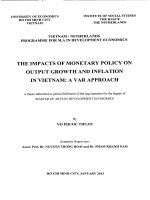
Impulse Response Analysis
Impulse response analysis examines that when the random disturbance term
changes by one standard deviation, how the endogenous variable will respond. The
impulse response figure shows the dynamic changes path of the endogenous
variable. Figure 2 represents the results of impulse response analysis on the basic
VAR model.

Figure 2: Response of SH Index to Cholesky One S.D. Innovations of US M2


The solid line is the response of Shanghai Composite Index to its own unexpected
changes. The response is positive and maximizes after 2 periods, but then the
response decreases gradually. The long-term response is close to 0. Therefore, this
result indicates that Chinese stock is influenced by its own unexpected in the short
run, but the influence is weak in the long term.
The dashed line is the response of Shanghai Composite Index to the shock from U.S.


54

Wei Wei

QE policy. When the U.S. M2 changed by one standard deviation, China stock had
negative response in the first period but the response became positive after the third
period. Then the response increases gradually and reaches the maximum at the ninth
period. After the ninth period, the response decreased. The long-term response is
close to zero. This means that the liquidity created by U.S. QE policy influences
China stock in the short and mid-term. But in the long term, the response disappears.
3.4
Variance Decomposition
The variance decomposition determines how much of the forecast error variance of
each of the variables can be explained by exogenous shocks to the other variables,
indicating the amount of information each variable contributes to the other variables
in the autoregression.
Table 5 represents the results of variance decomposition. Contribution rate from
U.S. M2 to SH Index maximized at the first period, reaching 4.0191%. Then it
decreases gradually and reaches 2.2679% at the 24th period. This means that the
liquidity created by U.S. QE policy influences the Chinese stock market at the short
term but decreases gradually. In the long term, the Chinese stock market is most
influenced by its own unexpected changes. There are two reasons for this

phenomenon. One is that the liquidity created by U.S. QE policy flows to the
Chinese stock market in the short term, but in the long term, the liquidity may flow
to other capital market such as real estate market. The other reason is that many
factors influence the Chinese stock market, such as the domestic economic situation.
In the long term, other factors may offset the influence of U.S. QE policy.


The Spillover Effects of U.S. Monetary Policy on the Chinese Stock Market

55

Table 5: Results of Variance Decomposition in the Basic VAR System

Period
S.E.
US M2
SH Index
1
0.057405
4.019087
95.98091
2
0.090389
3.817326
96.18267
3
0.111942
3.258371
96.74163
4

0.125710
2.884831
97.11517
5
0.134525
2.655328
97.34467
6
0.140230
2.515107
97.48489
7
0.143967
2.428069
97.57193
8
0.146441
2.372982
97.62702
9
0.148091
2.337493
97.66251
10
0.149198
2.314294
97.68571
11
0.149944
2.298961

97.70104
12
0.150446
2.288746
97.71125
13
0.150786
2.281902
97.71810
14
0.151016
2.277299
97.72270
15
0.151172
2.274196
97.72580
16
0.151277
2.272100
97.72790
17
0.151349
2.270683
97.72932
18
0.151397
2.269723
97.73028
19

0.151430
2.269074
97.73093
20
0.151452
2.268634
97.73137
21
0.151467
2.268336
97.73166
22
0.151477
2.268134
97.73187
23
0.151484
2.267998
97.73200
24
0.151489
2.267905
97.73210
Note: This table presents the variance decomposition ratio in the basic VAR system,
{ U.S. PPI, U.S. IP, U.S. CPI, U.S. M2, SH Index}.
3.5
The Dynamic Trend of Spillover Effect
In this section, I use rolling windows in the sample period to test the dynamic trend
of spillover effect. Since the time interval between adjacent rounds of QE policy is
about two years, I set the length of rolling windows as two years. The fixed-length

window rolls forward. The earliest month is removed each time when the next
month is added. Therefore, there are 52 windows in the sample period. The first
window is from January, 2008 to December, 2009, and the last window is from
April, 2012 to April, 2014.
By constructing the same VAR system and performing the Granger Causality test,
I calculate the F statistics of “U.S. M2 does not Granger Cause SH Index” in every
window. By comparing the F statistics in different windows, I analyze the dynamic
trend of spillover effect of U.S. QE policy on the Chinese stock market.


56

Wei Wei

Figure 3 represents the results of rolling tests. The solid line is the time series F
statistics of Granger Causality test in different windows. I find that the F statistics
fluctuate periodically. The F statistics are relatively large near the midpoint of each
round of QE policy. Moreover, the spillover effects are relatively larger in the first
two rounds than the last two rounds.

Figure 3: Dynamic Trend of the Spillover Effect
Note: This figure plots dynamic trend of the spillover effect of U.S. QE policy on
the Chinese stock market. The solid line is the time series F statistics of Granger
Causality test in different windows, and the dashed line is the 10% significant
threshold.

4. Potential Mechanisms
In this section, I run several tests to examine how U.S. QE policy influences the
Chinese stock market. It is challenging to provide definitive proof of potential
mechanisms, so the results are only suggestive.

4.1
Theoretical Analyses
4.1.1 Short-term Capital Flow
Since the Financial Crisis in 2008, the economies of developed countries recovers
slowly, while in developing countries such as China, India and Brazil, the economy
has better prospect. On the one hand, developing countries have raised interest rates
to cope with the inflationary pressure. For example, China has raised the deposit


The Spillover Effects of U.S. Monetary Policy on the Chinese Stock Market

57

and lending rates by 0.25% for five times from October, 2010 to July, 2011. The
spreads between US and developing countries appeal much capital to flow into
developing countries. On the other hand, since much capital flow into China, the
demand for RMB increased, thus the upward pressure on RMB increased, further
increasing the interest arbitrage space.
Under the background of interest rate spreads and expectations for appreciation of
RMB, international short-term capital flow will not only flow into the real economy,
but also flow into the Chinese stock market. Since the Split-share Structure Reform
in 2005, the scale of tradable shares in the Chinese stock market increases greatly,
thus enlarging the demand for capital. Therefore, the international short-term capital
flow induced by U.S. QE policy will influence the Chinese stock market. On the
other hand, most Chinese investors are speculators. They are easy to be influenced
by market sentiment and hearsay, thereby increasing the stock price fluctuation.
4.1.2 Monetary Policy Dependence
Since the reform and opening-up, the relationship between China’s economy and
global economy has become closer and closer. Therefore, shock from U.S. QE
policy may influence the China’s monetary policy.

First, Impossible Triangle Theory has proved that one country cannot realize fixed
exchange rate, free movement of capital and monetary policy independence at the
same time. According to the theory, under background of the fixed exchange rate,
with the level of capital flow increasing, the independence of Chinese monetary
policy will decrease.
Therefore, under the background of limited floating exchange rate and mandatory
exchange settlement in China, Chinese central bank cannot manage the money
supply completely and independently according to the economic development of
China.
Secondly, Chinese government gradually loosens control over capital flows. Since
1990s, much invisible capital has flowed into China. The invisible capital is greatly
influenced by domestic and international economic environment, and its existence
will affect the independence of Chinese monetary policy.
Therefore, the adjustment of US monetary policy will affect the money supply in
China, and then influence the Chinese stock market.
4.1.3 Stock Co-movement
First, Economic Fundamentals Theory proves that if there are same factors affecting
economies in different countries, the stock markets will change consistently when
external shocks occur. Changes in one economy will not only influence domestic
stock market, but also influence the economy and stock market in other countries.
Second, Market Contagion Hypothesis suggests that the relevance in different stock
markets can be attributed to the behaviors of investors. The changes of stock prices
in one market will influence investors’ sentiment and strategy in other markets.
Moreover, due to the time difference, investors can observe changes in other stock


58

Wei Wei


markets and then adjust their investment strategy in their own stock market.
Therefore, the opening price in one market may be affected by the closing price in
other markets, thereby causing the stock price co-movements.
4.2
Empirical Results
First, I test the effect of U.S. QE policy on the intermediary variables. I construct
the {U.S. PPI, U.S. IP, U.S. CPI, U.S. M2, China M2} and {U.S. PPI, U.S. IP, U.S.
CPI, U.S. M2, Chinese interest rate} VAR systems to test the effect of U.S. QE
policy on Chinese monetary policy, {U.S. PPI, U.S. IP, U.S. CPI, U.S. M2, China’s
short-term capital inflows} to test the effect on China’s short term capital flow, and
{U.S. PPI, U.S. IP, U.S. CPI, U.S. M2, S&P 500} to test the effect on U.S. stock
market.
Table 6 shows the results of Granger Causality test of the four VAR models. The
results show that U.S. M2 granger causes China M2, China’s short-term capital
flows and S&P 500.
Table 6: Results of the Granger Causality Test Between the USM2 and Intermediary
Variables

Null Hypothesis:
Obs
F-Statistic Prob.
ChinaM2 does not Granger Cause USM2
0.85494
0.4964
68
USM2 does not Granger Cause ChinaM2
4.72189
0.0023
USM2 does not Granger Cause ChinaRate
0.54419

0.4631
74
ChinaRate does not Granger Cause USM2
1.16585
0.2839
ChinaFlow does not Granger Cause USM2
2.5434
0.1155
71
USM2 does not Granger Cause ChinaFlow
5.19208
0.0258
S&P500 does not Granger Cause USM2
3.79516
0.1510
67
USM2 does not Granger Cause S&P500
1.69465
0.0050
Note: This table presents the results of the Granger causality test between the USM2
and four intermediary variables.
Figure 4 shows the results of the impulse response analyses on the four VAR models.
The results indicate that the influence of U.S. QE policy on China monetary policy
is relatively weak. The influence on China’s short-term capital flow is strong in the
short run but weak in the long run. As for the stock co-movement mechanism, the
result indicate that the U.S. QE policy has negative impact on U.S. stock market but
the effect turns positive in the mid and long run.


The Spillover Effects of U.S. Monetary Policy on the Chinese Stock Market


59

Figure 4: Response of the Intermediary Variables to Cholesky One S.D.
Innovations of US M2
Next, I test the effect of the intermediary variables on the Chinese stock market by
constructing {China M2, China’s short-term capital inflows, S&P 500 and SH Index}
VAR model.
Table 7 represents the results of Granger Causality test of the VAR model. I find
that under the significance level of 10%, China M2, China’s short-term capital
inflows, and S&P 500 granger cause SH Index.
Table 7: Results of the Granger Causality Test Between the Intermediary Variables
and SH Index

Null Hypothesis:
Obs F-Statistic Prob.
SH Index does not Granger Cause S&P500
33.8581 6.E-11
74
S&P500 does not Granger Cause SH Index
4.16597 0.0196
ChinaM2 does not Granger Cause SH Index
2.93248 0.0600
73
SH Index does not Granger Cause ChinaM2
7.82011 0.0009
ChinaFlow does not Granger Cause SH Index
0.24624 0.0155
70
SH Index does not Granger Cause ChinaFlow

4.44768 0.7825
Note: This table presents the results of the Granger causality test between the
intermediary variables and SH Index.


60

Wei Wei

Figure 5 shows the results of the impulse response analyses on the VAR model. I
find that SH Index is mostly influenced by itself. The three intermediary variables
only affect the Chinese stock market in the short term.

Figure 5: Response of SH Index to Cholesky One S.D. Innovations of Each
Intermediary Variable
Table 8 shows the results of variance decomposition of the VAR model. The results
indicate that China M2 has the greatest contribution rate among the three
intermediary variables. The second variable is S&P 500, and short-term capital
flows play the least role. The contribution rate of China M2 increases over time,
while the contribution rates of S&P 500 and short-term capital flows are relatively
stable.


The Spillover Effects of U.S. Monetary Policy on the Chinese Stock Market

61

Table 8: Results of Variance Decomposition for the Potential Mechanisms

Period

S.E.
ChinaM2 China Flow
S&P500
SH Index
1
0.052688
0.225537
6.411592
5.709843
87.65303
2
0.078480
5.089044
4.624777
5.570184
84.71600
3
0.095485
6.873424
3.132957
5.719491
84.27413
4
0.104579
7.723191
2.667224
5.826762
83.78282
5
0.109242

8.140824
2.606709
5.898505
83.35396
6
0.111492
8.354130
2.642382
5.943083
83.06040
7
0.112563
8.481688
2.680733
5.968560
82.86902
8
0.113074
8.566265
2.701038
5.982280
82.75042
9
0.113320
8.626539
2.708873
5.988920
82.67567
10
0.113439

8.670022
2.711018
5.991527
82.62743
11
0.113495
8.700665
2.711218
5.992005
82.59611
12
0.113520
8.721169
2.710969
5.991541
82.57632
13
0.113531
8.733844
2.710722
5.990862
82.56457
14
0.113535
8.740785
2.710555
5.990392
82.55827
15
0.113538

8.743849
2.710446
5.990357
82.55535
16
0.113540
8.744606
2.710362
5.990849
82.55418
17
0.113542
8.744322
2.710275
5.991873
82.55353
18
0.113545
8.743983
2.710168
5.993380
82.55247
19
0.113549
8.744336
2.710028
5.995288
82.55035
20
0.113553

8.745934
2.709846
5.997501
82.54672
21
0.113558
8.749179
2.709620
5.999914
82.54129
22
0.113564
8.754357
2.709350
6.002426
82.53387
23
0.113570
8.761661
2.709036
6.004938
82.52436
24
0.113578
8.771221
2.708683
6.007361
82.51273
Note: This table presents the variance decomposition ratio in the VAR system,
{China M2, China’s short-term capital inflows, S&P 500 and SH Index}.

Finally, I compare the effects through the three potential mechanisms. Table 8
summarizes the results of Variance Decomposition, and Table 9 summarizes the
direction of each mechanism. I find that the monetary policy dependence
mechanism is the most important mechanism through which U.S. QE policy
influence the Chinese stock market.
Table 9: Variance Decomposition Ratios of three potential mechanisms

Variance decomposition
ChinaM2 ChinaFlow
From U.S. M2 to intermediary variables
4.27%
2.10%
From intermediary variables to SH Index
8.77%
2.71%
Total influence
0.374%
0.057%

S&P 500
3.94%
6.01%
0.237%


62

ChinaM2
ChinaFlow
S&P 500


Wei Wei
Table 10: Comparison of Three Potential Mechanisms
From U.S. M2 to
From intermediary
Total influence
intermediary variables
variables to SH Index
Short-term
Long-term Short-term Long-term Short-term Long-term
＋
＋
＋
＋
＋
＋
＋
—
＋
—
＋
—
—
＋
＋
＋
—
＋

Note: This table compares the short-term and long-term influences through different

mechanisms.

5. Conclusion
Using the VAR methodology, I find that the U.S. QE policy has a significantly
positive effect on the Chinese stock market in the short term but the effect is in
significant in the long term. Then I examine three potential mechanisms through
which U.S. QE policy influences the Chinese stock market: short-term capital flow,
monetary policy dependence and stock co-movement. Using the variance
decomposition method, I find that the monetary policy dependence mechanism is
the most important one among all the three mechanisms, while the short-term capital
flow mechanism plays the least important role.

ACKNOWLEDGEMENTS. I acknowledge financial support from Tsinghua
University Tutor Research Fund.

References
[1] Bernanke, B. S., Boivin, J., & Eliasz, P. (2005). Measuring the effects of
monetary policy: a factor-augmented vector autoregressive (FAVAR)
approach. The Quarterly journal of economics, 120(1), 387-422.
[2] Canova, F. (2005). The transmission of US shocks to Latin America. Journal
of Applied econometrics, 20(2), 229-251.
[3] Dedola, L., Karadi, P., & Lombardo, G. (2013). Global implications of national
unconventional policies. Journal of Monetary Economics, 60(1), 66-85.
[4] Dornbusch, R. (1976). Expectations and exchange rate dynamics. Journal of
political Economy, 84(6), 1161-1176.
[5] Ehrmann, M., & Fratzscher, M. (2009). Global financial transmission of
monetary policy shocks. Oxford Bulletin of Economics and Statistics, 71(6),
739-759.
[6] Fleming, J. M. (1962). Domestic financial policies under fixed and under
floating exchange rates. Staff Papers, 9(3), 369-380.

[7] Ho, S. W., Zhang, J., & Zhou, H. (2018). Hot Money and Quantitative Easing:
The Spillover Effects of US Monetary Policy on the Chinese Economy. Journal
of Money, Credit and Banking, 50(7), 1543-1569.


The Spillover Effects of U.S. Monetary Policy on the Chinese Stock Market

63

[8] Homa, K. E., & Jaffee, D. M. (1971). The supply of money and common stock
prices. The Journal of Finance, 26(5), 1045-1066.
[9] Keran, M. W. (1971). Expectations, money, and the stock market (pp. 16-31).
Federal Reserve Bank of St. Louis.
[10] Kim, S. (2001). International transmission of US monetary policy shocks:
Evidence from VAR's. Journal of Monetary Economics, 48(2), 339-372.
[11] Lucas Jr, R. E. (1972). Expectations and the Neutrality of Money. Journal of
economic theory, 4(2), 103-124.
[12] Maćkowiak, B. (2007). External shocks, US monetary policy and
macroeconomic fluctuations in emerging markets. Journal of monetary
economics, 54(8), 2512-2520.
[13] Mann, T., Atra, R. J., & Dowen, R. (2004). US monetary policy indicators and
international stock returns: 1970–2001. International Review of Financial
Analysis, 13(4), 543-558.
[14] Mundell, R. A. (1963). Capital mobility and stabilization policy under fixed
and flexible exchange rates. Canadian Journal of Economics and Political
Science, 29(4), 475-485.
[15] Obstfeld, M., & Rogoff, K. (1995). Exchange rate dynamics redux. Journal of
political economy, 103(3), 624-660.
[16] Thorbecke, W. (1997). On stock market returns and monetary policy. The
Journal of Finance, 52(2), 635-654.

[17] Tobin, J. (1969). A general equilibrium approach to monetary theory. Journal
of money, credit and banking, 1(1), 15-29.
Appendix. Variable Definitions

Variable
USM2
SH Index
ChinaM2
ChinaRate
ChinaFlow
S&P 500
USPPI
USCPI
USIP

Definition
U.S. money supply M2
Shanghai Composite Index
China money supply M2
The one-year deposit and lending rate in China
The short-term capital inflows of China
S&P 500 Index
U.S. Producer Price Index
U.S. Consumer Price Index
U.S. Industrial Production Index