Bui Huu Phuoc • Pham Thi Thu Hong • Ngo Van Toan

Asset Price Volatility of Listed
Companies in the Vietnam Stock
Market
Bui Huu Phuoc(1) • Pham Thi Thu Hong(2) • Ngo Van Toan(3)
Received: 18 July 2017 | Revised: 12 December 2017 | Accepted: 20 December 2017

Abstract: This study aims to measure the volatility in asset
prices of listed companies in the Vietnam stock market. The
authors use models such as AR, MA and ARIMA combined with
ARCH and GARCH to estimate value at risk (VaR) and the results
generate relatively accurate estimates. In Vietnam, the stock
market has been through periods of wild fluctuations in security
prices and abnormal fluctuations cause many risks in investment
activities. Based on this empirical result, investors can approach
the method to determine asset price volatility to make proper
investment decisions.
Keywords: Asset price volatility, VaR, ARIMA - GARCH (1,1), risks.
jel Classification: C58 . G12 . G17.
Citation: Bui Huu Phuoc, Pham Thi Thu Hong & Ngo Van Toan (2017). Asset
Price Volatility of Listed Companies in the Vietnam Stock Market. Banking
Technology Review, Vol 2, No.2, pp. 203-219.

Bui Huu Phuoc - Email:
Pham Thi Thu Hong - Email:
Ngo Van Toan - Email:
(1), (2), (3)

University of Finance and Marketing;

2/4 Tran Xuan Soan Street, Tan Thuan Tay Ward, District 7, Ho Chi Minh City.

Volume 1: 149-292 | No.2, December 2017 | banking technology review

203


Asset price volatility of listed companies in the Vietnam stock market

1. Introduction
Since financial instabilities in the 1990s (Jorion, 1997; Dowd, 1998; Crouhy et
al., 2001), financial institutions have focused on modifying and conducting studies
through complex models to estimate market risks. The increased volatility in the
capital market encouraged research and field surveys to recommend and develop
proper risk management models. Managing risks in capital markets based on VaR
models have become academic topics receiving special attentions. VaR provides
answers to the questions of what the maximum value an investment portfolio can
lose under normal market conditions over a time horizon and with a certain degree
of confidence (RiskMetrics Group, 1996).
In an attempt to measure the accuracy of estimates of risk management models,
this study used a two-stage process to check each volatility estimation technique.
In the first stage, backtesting was conducted to examine the model’s accurate
statistics. In the second stage, this study used a forecasting assessment technique
to examine differences between the models. This study focused on out-of-sample
as an assessment criterion since one model, which might be incomplete to certain
assessment criteria, can still produce better forecasts for the out-of-sample
examples than predetermined models. This study shows that the GARCH model
is more agile, generates more complete volatility estimations, while providing all
coefficients, distribution assumptions and confidence degrees. Moreover, although
the utilisation of all available data represents a common practice in estimating the

volatility, the authors find that at least in some cases, a limited sample size can
generate more accurate estimates than VaR because it combines changes in the
business behaviour more effectively. The next section describes ARCH, GARCH
models, and assessment frameworks for VaR estimates. The authors also provide
preliminary statistics, explain procedures and present the result of empirical
surveys of estimation models for daily stock returns.

2. Literature Review
2. 1. Value at Risk
The volatility of a company’s asset prices is an important financial variable
because it measures risk levels of the company’s assets. Profits always come with
risks. The greater the risk is, the higher the profit is. Thus, the estimation of asset
price volatility of a company assists investors in measuring risk levels of the
company’s asset, producing estimations of the profit returned from investing in the
company to formulate investment strategies.

204 banking technology review | No.2, December 2017 | Volume 1: 149-292


Bui Huu Phuoc • Pham Thi Thu Hong • Ngo Van Toan

According to Hilton (2003), VaR was first used for stock companies listed in
the New York stock exchange (NYSE). Hendricks (1996) claims that VaR is the
maximum amount of money that an investment portfolio can lose over a given
time horizon with a certain confidence degree. Therefore, VaR describes a loss that
can happen due to the exposure to market risks over a given period at a certain
confidence level.
In the late 1990s, the US Securities and Exchange Commission dictated that
companies must report a quantitative proclamation about market risks in their
financial reports in order to provide investors with convenience. Since then VaR

has become a primary tool. At the same time, the Basel Committee on Banking
Supervision said that companies and banks can rely on internal VaR calculations
to establish their capital requirements. Therefore, if their VaR is relatively low, the
amount of money that they have to spend on risks that can be worse, can also be
low.
In Vietnam, the State Securities Commission issued a regulation on the
establishment and operation of the risking management system for fund
management companies in 2013. In this regulation, the State Securities Commission
referred to VaR and basic VaR calculations to help fund management companies
manage risk more efficiently. VaR is typically calculated for each day of the asset
holding period with a confidence of 95% or 99%. VaR can be applied to all liquid
categories, whose values are adjusted according to the market. All high liquidity
assets that have unstable values are adjusted according to the market with a
certain probability distribution rule. The most significant limitation of VaR is that
assumptions about market factors which do not change substantially during the
VaR period. This is a significant limitation because it caused the bankruptcy of a
series of investment banks in the world in 2007 and 2008 due to sudden changes in
the market conditions that exceeded extrapolated trends.
For investors, VaR of a financial asset portfolio is based on three key variables:
confidence degree, the period in which VaR is measured, and profit and loss
distribution during this period. Different companies have different demands for
the degree of confidence depending on their risk appetite. Investors with low-risk
appetite would like to have a high degree of confidence. Additionally, the degree
of confidence selected should not be too high when verifying the validity of VaR
estimates because if the degree of confidence is too high, e.g. 99%, VaR will be
higher. In other words, VaR is lower when loss probability is higher, requiring a
longer period to collect data to determine the validity of the test.
The period over which VaR is measured: one of the important factors for

Volume 1: 149-292 | No.2, December 2017 | banking technology review


205


Asset price volatility of listed companies in the Vietnam stock market

applying VaR is the time period. In different timeframes, a portfolio’s rate of return
fluctuates at different degrees. The volatility of a portfolio is greater when the period
is longer.
Profit/loss distribution during the VaR period: the profit/loss distribution line
represents the most important variable, which is also the most difficult to be defined.
Since the degree of confidence depends on risk tolerance of the investors, VaR is
higher when the degree of confidence is high. Investors with low risk acceptance
will formulate a strategy that can reduce the probability of worst scenarios.
The idea of Hendricks (1996) and Hilton (2003) is to calculate VaR of the
market asset price by indicating the maximum amount of money a portfolio can
lose due to the exposure to market risks over a certain period and with a given
degree of confidence. In this study, the left fractile of the return rate of the market
asset price is used to measure downside risks while the right fractile describes
upside risks, indicating that with the volatility of the return rate, investors may
suffer losses. Therefore, this method focuses on reducing highest risks that can be
seen in financial markets. This will help to generates more accurate estimates of
market risks.
2.2. Empirical Studies
Bao et al. (2006) examined the RiskMetrics model, the conditional autoregressive
VaR and the GARCH model with different distributions: normal distribution, the
historically simulated distribution, Monte Carlo simulated distribution, the nonparametrically estimated distribution, and the EVT-based (Extreme Value Theory)
distributions for such markets as Indonesia, Korea, Malaysia, Taiwan, and Thailand.
Their results indicate that RiskMetric and GARCH models with distributions such
as normal distribution, t-student distribution, and the generalised error distribution

(GED) can be accepted before and after the crisis while the EVT-GARCH behaves
better during the 1997-1998 financial crisis in Asia.
Mokni et al. (2009) examined GARCH family models such as GARCH.
IGARCH and GJR-GARCH were adjusted with normal distribution assumptions,
t-students and skewed t-students to estimate VaR of NASDAQ index during a stable
period of the US stock market from 01/01/2003 until 16/07/2008. The results show
that GJR-GARCH models perform better than GARCH and IGARCH models in
two stages.
Koksal & Orhan (2012) compared a list of 16 GARCH models in risk measure
VaR. Daily return data were collected from emerging markets (Brazil, Turkey) and
developed markets (Germany, USA) during the period from 2006 until the end of

206 banking technology review | No.2, December 2017 | Volume 1: 149-292


Bui Huu Phuoc • Pham Thi Thu Hong • Ngo Van Toan

August 2009. Applying both unconditional tests of Kupiec and conditional tests of
Christoffersen, the study shows that, on average, ARCH model performs the best,
followed by the GARCH model (1,1) while t-students distribution generates better
results than standard distribution.
Zikovic & Filer (2009) compared the VaR estimation between developed and
emerging countries before the 2008 - 2009 global financial crisis. Models used in this
study include moving average model, RiskMetric, historical simulation, GARCH,
filtered historical simulation, EVT using GPD and EVT-GARCH distribution. Data
include stock indexes in five developed markets (USA, Japan, Germany, France,
and England) and eight emerging markets (Brazil, Russia, India, South Africa,
Malaysia, Mexico, Hong Kong and Taiwan) from 01/01/2000 until 01/07/2010. The
results show that the best performing models were EVT-GARCH and historically
simulated models with updated market fluctuations.

Kamil (2012) used logarithm of rate of return WIG-20 in period 1999-2011
with different types of ARIMA-GARCH(1,1) to calculate VaR in short and long
term. The author concludes that the calculation of VaR is impacted by distribution
(normal distribution, t-student distribution, generalised error distribution-GED)
with the condition of rate of return and find the best model to calculate VaR with
chosen data.
Vo Hong Duc & Huynh Phi Long (2015) test the suitability of risk measure VaR
in Vietnam. The study uses 12 different models to estimate one-day VaR for stock
indexes in the VN-Index and HNX-Index exchanges during the period 2006 – 2014
at different risk levels. The results show that at the risk level of 5%, many estimation
models do not satisfy test conditions. In addition, Hoang Duong Viet Anh & Dang
Huu Man (2011), Vo Thi Thuy Anh and Nguyen Anh Tung(2011) studied risk
acceptance models with data collected from the stock market in Vietnam. These
studies were conducted by referring to parameters through such economic models
as AR, MA, combined with ARCH and GARCH.
Generally, in these studies, VaR is calculated by the parametric approach with
a main focus on GARCH models and its sub models. These studies show that
financial data series are complex and hardly follow standard distribution rules.
The estimation of financial time series data is suitable for ARIMA models ranging
from the original ARIMA model to extended models such as ARCH, GARCH,
and GARCH-M, GR-GARCH variants. ARCH models change in the conditional
variance, therefore making it possible to predict the risk level of an asset’s rate of
return. However, ARCH has some limitations. If ARCH effects have too many lags,
they will significantly reduce the degrees of freedom in the model and this become

Volume 1: 149-292 | No.2, December 2017 | banking technology review

207



Asset price volatility of listed companies in the Vietnam stock market

increasingly serious for short time series, which negatively affects estimation results.
Models assuming positive and negative shocks have the same level of effect on risks.
In practice, the price of a financial asset reacts differently to negative and positive
shocks. GARCH model was developed to partially overcome these limitations.

3. Methodology and Data
There are many approaches to VaR calculation which include nonparametric
and parametric approaches. The nonparametric approach was known for the
historically simulated model. However, one limitation of this method is that the
distribution of historical data will overlap in the future. The parametric approach
contains RiskMetrics and GARCH models. Within the scope of this article, the
authors use parametric approach through time series econometric models: AR,
MA and ARIMA combined with ARCH and GARCH.
3.1. Methodology
Methods used in this study included Box-Jenkins ARIMA and GARCH. First,
this study investigates the stabilisation of time series data by ADF method. The
next step is to examine the autocorrelation of the data. LB method is used to test
ARCH effects of financial data series. If the original data series do not stabilise, the
difference method is used to test whether the series are stationary. In this study, in
order to select a model, AIC standard is adopted. The results of GARCH model
estimates is used to predict the volatility of stock prices by VAR and post-test VAR
procedures via backtesting. Research data is the daily closing data of companies
listed on the Vietnamese stock market.
To apply Box-Jenkins ARIMA procedures to the stabilised time series, the
stabilised series is obtained by taking an appropriate degree of error. This leads
to the ARIMA (p, d, q) model where p is the autoregressive level, q stands for the
moving average order, and d represents the order of the stabilised series.
The ARIMA (p, d, q) is given as:

φp(B)(1-B)dyt = δ + θq(B)ut
where φp(B) = 1-φ1B -...φpBp is the process of pth autoregressive process; θq(B) =
1-θ1B -...θqBq is the qth moving average process; (1-B)d is the dth difference, B is the
backward shift operator of the differencing order and ut is white noise.
Previous studies have tested the effectiveness of GARCH model in explaining
the volatility in financial markets. These studies indicate that GARCH models

208 banking technology review | No.2, December 2017 | Volume 1: 149-292


Bui Huu Phuoc • Pham Thi Thu Hong • Ngo Van Toan

can identify and quantify volatility levels with long and fat tail distribution, and
volatility clustering often appearing in the financial data series.
The ARCH model is specifically developed to model and forecast conditional
variances. ARCH model was introduced by Engle (1982) while GARCH model was
proposed by Bollerslev (1986). These models have been widely used in economically
mathematic models, especially in the analysis of financial time series as in the
studies of Bollerslev et al. (1992, 1994). GARCH model is more general than ARCH
model. GARCH (p, q) model is given as:

rt = µ + ε tσ t

q
p
 2
2
σ
ω
α

ε
β jσ t2− j
=
+
+
∑
∑
i t −i
 t
i =1
j =1

rt = µ + ε model;
in which p is the order ofGARCH
q is the order of ARCH model; (p, q)
tσ t
 2
2
2
is the number of lags.
=
+
+
σ
ω
αε
βσ
 t
rtt−1= µ + εtt−σ1 t
The εt error is assumed to follow a specific qdistribution

rules with a mean
p
 2
2
2
VaRvariance
t = ασ t σ . =r ωand
value of 0 and the conditional
μ
reflect
the
value and
α
ε
β
σ
+
+
t− j
 t t ∑ i t −i ∑ j average
i
1
j
1
=
=

return. μ is positive and quite small.
ω, β , αi are parameters of the model and also
VaRtupside = µt j+ ασ

t
the proportion of the coefficients whose
assumed to be non-negative.
µ + εare
rt =lags
tσ t

dowside
2
2
2
According to Floros (2008), VaR
ω value will
α + β are forecasted
= −σµbe
−quite
ασ small and
t
t t = ω +tαε t −1 + βσ t −1
to be smaller than 1 and to be relatively identical, in which β > α. This explains
1 loss > VaR
VaRint =the
ασprevious
for the fact that news about Ithe
volatility
period can be measured
t
t+1
0
loss

≤
VaR
based on ARCH coefficient . Also, the estimate
upside clearly indicates the sustainability
VaRt
= µt + ασ t
of the volatility when experiencing economic
shocks
or the impact of events on the
dowside
volatility.
VaRt
= − µt − ασ t
One important point of GARCH models is estimating these parameters using
1 loss > VaR
It+1
an appropriate maximum estimation method.
According to many studies, among
0 loss ≤ VaR
µ + εmodel,
rt =(p,q)
tσ t
sub-models of the general GARCH
GARCH (1,1) is the most effect

q
p
model because it generates most accurate
estimates
2

2 (Floros,22008).
σ
ω
α
ε
β jσ t − j
=
+
+
∑
∑
t
i
t
i
−
µsimplest
µ+ +ε tεσtσt t form of GARCH model is GARCH (1,1)
rThe
t r=
t =
and it is given as follow:
i =1
j =1


q q
p p
 2 2
2 2

2 2
σσt t= =ωω+ +∑∑ααiεitε−it −+i +∑∑β βjσjσt − tj− j rt = µ + ε tσ t
i
1
i
1
j
1
j
1
=
=
=
=

 2
2
2
σ t = ω + αε t −1 + βσ t −1
rt r=t =µµ+ +ε tεσtσt t
 2 2
VaRt = ασ the
2 2
t
=ωω+ +αεαε
βσ
βσt2−1t2−1 are respectively
which
and
squared return and the conditional

σinσt t=
t −1t −+
1+
upside
variance of the day before.
= µt + ασ t
t
ασt t obvious advantageVaR
VaR
VaR
=ασ
t =
t most
The
of GARCH model compared to ARCH is that
upside
upside
VaRtdowside = − µt − ασ t
VaR
VaR
= =µµ+ +ασ
ασ

{

{

t t

t t


t t

{

1 lossDecember
> VaR
dowside
dowside
2017 | banking technology review 209
It+1
VaR
VaR
= =− −µtµ−Volume
ασ
ασt t 1: 149-292 | No.2,
t t
t −
0 loss ≤ VaR


rt = µ + ε tσ t

Asset price volatility of listed companies
stock market
σ
+ εVietnam
r =inµthe
t


t

tq

p

rt = µ +εtσσt 2 = ω +q α ε 2 +p β σ 2
∑ i t −i ∑ j t − j
 2q t

σt = ω +2 ∑i =αp1 iε t2−i +2 ∑j =β1 jσ t2− j
 2

ω+GARCH(1,1)
α iε t −i i+=1 ∑ β(Engle,
ARCH(q) is infinite equals
∑
jσ t − jj =1 1982; Bollerslev, 1986). If
σ t =to
i
1
j
1
=
=

r
=
+
µ

ε
σ
t is large),
t t it can affect results of the estimate
ARCH model has too many lags(q
rt σ= 2µ=+ωε t+σαε
2
2
given a significant decrease
oft freedom
t −1 + βσ in
t −1 the model.
+εtdegree
σ2 tt
rt =inµthe
2
2
ω + αε2t −1 + βσ
σ t =to
 2 (2009),
t −1
In the study of Dmitriy
αε t2−1=+calculate
βσ t −1 VaR, formulas of upside VaR and
σ t = ω +VaR
ασ
t
t
downside VaR on the stock exchanges
are given as follows:

VaRt = ασ
t
upside
ασ
VaR
=

• VaR formula:
t
t
VaR
= µt + ασ t
t
upside

• Upside VaR formula:
VaR
=
µt + ασ t
t
upside
VaR
=
+
µ
ασ
dowside
t
t
t


• Dowside VaR formula: VaRt
= − µt − ασ t
VaRtdowside
− ασ t
= =µ −+µεtwith
ofrt return
in which μt is the expected
rate
of the stock; α is the
tσ t conditions
dowside
VaRt
= −µ1t −loss
ασ>t VaR
q
p
I
quantile for normal distribution which
of the GARCH
t+1 2 is often used2 for residuals
2
1 loss
VaR
loss
≤ VaR
σ0tthe
=> ω
+ ∑ α iε t −i variance
+ ∑ β jσseries

It+1> σVaR
t− j
model on the stock exchange;
and
is
conditional
of the asset.
1 loss

t0 loss ≤ VaR
It+1
i =1
j =1

0
loss
≤
VaR
Many researchers show their interest in accurate estimates of future risks. In
an attempt to evaluate the quality of
models should be rechecked
= µ estimates,
+ ε tσ t
rtVaR

by appropriate methods. Backtesting is2 a statistical
process
for comparing actual
2
2

σ t = ω + αε t −1 + βσ t −1
profits and losses with corresponding
VaR estimates. For example, if the degree of
confidence is used to calculate the complete
VaR of VaR methods, especially when a
VaRt = ασ
t
few methods are compared. Two alternative methods to VaR methods that are often
upside
used in studies include: the basis of VaR
accuracy
=tests
µt +and
ασ tloss functions.
t
VaR backtesting model is implemented by calculating the number of losses
dowside
VaR
= − µtof− VaR
ασ t violations can be defined
which are greater than VaR estimates.
The
t number
as follows:

{

{{

It+1


{

1 loss > VaR
0 loss ≤ VaR

A risk model should be enhanced to estimate the probability (p) of VaR
violations. VaR violation probability relies on the VaR coverage ratio. Processes of
a risk model determine exactly as a series of random coin tosses (Christoffersen &
Jacobs, 2004).
3.2. Data
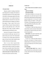
We randomly selected two companies listed on the Ho Chi Minh City stock
exchange (HOSE): a financial company and a non-financial company for the test.
This helped us to simplify the research process and not to affect the scientific nature
of the research. Collected data are daily closing prices of listed companies on
the market. Closing price data were collected from 21/11/2006 until 04/12/2015.
Specifically, closing prices of ACB were collected from 21/11/2006 and closing
prices of AAA were gathered from 15/07/2010. ACB is the stock code of the
Asia commercial bank and AAA is the stock code of An Phat plastic and green

210 banking technology review | No.2, December 2017 | Volume 1: 149-292


Bui Huu Phuoc • Pham Thi Thu Hong • Ngo Van Toan

environment company. Daily rates of return of closing prices were calculated as
follows:
rt = ln(Pt /Pt-1)

-.1


-.1

-.05

-.05

0

.05

re_ACB

.05
0

re_AAA

.1

.1

.15

.15

in which: Pt is the stock price at the closing time on the tth exchange date; Pt-1
is the closing price of the stock on the t-1th date.
Figure 1 shows that the return rate of AAA and ACB stocks fluctuated over
time with prices going up and down. There is volatility clustering in the series.


0

500

1000

STT

1500

2000

2500

0

500

1000

STT

1500

2000

2500

Figure 1. Daily rates of return of AAA and ACB (21/11/2006-04/12/2015)


Analysis results of the basic statistical values show significant fluctuations in
the series. Kurtosis measures peaked or flat degrees of a distribution in comparison
with a normal distribution whose kurtosis is 0. A distribution has a peaked shape
when the kurtosis is positive and a flat shape when the kurtosis is negative. A kurtosis
of more than 3 show that the “peakedness” of the peaked distribution is greater
than a normal distribution. Stationary test reveals that both AAA and ACB series
stabilised at the significant level of 1%. Jarque-Bera test shows that the averages of
the two series have non-normal distributions. ARCH effect tests uses Ljung-Box Q
test lags (10) for the squared residuals of the return rate with a significant level of
1%. This indicates that GARCH (1,1) can be applied to these data series.
Table 1. Descriptive Statistics
RE_AAA

RE_ACB

Avarage

-0.0005

-0.0001

Standard
Deviation

0.0294

0.0233

Volume 1: 149-292 | No.2, December 2017 | banking technology review


211


Asset price volatility of listed companies in the Vietnam stock market

RE_AAA

RE_ACB

Skewness

0.0391

0.1088

Kurtosis

3.9788

6.7684

JB test

53.9525
(0.000)

1333.414
(0.000)


Sample

1.343

2.246

ADF test

-34.2351
(0.000)

-41.0204
(0.000)

LB-Q (10)

19.9636
(0.000)

52.6971
(0.000)

4. Empirical Results

0.15
0.10
0.005
-0.05

-0.050


Autocorrelations of re_acb

0.05
0.00
-0.05
-0.10

Autocorrelations of re_aaa

0.10

• GARCH model estimation
A GARCH model includes two equations. The first one is an average equation
while the second one is a variance equation. The estimate results obtained from the
research data are represented in Figure 2.

0

10

20

30

Lag
Bartllet’s formula for MA(q) 95% confidence bands

40


0

10

20

30

40

Lag
Bartllet’s formula for MA(q) 95% confidence bands

Figure 2. Autocorrelation results of AAA and ACB stocks

Results obtained from the Box-Jenkins method show that AAA and ACB data
series are significant (Figure 2). Therefore, in this study, ARIMA can be applied
in the mean equation for ARCH effects. Data experiment allow us to select lags
of AR (1) and MA (1). Outlier observations have null values, suddenly falling to
0. d is obtained through Jarque-Bera and ADF methods, indicating that the series
stabilises at level 1.
The comparison between the values of AIC and Log likelihood from GARCH
(1,1), GARCH (2,2), GARCH (1,2) và GARCH (2,1) in Table 2 show that GARCH
(1,1) provides the smallest AIC and the largest Log likelihood.

212 banking technology review | No.2, December 2017 | Volume 1: 149-292


Bui Huu Phuoc • Pham Thi Thu Hong • Ngo Van Toan


Table 2. Results of GARCH model of AAA
Parameter

GARCH (1,1)

GARCH (2,2)

GARCH (2,1)

GARCH (1,2)

AR (1)

0.8650***
(4.10)

0.8380***
(4.65)

0.8630***
(4.81)

0.9080***
(5.23)

MA (1)

-0.8470***
(-3.77)


-0.8150***
(-4.27)

-0.8440***
(-4.44)

-0.8960***
(-4.86)

α1

0,1460***
(6.77)
0.1330***
(5.94)

α2
β1

0.7990***
(30.63)

0.1100***
(6.95)
0.840***
(37.65)

0.7760***
(22.37)


β2
α0

0.2520***
(7.190)

0.00005***
(5,24)

0.0001***
(4.96)

0.6630***
(16.83)
0.00004***
(4.76)

0.0001***
(5.75)

N

1.343

1.343

1.343

1.343


AIC value

-5876.8000

-5806.0000

-5841.2000

-5872.9000

BIC

-5845.5000

-5774.8000

-5810

-5841.7000

Log likelihood

2944.3800

2909.0250

2926.6120

2942.4610


t statistics in parentheses
* p<0.05, ** p<0.01, *** p<0.001.

Standardised results of AIC and Log likelihood of Table 3 show that the selected
model for estimations in this research is GARCH (1,1). Selection criteria of the
model are the smallest AIC and the largest Log likelihood.
Table 3. Results of GARCH model of ACB
Parameter

GARCH (1,1)

GARCH (2,2)

GARCH (2,1)

GARCH (1,2)

AR (1)

-0.9650***
(-54.49)

0.9270***
(34.78)

0.2490
(1.12)

-0.7880***
(-5.43)


MA (1)

0.9780***
(71.56)

-0.8710***
(-27.73)

-0.1490
(-0.66)

0.8180***
(6.04)

α1

0.2950***
(14.51)

α2

0.249***
(17.18)
0.31700***
(13.84)

0.2080***
(12.21)


Volume 1: 149-292 | No.2, December 2017 | banking technology review

213


Asset price volatility of listed companies in the Vietnam stock market

Parameter

GARCH (1,1)

β1

0.7290***
(59.08)

GARCH (2,2)

GARCH (2,1)

GARCH (1,2)

0.7810***
(56.97)
0.7560***
(107.06)

0.6860***
(41.52)


β2
α0

0.00001***
(18.94)

0.00002***
(16.69)

0.00002***
(14.24)

0.00001***
(25.41)

N

2.246

2.246

2.246

2.246

AIC value

-11805.2000

-11572.4000


-11590.3000

-11708.9000

BIC

-11770.9000

-11538.1000

-11556.0000

-11674.6000

Log likelihood

5908.59000

5792.2150

5801.1640

5860.4490

t statistics in parentheses
* p<0.05, ** p<0.01, *** p<0.001.

0


.002

.004

.006

Figure 3 describes trends of the conditional variance of the return rate series of
AAA and ACB, representing the volatility degree of corresponding data series. The
volatility degrees of the two series are different and the series fluctuate significantly,
in which the volatility in the return rate of AAA is greater. Volatility scale not only
represents highest risks during each period but can also help us predict market
volatility and relevant risks.

500

1000

1500

2000

2500

0

STT
myvariance_aaa

myvariance_acb


Figure 3. Conditional variance of the return rates of AAA and ACB

• Upside and downside VaR calculation
Figure 4 reveals that VaR estimates at the confidence degrees of 95% and 99%
creates series of return rate of AAA and ACB. Asset fluctuations are relatively
significant, and this indicates that with strong volatility, investors holding the asset
will face very high risks.

214 banking technology review | No.2, December 2017 | Volume 1: 149-292


Bui Huu Phuoc • Pham Thi Thu Hong • Ngo Van Toan

.16

.20

.12

.15

.08

.10

.04

.05

.00


.00

-.04

-.05

-.08

-.10

-.12

-.15

250

500
RE_AAA

750
VAR99_AAA

1000

1250

250

500


750

RE_ACB

VAR95_AAA

1000

1250

1500

VAR95_ACB

1750

2000

VAR99_ACB

Figure 4. Calculation of VaR (95%) và VaR (99%)

Results in Figure 5 shows that the confidence degree of 99% provides more
accurate estimates than 95% with fewer violations. Next, we consider the estimation
period of 10 days and the degrees of confidence of 95% and 99%, generating accurate
results. The results indicate that volatility in AAA’s asset is more complex and larger
than those of ACB during the observed period.
.20


.15

.15

.10

.10
.05

.05

.00

.00
-.05

-.05

-.10
-.10
-.15

-.15

250

500
RE_AAA
UPVAR99_AAA
DOWVAR95_AAA


750

1000
UPVAR95_AAA
DOWVAR99_AAA

1250

-.20

250

500

750

1000

RE_ACB
DOWVAR95_ACB
UPVAR99_ACB

1250

1500

1750

2000


DOWVAR99_ACB
UPVAR95_ACB

Figure 5. VaR 95% and VaR 99% (Upside/Downside)

• Analysis of the estimation process
Figure 6 show that VaR estimation during a period of 10 days is accurate at the
degrees of confidence of 95% and 99% for both AAA and ACB. Violation rate is 0%
during this period and this result has been confirmed since the post test results.
• Backtesting
Backtesting was conducted on ACB’s data series with 2.247 samples. Tests within
the sample was completed with 2.237 samples during the period from 21/11/2006
until 20/11/2015. Out of sample tests were performed for the 10 remaining samples
during the period from 23/11/2015 until 04/12/2015 (Table 4).

Volume 1: 149-292 | No.2, December 2017 | banking technology review

215


Asset price volatility of listed companies in the Vietnam stock market

.08

.06

.06

.04


.04
.02

.02
.00

.00

-.02

-.02

-.04
-.04

-.06
-.08

1

2

3

4

5

6


RE_AAA
UPVAR99_AAA
DOWVAR95_AAA

7

8

9

10

UPVAR95_AAA
DOWVAR99_AAA

11

-.06

1

2

3

4

5


UPVAR99_ACB
RE_ACB
DOWVAR95_ACB

6

7

8

9

10

UPVAR95_ACB
DOWVAR99_ACB

Figure 6. Actual rates of return and 10-day VaR with the confidence degrees
of 95% and 99%
Table 4. Post test results
ACB (21/11/2006-20/11/2015)
VaR 95%

VaR 99%

170 violations (7.57%)

73 violations (3.25%)

AAA (15/07/2010-20/11/2015)

125 violations (9.33%)

38 violations (2.83%)

Similarly, AAA’s data series with 1.344 sample were divided into two periods.
Within sample tests were conducted on 1.334 samples from 15/7/2010 until
04/12/2015. Out of sample test were conducted on the 10 remaining samples from
23/11/2015 until 04/12/2015.
Backtesting results within the sample show that the numbers of violations at
different degrees of confidence are different. In contrast, out of sample backtesting
results (during the period from 23/11/2015 until 04/12/2015) provide a violation
rate of 0% for both AAA and ACB’s series.

5. Conclusion
The results of this study indicate that given the volatile nature of the financial
data series, it is necessary to select an appropriate measuring tool. Experimental
studies on AR, MA, and ARIMA models in combination with ARCH and GARCH
allow us to estimate VaR. Post-test procedures show that estimate results are
reliable. VaR provides predictions of maximum losses on the stock during a certain
period and at a predetermined degree of confidence. In other words, VaR provides

216 banking technology review | No.2, December 2017 | Volume 1: 149-292


Bui Huu Phuoc • Pham Thi Thu Hong • Ngo Van Toan

a scientific basis for us to determine whether risks facing investors are within
allowable limits. This allows investors to recognise the safety of holding assets on
the market. In addition, investors can use available data and GARCH economic
model to determine VaR for their assets. Investors will be able to decide whether to

continue holding current assets or not.
This study was conducted in an attempt to measure the volatility degrees in
assets of listed companies on the stock exchange in Vietnam. Estimate results of
the GARCH model show that the two data series of AAA and ACB is significant
for GARCH (1,1). This result is consistent with requirements from AIC and
Log likelihood standards of econometric models. Post-test results indicate that
GARCH (1,1) can recognise and quantify fluctuations with long-tailed and
thick-tailed distributions which fluctuate according to clusters in the financial data
series. Post-test results of the 10-day estimates generates perfectly accurate results
at the two degrees of confidence in comparison with the actual results. Upside and
downside cases of the model is influenced by the selection of the estimated period.
One important factor of the financial data series is that the distribution of data
leads to the accuracy of the model estimate. Most financial data have long-tailed
and thick-tailed distributions. From the above-mentioned experimental results,
the authors hope to support risk managers in making decisions and solutions to
minimize risks.

References
Bao, Y., Lee, T. & Saltoglu, B. (2006). Evaluating VaR Models in Emerging Markets: A
Reality Check. Journal of Forecasting, vol. 25, no. 2, pp. 101-128.
Bollerslev, T. (1986). Generalized autoregressive conditional heteroskedasticity.
Journal of Econometrics, no. 31, pp. 307-27.
Bollerslev, T., Chou, R. & Kroner, K. (1992). ARCH modeling in finance: a review of
theory and empirical evidence. Journal of Econometrics, no. 52, pp. 5-59.
Bollerslev, T., Engle, R. & Nelson, D. (1994). ARCH model, Engle R. and McFadden, D.
L., Handbook of Econometrics vol. IV, Elsevier Science B.V., NorthHolland, pp. 2961-3031.
Box, G. E. P. & Jenkins, G. M. (1976). Time Series Analysis: Forecasting and Control,
San Francisco: Holden-Day.

Volume 1: 149-292 | No.2, December 2017 | banking technology review


217


Asset price volatility of listed companies in the Vietnam stock market

Christoffersen, P. & Jacobs, K. (2004). The importance of the loss function in option
valuation. Journal of Financial Economics, vol. 72, no. 2, pp. 291-318.
Crouhy, M. Galai, D. & Mark, R. (2001). Risk Management, McGraw Hill, New York.
Danielsson, J. (2002). The emperor has no clothes: Limits to risk modelling. Journal of
Banking & Finance, vol. 26, no. 7, pp. 1273-1296.
Dmitriy, P. (2009). Value at Risk Estimation and Extreme Risk Spillover between Oil
and Natural Gas Markets. Department of Economics, Central European University, pp. 1-61.
Dowd, K. (1998). Beyond Value at Risk: The new science of risk management. John
Wiley & Sons, New York.
Engle, R. F. (1982). Autoregressive Conditional Heteroscedasticity with Estimates of
Variance of United Kingdom Inflation. Econometrica, vol. 50, no. 4, pp. 987-1008.
Floros, C. (2008). Modelling volatility using GARCH models: evidence from Egypt
and Israel. Middle Eastern Finance and Economics, vol. 2, pp. 31-41.
Hendricks, D. (1996). Evaluation of value-at-risk models using historical data, Federal
Reserve Bank of New York. Economic Police Review, vol. 2, pp. 39-70.
Hilton, G. A. (2003). Value at Risk. Theory and Practice. New York.
Hoang Duong Viet Anh & Dang Huu Man (2011). Chat luong du bao rui ro thi
truong cua cac mo hinh Gia tri chiu rui ro – nghien cuu thuc nghiem tren danh muc
chi so VN-Index. Tap chi Nghien cuu Kinh te, so 397, trang 19-27. (The quality of market
volatility forecasts implied by Value-at-Risk models - empirical evidence from VN –
index. Economic Studies, no. 397, pp. 19-27.)
Jorion, P. (1997). Value at Risk: The new benchmark for controlling derivatives risk,
McGraw Hill, New York.
Kamil, M. (2012). Arima-Garch models in estimating market risk using value at risk

for the WIG20 Index. The Quarterly "e-Finanse", vol. 8, no. 2, pp. 25-33.
Köksal, B. & Orhan, M. (2012). Market risk of developed and developing countries
during the global financial crisis. />Mokni, K., Mighri, Z. & Mansouri, F. (2009). On the effect of subprime crisis on Value
at Risk estimation: GARCH family models approach. International Journal of Economics
and Finance, vol. 1, no. 2, pp. 88-104.
RiskMetrics Group (1996). RiskMetrics – Technical Document, New York: J.P. Morgan/
Reuters.

218 banking technology review | No.2, December 2017 | Volume 1: 149-292


Bui Huu Phuoc • Pham Thi Thu Hong • Ngo Van Toan

Vo Hong Duc & Huynh Long Phi. (2015). Kiem dinh su phu hop cua cac mo hinh uoc
tinh gia tri rui ro (VaR) tai Viet Nam. Tap chi Cong nghe Ngan hang, so 115, trang 3-15.
(Suitability tests of value at risk (VaR) estimation models in Vietnam. Banking Technology
Journal, no. 115, pp. 3-15)
Vo Thi Thuy Anh & Nguyen Anh Tung (2011). Do luong rui ro thi truong cua danh
muc chi so VN-Index bang mo hinh gia tri chiu rui ro. Tap chi Phat trien Kinh te, so
247. (Measuring market risks of VN-Index by value at risk models. Economic development
journal, no. 247).
Zikovic, S. & Filler, R. K. (2009). Hybrid Historical Simulation VAR and ES: Performance
in Developed and Emerging Markets. CESifo Working Paper Series, no. 2820, pp. 1-39.

Volume 1: 149-292 | No.2, December 2017 | banking technology review

219