Turkish Journal of Earth Sciences
/>
Research Article

Turkish J Earth Sci
(2016) 25: 19-45
© TÜBİTAK
doi:10.3906/yer-1501-36

Late Quaternary paleoceanographic evolution of the Aegean Sea: planktonic
foraminifera and stable isotopes
Ekrem Bursin İŞLER, Ali Engin AKSU*, Richard Nicholas HISCOTT
Department of Earth Sciences, Centre for Earth Resources Research, Memorial University of Newfoundland, St. John’s,
Newfoundland, Canada
Received: 29.01.2015

Accepted/Published Online: 19.11.2015

Final Version: 01.01.2016

Abstract: Aspects of the paleoclimatic and paleoceanographic evolution of the Aegean Sea since ~130 ka are revealed by quantitative
variations in planktonic faunal assemblages, the δ18O and δ13C isotopic composition of benthic and planktonic foraminifera, and
Mg/Ca ratios in planktonic foraminifera extracted from five 6–10-m-long piston cores. Independent sea surface temperature (SST)
estimates obtained using planktonic foraminiferal transfer functions and the Mg/Ca ratios show excellent agreement, with r2 correlation
coefficients of 0.92–0.95. Planktonic foraminiferal assemblages are similar, through time, across several deep basins, suggesting that
major changes must have occurred in near synchroneity across the Aegean Sea. The data suggest that sapropels S3, S4, and S5 were
deposited under a stratified water column during times of increased primary productivity and the development of a deep chlorophyll
maximum layer. Under such conditions, oxygen advection via intermediate water flow must have been significantly reduced, in turn
implying bottom water stagnation. Sapropel S1 lacks a deep phytoplankton assemblage; this faunal contrast between S1 and older
sapropels indicates that S1 must have been deposited in the absence of a deep chlorophyll maximum layer.
Cluster analysis shows a consistent coupling of Globigerina bulloides with Globigerinoides ruber during times of nonsapropel deposition,

interpreted to require a stratified euphotic zone composed of a warm, nutrient-poor upper layer and a cooler, nutrient-rich lower layer.
The covariation of these two species suggests increased river runoff that controlled the fertility and stratification of the surface waters.
Key words: Sapropel, planktonic foraminifera, SST, oxygen and carbon isotopes, Mg/Ca ratios, Quaternary, paleoclimate,
paleoceanography, Aegean Sea

1. Introduction
Planktonic foraminifera are powerful indicators of
water-mass characteristics in Pleistocene–Recent
paleoceanographic studies (e.g., Rohling et al., 2004).
Qualitative and quantitative studies show that planktonic
foraminifera have both geographic and water-depth
preferences, occupying distinct ecological niches
controlled by the water-mass properties, and upwelling
(e.g., Sautter and Thunell, 1991). Variations in oxygen and
carbon isotopic compositions and trace-element ratios
(e.g., Mg/Ca) in foraminiferal tests are reliable indicators of
sea-surface and bottom-water temperatures and salinities,
as well as the availability of food in the water column
(e.g., Lea et al., 2003; Rohling et al., 2004; Geraga et al.,
2005). Temporal changes can be tracked using downcore
variations of planktonic foraminiferal assemblages, with
distinctive assemblages assigned to separate ‘ecozones’
(e.g., Capotondi et al., 1999).
Many species of planktonic foraminifera host a variety
of photoautotrophs, including dinoflagellates, diatoms,
*Correspondence:

green algae, red algae, chrysophytes, and prymnesiophytes;
these symbiont-bearing planktonic foraminifera are better
adapted to a wider range of light conditions (e.g., colour

spectrum) and water depths in the oceans (Bé et al., 1982,
Hemleben et al., 1989, Edgar et al., 2013). The symbiont
plays a critical role in nutrition, reproduction, calcification,
growth, and longevity of the host organism (Edgar et al.,
2013). Symbiont-bearing planktonic foraminifera are
widespread and abundant across the euphotic zone in
subtropical and tropical oceans where food concentrations
and water temperatures and salinities can show large
vertical variations. Distinct planktonic foraminiferal
assemblages occur in such environments, largely
controlled by the specific temperature, salinity, nutrient,
and dissolved oxygen preferences of the constituent species
(Hemleben et al., 1989). Symbiont-bearing planktonic
foraminiferal species often show diurnal and ontogenetic
vertical migration patterns in the water column, and sink
into deeper waters during reproduction (Hemleben et

19


İŞLER et al. / Turkish J Earth Sci
al., 1989). In contrast, nonsymbiont-bearing planktonic
foraminiferal species, such as Neogloboquadrina dutertrei,
G. bulloides, and Globorotalia inflata, are not restricted to
the euphotic zone and are often found at greater depths in
the oceans (Bé et al., 1982, Hemleben et al., 1989).
There has been particular interest in the planktonic
foraminifera species G. ruber (white), which indicates
warm/oligotrophic summer mixedlayer conditions (e.g.,
Rohling et al., 1993; Reiss et al., 1999); Neogloboquadrina

pachyderma (dextral) and N. dutertrei, which are
intermediate water dwellers and may suggest shoaling
of the pycnocline into the base of the euphotic layer to
create a distinct deep chlorophyll maximum; G. bulloides,
which indicates eutrophic surface waters such as seen
in upwelling zones, and G. inflata and/or Globorotalia
scitula, which reflect a cool, homogeneous, and relatively
eutrophic winter mixed layer (Reis et al., 1999; Rohling et
al., 2004).
This paper uses planktonic foraminiferal assemblages,
δ18O records in planktonic and benthic foraminifera, and
Mg/Ca ratios in planktonic foraminiferal tests extracted
from five piston cores from the Aegean Sea. Objectives are
(i) to delineate the Late Quaternary paleoceanographic
evolution of the region, with special emphasis on the
determination of sea-surface temperature and salinity
variations during the accumulation of organic-rich
sediments (i.e. sapropels and sapropelic muds, Kidd et
al., 1978) and nonsapropelic background sediments and
(ii) to examine temporal and spatial variations in the
characteristics of the water column, in particular the
degree of stratification and temporal variations in the
depth and strength of the pycnocline. Little has been
published about sediments older than 20–28 ka in the
Aegean Sea (e.g., Casford et al., 2002; Geraga et al., 2008,
2010). Therefore, the paleoclimatic and paleoceanographic
history of this important gateway between the Black Sea
and the eastern Mediterranean Sea is, to a large extent,
limited to conditions following the last glacial maximum
(LGM). The core data presented in this paper provide a

much needed record of Aegean Sea paleoclimate and
paleoceanography prior to the LGM, in particular before
Marine Isotopic Stage (MIS) 2.
1.1. Seabed morphology and hydrography of the Aegean
Sea
The Aegean Sea is a shallow elongate embayment that forms
the northeastern extension of the eastern Mediterranean
Sea (Figure 1). To the northeast, it is connected to the Black
Sea through the straits of Dardanelles and Bosphorus and
the intervening small land-locked Marmara Sea. In the
south, the Aegean Sea communicates with the eastern
Mediterranean Sea through several broad and deep straits
located between the Peloponnesus Peninsula, the Island
of Crete, and southwestern Turkey (Figure 1). The Aegean

20

Sea is divided into three physiographic regions (italics): the
northern Aegean Sea, including the North Aegean Trough;
the central Aegean plateaux and basins; and the southern
Aegean Sea, including the Cretan Trough.
The dominant bathymetric feature in the northern
portion of the Aegean Sea is the 800–1200-m-deep
depression known as the North Aegean Trough. It includes
several interconnected depressions and extends WSW–SW
from Saros Bay, widening toward the west (Figure 1). The
central Aegean Sea is characterized by a series of shallower
(600–1000 m), mainly NE-oriented depressions and
their intervening 100–300-m-deep shoals and associated
islands (Figure 1; Yaltırak et al., 2012). Five cores were

collected from the central Aegean Sea, specifically from
the North Skiros, Euboea, Mikonos, and North and South
Ikaria basins (Figure 1). Regional studies have shown
that normal faulting and strike-slip faulting are the two
dominant mechanisms controlling seabed morphology in
the Aegean Sea, both tied to the complex interactions of
the west-propagating strands of the North Anatolian Fault
and crustal extension across the Aegean region caused by
slab roll-back beneath the Hellenic Arc (e.g., Yaltırak et
al., 2012). The North Skiros and Euboea basins are small,
500-1000-m-deep, fault-bounded depressions south of
the North Aegean Trough (Figure 1; Yaltırak et al., 2012).
The North and South Ikaria basins are also small faultbounded depressions, 650–1000 m deep, situated north
and south of the Island of Ikaria, respectively.
The southern Aegean Sea is separated from the central
Aegean Sea by the arcuate Cyclades, a convex-southward
volcanic arc that is mostly shallowly submerged as shoals
surrounding numerous islands extending from the
southern tip of Euboea Island to southwestern Turkey
(Figure 1). A large, 1000–2000-m-deep, generally E–Wtrending depression, the Cretan Trough, occupies the
southernmost portion of the Aegean Sea immediately
north of Crete (Figure 1).
The continental shelves surrounding the Aegean Sea
are generally narrow (1–10 km) in the west, but wider (25–
95 km) in the east and north where medium-size rivers
enter the sea (Figure 1). The shelf-to-slope break occurs
between 100 m and 150 m water depth, largely coincident
with basin-bounding faults. Steep slopes (to 1:20) lead
into the small and relatively deep North Skiros, Euboea,
Mikonos, North Ikaria, and South Ikaria basins. There is

no clear shelf-to-slope break around the scattered islands
of the Aegean Sea, where the sea floor displays linear
shore-parallel troughs and ridges (Yaltırak et al., 2012).
The broadest shelves occur in front of deltas off the mouths
of present-day rivers in the eastern and northern Aegean
Sea, and at the outlet of the Strait of Dardanelles in the
northeastern Aegean Sea.


İŞLER et al. / Turkish J Earth Sci

Strimon River

Nestos River

41°N

Meriç River

Axios River

Ae

Aliakmon River

g

h
roug
nT

a
e

r th
No

Marmara
Sea

Saros
Bay
Strait of
Dardanelles

40°N

TURKEY

NSB

28
Eu
b

Gediz River

oe

aI


sla

GREECE

nd

27

Küçük Menderes
River

EB

03

KIB

MB

02

39°N

38°N
Büyük Menderes
River

SIB

25


Peloponnese

37°N

Cyc
lades Islands

Kythera
Antikythera

Rhodes
Cretan Trough

36°N

LC21

T87/2/27

Karpathos
Crete

23°E

2
0
-2
-4
-6


24°E

25°E

Kasos
26°E

27°E

Eastern
Mediterranean

28°E

35°N

29°E

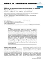
Figure 1. Morphological map of the Aegean Sea and surroundings, the locations of cores
used in this study, and the locations of cores LC21 and T87/2/27 (discussed in text), and
major rivers. Bathymetric contours are at 200 m intervals, and darker tones in the Aegean
Sea indicate greater water depths. NSB = North Skiros Basin, EB = Euboea Basin, MB
= Mikonos Basin, NIB = North Ikaria Basin, SIB = South Ikaria Basin. Core names are
abbreviated: 02 = MAR03-02, 03 = MAR03-03, 25 = MAR03-25, 27 = MAR03-27, 28 =
MAR03-28. Red arrows = surface water circulation from Olson et al. (2006) and Skliris et
al. (2010). Elevation scale in kilometers.

The physical oceanography of the Aegean Sea is
controlled by the regional climate, the freshwater discharge

from major rivers draining southeastern Europe, and
seasonal variations in the Black Sea surface-water outflow
through the Strait of Dardanelles. Previous studies reveal
a general cyclonic water circulation in the Aegean Sea, on
which is superimposed a number of mesoscale cyclonic
and anticyclonic eddies (Casford et al., 2002). A branch
of the westward-flowing Asia Minor Current deviates
toward the north from the eastern Mediterranean basin,
carrying the warm (16–25 °C) and saline (39.2–39.5 psu)
Levantine Surface Water and Levantine Intermediate
Water along the western coast of Turkey. These water
masses occupy the uppermost 400 m of the water column.

The Asia Minor Current reaches the northern Aegean Sea
where it encounters the relatively cool (9–22 °C) and less
saline (22–23 psu) Black Sea Water and forms a strong
thermohaline front. As a result, the water column structure
in the northern and central Aegean Sea comprises a
20–70-m-thick surface veneer consisting of modified
Black Sea Water overlying higher salinity Levantine
Intermediate Water that extends down to 400 m. The water
column below 400 m is occupied by the locally formed
North Aegean Deep Water with uniform temperature (13–
14 °C) and salinity (39.1–39.2 psu; Zervakis et al., 2000,
2004; Velaoras and Lascaratos, 2005). The surface and
intermediate waters follow the general counter-clockwise
circulation of the Aegean Sea, and progressively mix as
they flow southwards along the east coast of Greece.

21



İŞLER et al. / Turkish J Earth Sci
There are several moderate-size rivers that discharge
into the Aegean Sea, including the Meriç, Nestos, Strimon,
Axios, and Aliakmon rivers in the north, and the Gediz
and Büyük and Küçük Menderes rivers in the east (Figure
1). These rivers drain southeastern Europe and western
Turkey with a combined average annual discharge of ~1400
m3 s–1, and an average annual sediment yield of ~229 ×
106 t (Aksu et al., 1995). Most of this sediment is trapped
on the shelves, but considerable quantities bypass the shelf
edge, accounting for high sedimentation rates of 10–30 cm
kyr–1 in deeper basins (e.g., İşler et al., 2008). The Aegean
Sea also receives large quantities of Black Sea surface water
at an average rate of ~400 km3 yr–1 through the Strait of
Dardanelles. Most of this outflow occurs during the late
spring and summer, closely correlating with the maximum
discharge of large European rivers draining into the Black
Sea. However, nearly all the sediments carried by these
rivers are stored in the Black Sea.
2. Materials and methods
Several long piston and gravity cores were collected from
the Aegean Sea during the MAR03 cruise of the RV Koca
Piri Reis using a 12-m-long Benthos piston corer (1000 kg
head weight) triggered by a 3-m-long gravity corer (Figure
1; Table 1). The amount of core penetration was estimated
by the mud smear along the core barrels, and subsequently
compared with the actual core recovery. The gravity cores
were used to determine and quantify potential core-top

loss during the piston coring operation. All cores were
kept upright onboard and during transport to Canada.
Cores were split and described at Memorial University of
Newfoundland. Sediment colour was determined using
the “Rock-Color Chart” published by the Geological
Society of America in 1984. Five key cores were sampled
at 10-cm intervals. Approximately 7-cm3 and 13-cm3
sediment samples were collected for stable-isotopic and
faunal studies, respectively.
Planktonic foraminifera were studied in five cores.
Samples were dried in a 40 °C oven for 48 h, weighed,
transferred to glass beakers, and disaggregated in 100
cm3 of distilled water containing 15 cm3 of 1% Calgon

(Na-hexametaphosphate) and 10 cm3 of 30% hydrogen
peroxide. Next, samples were wet sieved through a 63 µm
sieve, dried in a 40 °C oven, and the >63 µm fractions were
stored in glass vials. Each sample was subsequently drysieved through 150 and 500 µm sieves. The 150–500 µm
fractions were divided into aliquots using a microsplitter
until each subsample contained no less than 300 planktonic
foraminiferal tests. Each aliquot was then transferred to
a cardboard counting slide. All planktonic foraminifera
were identified and counted in each subsample. The
taxa identified in the subsamples were converted into
percentages of the total number of planktonic foraminifera.
Identifications follow the taxonomic descriptions reported
by Parker (1962), Saito et al. (1981), and Hemleben et al.
(1989). The total planktonic foraminiferal abundances in
each sample were calculated as ‘number of specimens per
dry-weight sediment’.

Sea-surface temperature (SST) and sea-surface salinity
(SSS) were calculated from each sample’s planktonic
foraminiferal assemblage using the transfer function
technique developed by Imbrie and Kipp (1971), and the
functional relationships of Thunell (1979). The standard
errors for the summer and winter SST are 1 °C and 1.2
°C, respectively. The SST and SSS values obtained using
the planktonic foraminiferal transfer function compare
well with CTD casts acquired during two field seasons
(Table 2), although the summer SST values from the
transfer function results are slight overestimates. However,
these SST estimates are within the annual range of water
temperatures in the Aegean Sea.
For oxygen isotopic analyses, the planktonic
foraminifera Globigerinoides ruber and the benthic
foraminifera Uvigerina mediterranea were used. For a few
samples, where G. ruber was absent, Globigerina bulloides
was picked instead. For planktonic foraminifera, the
oxygen and carbon isotopic values of both G. ruber and G.
bulloides are plotted using different colours and scales (see
Appendices 1 and 2). There are 30 samples in which both G.
ruber and G. bulloides were analysed: these samples show
a clear and remarkably consistent offset. The oxygen and
carbon isotopic data were replotted (the middle column;

Table 1. Location and water depth of cores used in this study. A = length of piston core, B = length of gravity core, C = amount of core
top loss during coring, D = length of the composite core. Navigation is obtained using a global positioning system.
Core

Latitude


Longitude

A (cm)

B (cm)

C (cm)

D (cm)

MAR03-02

38°03.97ʹN

26°22.30ʹE

776

86

37

813

398

MAR03-03

37°51.72ʹN


25°49.17ʹE

580

50

24

604

720

MAR03-25

37°10.36ʹN

26°26.55ʹE

604

25

25

629

494

MAR03-27


38°18.68ʹN

25°18.97ʹE

952

106

80

1032

651

MAR03-28

39°01.02ʹN

25°01.48ʹE

726

165

100

826

453


22

Water (m)


İŞLER et al. / Turkish J Earth Sci
Table 2. Comparison between the sea surface temperatures and salinities obtained using the planktonic foraminiferal transfer
function and the summer sea surface temperatures and salinities obtained in CTD casts during cruises in 1991 (Aksu et al.,
1995b) and 2003 (Institute of Marine Sciences and Technology, Dokuz Eylül University, unpublished data).
2003 (°C)

2003 (psu)

1991 (°C)

1991 (psu)

SSTw (°C)

SSTw (°C)

MAR03-02

23.44

39.79

24.55


39.43

18.99

27.17

MAR03-03

23.92

39.50

24.55

39.42

18.99

27.17

MAR03-25

21.55

39.70

23.56

39.35


18.08

25.75

MAR03-27

22.50

39.57

23.44

39.23

18.99

27.33

MAR03-28

23.43

39.28

24.53

39.15

19.38


27.61

Appendices 1 and 2) by shifting the G. bulloides curve
by ~1 permil, but clearly showing a scale for G. bulloides
for clarity. Then a pseudocomposite section was created,
but showing the isotopic values for both G. ruber and G.
bulloides with separate horizontal scales and different
colours. This pseudocomposite plot is carried forward
into figures in the main text that require the oxygen and
carbon isotopic records of cores M03-27 and M03-28.
The reader is reminded that (with separate isotope scales
and colours) two species were used in these two cores. In
each sample 15–20 G. ruber and 4–6 U. mediterranea (or
15–20 G. bulloides) were hand-picked from the >150 µm
fractions, cleaned in distilled water, and dried in an oven
at 50 °C. The foraminiferal samples were then placed in
12 mL autoinjector reaction vessels. The reaction vessels
were covered with Exetainer screw caps with pierceable
septa, and were placed in a heated sample holder held at
70 °C. Using a GC Pal autoinjector, the vials were flushed
with ultrahigh purity He for 5 min using a doubleholed needle connected by tubing to the He gas source.
Sample vials were then manually injected with 0.1 mL of
100% H3PO4 using a syringe and needle. A minimum of
1 h was allowed for carbonate samples to react with the
phosphoric acid. The samples were analysed using a triple
collector Thermo Electron Delta V Plus isotope ratio mass
spectrometer. Reference gases were prepared from three
different standards of known isotopic composition using
the same methods employed for the unknown samples,
and were used to calibrate each run. The δ18O and δ13C

values are reported with respect to the Pee Dee Belemnite
(PDB) standard.
For trace-element measurements on foraminifera, 10–
15 tests were placed in a small vial with distilled water and
cleaned using an ultrasonic cleaner for 30 s, then rinsed,
and dried in an oven at 40 °C. Five specimens of G. ruber
from each sample were mounted on 2.5 × 5 cm glass slides
with double-sided sticky tape, with the aperture facing
upwards. Mg and Ca concentrations in the carbonate
foraminiferal tests were obtained using a Finnigan

ELEMENT XR, a high-resolution double-focussing
magnetic-sector inductively coupled plasma mass
spectrometer (HRICPMS), and a GEOLAS excimer laser
(λ = 193 nm) at Memorial University of Newfoundland.
The laser was focussed on the sample and fired at 5 Hz
repetition rate using an energy density of 5 J/cm2 and 59
µ laser spot diameter. Between 5 and 6 pits were laserablated for each G. ruber specimen, with no more than 2
pits on a single chamber. Thus, an average of 30 ablations
(5 specimens × 6 ablations) was carried out in each sample.
The results are expressed as Mg/Ca (mmol/mol) ratio.
Standard deviation of the Mg content in G. ruber tests is
calculated to be approximately 0.02 µg based on replicate
measurements on a number of randomly selected samples
at several depths from cores MAR03-28 and MAR03-02.
Mg/Ca temperature calculations were performed using the
equation Mg/Ca = 0.340.102 × T from Anand et al. (2003).
This equation is preferred because it was constructed for G.
ruber (white) (250–350 µm), which is the same species and
size range used in this study. Due to the logarithmic nature

of the Mg/Ca temperature equation, cooler temperatures
(low Mg content) are associated with larger error bars. The
standard errors for cores MAR03-28 and MAR03-02 are,
respectively, 1.7–6.8 °C and 1.4–5 °C, with an average of 3
°C and 2.5 °C.
Stacked planktonic and benthic oxygen and carbon
isotope curves were constructed by averaging the isotopic
values in cores MAR03-02, MAR03-03, MAR03-25,
MAR03-27, and MAR03-28. The 0–110 ka portions of
the stacked planktonic curves were constructed using the
average isotopic values of only G. ruber in cores MAR03-02,
MAR03-28, and MAR03-27. The sections corresponding
to 110–130 ka are the δ18O and δ13C curves from core
MAR03-28. The 0-110 ka portions of the stacked benthic
isotope curves were constructed using the average isotopic
values in cores MAR03-02, MAR03-03, MAR03-25, and
MAR03-28. The sections pertaining to 110–130 ka are
the average of the isotopic values in cores MAR03-03 and
MAR03-28.

23


İŞLER et al. / Turkish J Earth Sci
3. Results
3.1. Lithostratigraphy
On the basis of visual core descriptions, organic carbon
content, and colour, four sapropel and five nonsapropel
units are identified and labeled as ‘A’ through ‘I’ from top
to bottom (Figure 2). The correlation of the units among

the five cores (Figure 3) was accomplished by matching
peaks of oxygen isotopic curves together with the
stratigraphic positions of geochemically fingerprinted ash
layers (Aksu et al., 2008). Throughout the cores, sapropel
units are distinguished by their darker colors and higher
organic carbon contents. However, rather than a fixed
quantitative threshold (e.g., >0.5%, >1%, or >2% TOC
content), an organic carbon content twice (or more) that
of the underlying and overlying units was used to classify
a lithostratigraphic unit as a sapropel. Using this criterion,
sediments with 1.0%–12.65% TOC content are described
in this paper as sapropels. Most sediments consist of clay/
silt mixtures that are slightly to moderately burrowed. The
coarse fraction is mainly foraminifera, pteropods, bivalve,
and gastropod shells, and variable amounts of volcanic
ash. Sediment accumulation is inferred to have occurred
through hemipelagic rain due to paucity of terrigenous
sand-sized material, lack of evidence for resedimentation
as normally graded beds, and ubiquitous bioturbation.
Nonsapropel units A, C, E, G, and I are composed of
burrow-mottled foraminifera-bearing calcareous clayey
mud. The units are predominantly yellowish to dark
yellowish brown (10YR5/4, 10YR4/2) and various shades of
gray (i.e. yellowish, light, and dark; 5Y5/2, 5Y6/1, 5GY6/1).
The TOC content is 0.4%–0.7% (average 0.5%) with higher
organic carbon contents in unit G reaching 0.9% (Figure
2). Unit A contains an ash layer largely disseminated in
fine mud. The ash is widespread throughout the Aegean
Sea and has been identified by geochemical fingerprinting
as the Z2 tephra from the Minoan eruption of Santorini

Island (Aksu et al., 2008).
Unit C contains three tephra layers which are described
in detail by Aksu et al. (2008), and identified by those
authors using geochemical fingerprinting. From top to
bottom they are the Y2 tephra (the Cape Riva eruption
on the Island of Santorini also known as the Akrotiri
eruption), the Y5 tephra (Campanian Ignimbrite eruption
of the Phlegran Fields of the Italian Volcanic Province),
and the Nisyros tephra (Nisyros eruptions on the Island of
Nisyros). High numbers of glass shards make the tephra
layers discernible with sharp tops and bases in most of
the cores; however, some are disseminated in fine mud.
For example, Unit E contains an ash layer, disseminated
in mud in cores MAR03-25 and MAR03-02, which is
correlated with the X1 tephra, most likely derived from the
Aeolian Islands, Italy (Aksu et al., 2008).

24

Sapropel units B, D, F, and H are distinguished from
overlying/underlying units by their darker olive gray
colour (5Y4/1, 5Y3/2, 5Y4/2, 5Y5/2, 5Y2/2, 5Y2/1).
They are composed of sharp-based colour-banded clayey
mud overprinted by sharp-walled branching millimetrediameter burrows identified as Chondrites. The organic
carbon contents range from 1% to 12.65%.
3.2. Age models
The chronostratigraphy of the cores was established using
a number of age control points that permit a depth-to-age
conversion with the assumption that the sedimentation
rate was constant between dated levels. The age control

points consist of well constrained top/bottom ages of unit
B (sapropel S1); tephra layers Z2, Y2, and Y5; and control
points determined by curve matching of the oxygen isotope
curves for each core with the global oxygen isotope curve
of Lisiecki and Raymo (2005). The Nisyros ash (Figure
3) was not used because the age proposed by Aksu et al.
(2008) for this tephra is now in question (Margari et al.,
2007) and it is likely older than Aksu et al. (2008) reported,
perhaps 54–58 ka rather than 42–44 ka (V. Margari and
D. Pyle, pers. comm. 2011). Unit B is correlated with the
most recent sapropel S1 due to its consistent stratigraphic
position throughout the cores, situated between the ash
layers Z2 and Y2, and its occurrence within MIS 1. Its top/
bottom ages (6600 and 9900 14C yr BP, respectively; Table
3) are well constrained by other researchers; calibrated
dates based on these 14C ages and a reservoir age of 557
yr (Facorellis et al., 1998) are used as age control points.
The oldest sediment recovered in the cores (unit I) was
deposited ~130 ka at the transition from MIS 6 to MIS 5
(Table 3).
The interpolated basal ages of organic-rich Units D, F,
and H are 83.2–80.4 ka, 106.4–105.8 ka, and 128.6–128.4
ka, respectively. These calculated ages coincide with the
substages of MIS 5 and are in good agreement with the
previously published ages of sapropels S3, S4, and S5
developed during marine isotopic stages 5a, 5c, and 5e in
the eastern Mediterranean Sea (Rossignol-Strick, 1985;
Emeis et al., 2003).
The mean sedimentation rates for cores MAR03-28,
MAR03-03, MAR03-02, MAR03-25, and MAR03-27 are

6.4 cm/ka, 4.7 cm/ka, 9.5 cm/ka, 6.0 cm/ka, and 11.5 cm/
ka, respectively (Table 3). Considering the 10-cm sampling
interval, calculated accumulation rates imply a temporal
sample-to-sample resolution for these cores of 1560 yr,
2125 yr, 1050 yr, 1665 yr, and 870 yr, respectively.
3.3. Planktonic foraminifera
All samples examined for foraminifera include variable
amounts of aragonitic pteropods, which suggest that the
foraminifera in the Aegean Sea cores sustained little to no
dissolution and that the observed fauna in the cores likely


Depth (m)

10

9

8

7

6

5

4

3


2

1

S3

Nis

Y5

Y2

S1

Z2

E

D

C

B

A

MAR03-27

0


1

2

TOC (%)

5

3 4

1

3

0

18

2

1

G. ruber

G. bulloides

2

G. bulloides
δ O (‰ PDB)


4

3

0

-1

S5

S4

S3

Nis

Z2
S1
Y2
Y5

D
E
F
G
H
I

C


A
B

F
G
H
I

E

D

C

A
B

MAR03-03

S5

S4

S3

Nis

Y5


Y2

Z2
S1

δ18 O (‰ PDB) MAR03-28
G. ruber

0

0

2

8.97

9.41

1

9.62

3

2

3

0


4

3

-1

2

2

1

1

0

G. ruber

G. bulloides

1

U. mediterranea
G. bulloides

4

benthic

δ18 O (‰ PDB)

G. ruber

δ18 O (‰ PDB)
U. mediterranea

35

9.35

2

TOC (%)

5

3 4

5.61 12.65

1

TOC (%)

F
G

D
E

S3

X1
S4

Y5
Nis

Y2

Z2
S1

D
E
F
G

C

A
B

MAR03-25

X1

Nis

Y5
C


B

S1
Y2

A

Z2

MAR03-02

0

0

1

2

2

2
0

4

3

3


2

2

1

1

U. mediterranea
δ18 O (‰ PDB)

4

1

planktonic

benthic

3

0

-1

δ18 O (‰ PDB)
G. ruber

δ18 O (‰ PDB)
U. mediterranea

3 5

5

34

3.15

TOC (%)

1

TOC (%)

İŞLER et al. / Turkish J Earth Sci

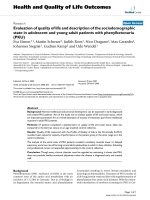
Figure 2. Downcore plots showing the lithostratigraphic units (A through I), total organic carbon (TOC) contents
and the variations in oxygen isotope values (δ18O) in the Aegean Sea cores. Red and blue lines are the δ18O values
in planktonic foraminifera G. ruber and G. bulloides, respectively, aquamarine lines are the δ18O values in benthic
foraminifera U. mediterranea. MIS = marine isotopic stages. Black fills = sapropels, red fills = volcanic ash layers (from
Aksu et al., 2008). Core locations are shown in Figure 1.

25


İŞLER et al. / Turkish J Earth Sci

S3

S4


S5

82,800

106,400

----

MAR03-02

Onset
End

76,600

94,400

----

MAR03-03

Onset

83,200

105,800

128,600


End

72,600

100,600

123,600

MAR03-25

Onset

81,600

105,600

----

End

76,800

97,800

----

MAR03-27

Onset


80,400

----

----

End

74,000

----

----

Onset

80,600

105,800

128,400

End

70,800

96,200

121,000


MAR03-28

represent the surface water assemblages near each core site
at the time of deposition. In basins where the foraminiferal
lysocline is deep and bottom waters are not corrosive, the
living planktonic foraminiferal assemblages in surface
waters are well represented in the bottom sediments (e.g.,
Schiebel et al., 2004, Retaileau et al., 2012).

N. Ikaria
Basin
MAR03-02

N. Skiros
Basin
MAR03-28
0

(453 m)

1
2

(398 m)

Z2

S1

S1


Y2

Y2

Depth (m)

Y5
Nis

5
6
7
8
9

10

?

S3
X1
S4
S5

Euboea
Basin
MAR03-27

(720 m)


Z2

3
4

Mikonos
Basin
MAR03-03

(494 m)

Z2
S1

sapropels
tephra
δ18O
stages
layers
Z2

S1

Y2

1

0


2

Y5

Y2
Y2

Nis

S2

Y5
S3
Y5

Nis

3

S4
Nis

50

4

5

100


X1

Nis
?

S5
S3

S4
S5

S. Ikaria
Basin
MAR03-25

(651 m)

Z2
S1

Y5

S3
X1

3.3.1. Downcore distribution of planktonic foraminiferal
ecozones
Seventeen planktonic foraminiferal species were
identified. The dominant species that constitute >85% of
the total assemblage are N. pachyderma dextral (hereafter

denoted by d), G. bulloides, G. ruber (white), Turborotalita
quinqueloba, G. inflata, Globigerinita glutinata, G. scitula,
Orbulina universa, and N. dutertrei. The remaining eight
species (Globigerinella aequilateralis, Globigerinoides
sacculifer, G. ruber (pink), Globigerinella calida,
Globorotalia crassaformis, Globigerinoides rubescens,
Globigerinoides tenellus, and N. pachyderma (sinistral;
hereafter denoted by s)) display sporadic appearances
not exceeding 5% of the total fauna. Tropical taxa (i.e. G.
aequilateralis, G. sacculifer, G. ruber (pink), G. calida, G.
crassaformis, G. rubescens, and G. tenellus) occur together
and are only present in low abundances; they are plotted
together as the parameter ‘warm’.
The planktonic foraminiferal data matrix was used to
perform a ‘mean-within cluster sum of squares’ cluster
analysis, CONISS (CONstrained Incremental Sums of
Squares; Grimm, 1987). The final clusters were delineated
by drawing a straight line at the value 0.04 on the distance/

Age (ka)

Table 3. Calculated ages of sapropels S3, S4, and S5.

Nis

X1

S3

S3

X1

W1
W2
W3

S4

V1
V3

6

150

S6
S7

7

200

Figure 3. Correlation of ash layers (red) and lithostratigraphic units across the Aegean Sea cores. Ash layers Z2, Y2, Y5, Nis, X1 (red
fills) are from Aksu et al. (2008). Sapropels are shown as black fills with S1, S3, S4, and S5 designations. Global oxygen isotopic stage
boundaries are from Lisiecki and Raymo (2005). Core locations are shown in Figure 1.

26


İŞLER et al. / Turkish J Earth Sci

similarity measure of each dendrogram. Species that are
associated (i.e. that cluster) in the distance/similarity range
0.00–0.04 are recognized as ‘planktonic foraminiferal
ecozones’, hereafter referred to as ‘ecozones’ I though IV.
Ecozone IV is further subdivided into six subecozones
(Figures 4–8). In this study, the ecozones are arranged
stratigraphically, through time, without downcore
repetition.
The downcore variations in the proportions of
individual planktonic foraminifera generally show
distinctive distribution patterns broadly correlated with
the ecozones identified using the cluster analysis results,
suggesting that the large-scale climatic and oceanographic
conditions across the Aegean Sea during the Late
Quaternary are faithfully recorded by the planktonic
foraminiferal data (e.g., Schiebel et al., 2004).
Ecozone I (0–13 ka) is characterized by high
abundances of G. ruber and G. bulloides (>85% of the
total foraminiferal assemblage), the consistent presence
of the tropical species, and episodic appearances of N.
pachyderma(s), G. inflata, and O. universa (Figures 4–8).
G. ruber exhibits a higher amplitude variation, particularly
within the upper half of the ecozone.
Ecozone II (~40–13 ka) is characterized by the
dominance of N. pachyderma (d), low percentages of G.
ruber and G. bulloides, and the absence of G. inflata. N.
pachyderma (d) generally increases upward; for example,
from 43% to 81% in core MAR03-28 and from 27% to
51% in core MAR03-25 (Figures 4–8). G. ruber shows
low percentages (<10%) and, particularly in the most

northerly core MAR03-28, abundances do not exceed
5% in the middle portion of the ecozone. T. quinqueloba
is consistently present in all cores, ranging from 1% to
~30%. G. glutinata ranges between 1% and 22%, whereas
G. scitula, N. pachyderma (s), and N. dutertrei are generally
<10%.
Ecozone III (~40–60 ka) is characterized by the
continuous presence of G. inflata and lower abundance
variations of N. pachyderma (d) relative to Ecozone II
(Figures 4–8). G. ruber and G. bulloides exhibit moderate
frequency and high amplitude variations throughout
the cores, ranging generally between 10% and 40%. T.
quinqueloba shows a negative excursion similar to N.
pachyderma (d), attaining high percentages of 20%–25% at
the base and top of the ecozone and decreasing to 4%–11%
in the middle. Ecozone III is marked at its base by a mostly
sharp to locally gradual downward disappearance of G.
inflata (Figures 4–8).
Ecozone IV (>60 ka) is characterized by large
amplitude variations in the abundances of N. pachyderma
(d), G. ruber, and G. bulloides and episodic appearances
of N. dutertrei (Figures 4–8). These variations are used to
subdivide the ecozone into six subecozones, IVa–IVf.

Subecozone IVa is characterized by a dominance of
N. pachyderma (d), downward increase in N. dutertrei,
and consistent upward increase in G. ruber (Figures
4–8). G. bulloides generally varies from 12% to 35% and
T. quinqueloba and G. inflata generally show consistent
abundances ranging between ~5% and 30% and between

3% and 38%, respectively.
Subecozone IVb is characterized by a dominance
of G. ruber (38%–58%) and G. bulloides (13%–25%),
near disappearance of N. dutertrei, and general upward
increasing trend of G. inflata (~6%–21%; Figures 4–8).
N. pachyderma (d) displays large amplitude negative
inflections with values ranging between 33% and 65%.
Subecozone IVc is characterized by high abundances of
N. pachyderma (d) (~30%–75%) and very low abundances
of G. ruber (~4%), G. bulloides (~7%), and N. dutertrei
(8%) (Figures 4–8). Generally, the maximum abundances
of N. dutertrei coincide with the minimum abundances of
G. inflata.
Subecozone IVd is characterized by low N. pachyderma
(d) percentages, notably increased abundances of G. ruber
and G. bulloides, and the disappearance of T. quinqueloba
and N. dutertrei (Figures 4–8).
Subecozone IVe coincides with high abundances of N.
pachyderma (d) (65%–70% in only cores MAR03-03 and
MAR03-28; Figures 4 and 7). G. ruber and G. bulloides
exhibit negative excursions with abundances of 20%–40%.
N. dutertrei and O. universa are consistently present across
the subecozone, generally showing abundances of 6%–9%
(Figures 4 and 7).
Subecozone IVf covers the lowermost portions of
cores MAR03-03 and MAR03-28 (Figures 4 and 7). G.
bulloides ranges between ~20% and 40%. N. pachyderma
(d) ranges between >20% and <60%.
3.4. Oxygen isotopes
The age-converted stacked δ18O curves for planktonic and

benthic foraminifera illustrate that there are consistent
variations in the oxygen isotopic composition of the
Aegean Sea water masses since 130 ka. Moderate to large
amplitude excursions correspond to glacial and interglacial
stages (Figure 9). Abrupt depletions in the δ18O values
characterize the upper segments of all cores with changes
of as much as 4‰ at the most recent glacial–interglacial
transition (i.e. marine isotopic stage MIS 2/1 boundary;
Figure 9). Planktonic foraminiferal δ18O values are notably
heavier during glacial periods (i.e. 2.8‰–3.2‰ in MIS 2
and MIS 4), suggesting cooler and possibly more saline
conditions. Similar to the trends observed in global oxygen
isotopic data (e.g., Lisiecki and Raymo, 2005) downcore
variations in oxygen isotope values in the Aegean Sea
cores show that the interglacial–glacial transitions are
more gradual than the glacial–interglacial transitions. The
depleted δ18O values during MIS 1 and MIS 5 show clear

27


0

20 10 0

20 10 0

20 0

20


Ecozones
10

20

08

0

0.

40 60

T.
qu
in
qu
N.
pa elob
a
c
N. hyd
du er
O. tert ma
un re (s)
i
G. iver
sc sa
G. itul

in a
fla
ta
W
ar
m

G.
bu
llo
id
es
20

40 60 0

06

20

0.

10 0

0.

80

02


40 60

04

20

0.

0

CONISS
0.

0

G.
g
G. lutin
ru at
be a
r(w
)

N.
pa
ch
yd
er
m


MAR03-28

a(
d)

İŞLER et al. / Turkish J Earth Sci

I

20
II

Age (ka)

40
III

60
IVa

80
IVb

100

IVc
IVd

120


IVe
IVf

Hemipelagic muds

Sapropel/sapropelic muds

Discrete tephra beds

0

20

40

60

80

20

40 60 0

20

N.

pa

nq

ui
T.
q

40 60 0

Ecozones

lo
N. ch ba
y
du d
e
O. tert rma
un rei (s
)
iv
G. ersa
s
G. citu
in la
fla
ta
W
ar
m

ue

es

id
llo
bu
G.

ru

G.
20 0

CONISS

20

10 0

20

20 10 0

20 0

20

0.
02
0.
04
0.
06

0.
08
0.
10
0.
12

0

G.

N.

gl

pa

ut

in

ch
yd
e

at
be a
r(w
)


rm

MAR03-27

a(
d)

Figure 4. Downcore assemblage distributions of planktonic foraminifera in core MAR03-28. The right column shows the results of
cluster analysis and the resulting ecozones. Core location is shown in Figure 1.

I

20

Age (ka)

II

40
III

60
IVa

80

IVb

Hemipelagic muds


Sapropel/sapropelic muds

Discrete tephra beds

Figure 5. Downcore assemblage distributions of planktonic foraminifera in core MAR03-02. The right column shows the results of
cluster analysis and the resulting ecozones. Core location is shown in Figure 1.

28


0

20

40 60

80 0

20 0

20

T.
q

20

40 60 0

20


0

20

0

20

40 0

20

Ecozones

ui
nq

ul
lo
id
es
G.
b

40 60 0

CONISS

0.

02
0.
04
0.
06
0.
08
0.
10
0.
12

0

G.
gl
ut
G. inat
a
ru
be
r(w
)

N.
p

ac
hy
de

rm
a(
d)

MAR03-02

ue
lo
N.
ba
pa
N. ch
du yde
t e rm
O. rtre a(s
i
)
u
G. nive
s c rs a
i
G. tula
in
fla
ta
W
ar
m

İŞLER et al. / Turkish J Earth Sci


I

20
II

Age (ka)

40
III

60
IVa

80
IVb

100

IVc
IVd

Hemipelagic muds

Sapropel/sapropelic muds

Discrete tephra beds

0


20

ui
40 60 0

20

10 0

20 0

20 0

20

10 0

20

Ecozones

nq

id
llo
bu

40 60

pa uel

N. chy oba
du de
te rm
O. rtre a(
i s)
un
ive
G.
r
sc sa
itu
la
G.
in
W flat
ar a
m

es

)
r(w

be
20

N.

20 0


T.
q

80 0

ru

gl
40 60

G.

20

G.

0

CONISS

0.
02
0.
04
0.
06
0.
08
0.
10

0.
12

0

G.

N.

pa

ut

in

at

ch
yd
e

a

rm

MAR03-03

a(
d)


Figure 6. Downcore assemblage distributions of planktonic foraminifera in core MAR03-03. The right column shows the results of
cluster analysis and the resulting ecozones. Core location is shown in Figure 1.

I

20
II

Age (ka)

40
III

60
IVa

80
IVb

100

IVc
IVd

120

IVe
IVf

Hemipelagic muds


Sapropel/sapropelic muds

Discrete tephra beds

Figure 7. Downcore assemblage distributions of planktonic foraminifera in core MAR03-03. The right column shows the results of
cluster analysis and the resulting ecozones. Core location is shown in Figure 1.

29


0

20

40 60

20

40 60 0

20

10 0

20 0

20

10 0


20 0

20

Ecozones

T.
qu
i
N. nqu
pa elo
c
N. hyd ba
du er
m
t
O. ertr a (
un ei s)
i
G. vers
sc a
i
G. tula
in
fl
W ata
ar
m


id
es
lo
0

0.
08

20

G.
bu
l

at
a
G.
ru
be
r(w
)

tin
lu

40 60 0

0.
06


20

0.
02

0

CONISS
0.
04

0

G.
g

N.
pa
ch
yd
er
m

MAR03-25

a(
d)

İŞLER et al. / Turkish J Earth Sci


I

20
II

Age (ka)

40
III

60
IVa

80
IVb

100

IVc
IVd

Hemipelagic muds

Sapropel/sapropelic muds

Discrete tephra beds

Figure 8. Downcore assemblage distributions of planktonic foraminifera in core MAR03-25. The right column shows the results of
cluster analysis and the resulting ecozones. Core location is shown in Figure 1.


association with times of sapropel deposition. The data
show that depletions are strongest during and immediately
following the accumulation of sapropels S1 and S5, ranging
from 0.6‰ to 0.9‰ in U. mediterranea and from 0.3‰ to
–0.6‰ in G. ruber and G. bulloides. In sapropels S3 and S4,
δ18O values show similar yet modest variations changing
on average by between 1.4‰ and 1.8‰ relative to adjacent
units. In cores MAR03-28 and MAR03-02, the magnitudes
of the depletions and enrichments in the planktonic and
benthic δ18O values are similar to one another (Figure 9).
3.5. Carbon isotopes
Carbon isotope values obtained from planktonic and
benthic foraminifera generally range between 0.0‰ and
1.5‰ with conspicuous depletions (–0.5‰ and –1.0‰)
in the uppermost parts of cores MAR03-25 and MAR0302, coinciding with sapropel S1 (Figure 10). Consecutive
and large amplitude excursions of as much as 1.0‰ are
recognized in the lower half of the cores (encompassing
MIS 5), where sapropel layers S3, S4, and S5 generally
correlate with the δ13C depletions.
3.6. Sea surface temperature (SST) and sea surface
salinity (SSS)
Based on transfer-function calculations, high amplitude
temperature and salinity variations of ~8–12 °C and 1.5
psu occurred during MIS 5 and the transition from MIS 2
to MIS 1 (Figure 11). Fluctuations during MIS 5 are notably

30

larger in cores MAR03-28 and MAR03-03 than those in
cores MAR03-25 and MAR03-02. Within the upper half

of sapropel S5 in cores MAR03-28 and MAR03-03, SST
and SSS values show a progressive upward increase into
the overlying nonsapropel unit G, changing from 14 °C to
23 °C and from 36.7 psu to 38.3 psu. In core MAR03-28,
SST and SSS estimates are around 16 °C and 37.3 psu at the
top and bottom of sapropel S5 and are lower (13.6 °C and
35.2 psu) immediately above the middle of the sapropel at
around 125 ka (Figure 11).
Toward and well into the time of accumulation of
sapropel S4, temperature and salinity decreased at all
core sites and minima were attained mainly close to
the sapropel top (except in core MAR03-02). At core
sites MAR03-28 (most northerly) and MAR03-03, the
magnitude of these drops was as much as 10 °C and 1.8
psu. During the deposition of sapropel S4, surface waters
were warmer and more saline at southernmost core site
MAR03-25 than at other sites, changing between 21 °C and
37.9 psu at the base of S4 to 19 °C and 36.7 psu at its top.
Minimum temperature and salinity values of 11.8 °C and
36.5 psu were calculated within the upper half of sapropel
S4 at the most northerly core site MAR03-28, becoming
16–17 °C and 37.6 psu at the bottom and top of S4 (Figure
11). In core MAR03-02, SST shows a continuous upward
increase from 17 °C to 21.8 °C across S4 with relatively


İŞLER et al. / Turkish J Earth Sci
MAR03-28
0


MIS

20

Age (ka )

40

4

1

Z2
S1

2

Y2
Y5

3

3

δ18 O (‰ PDB)
G. ruber
2

1


0

G. bulloides
C

S3

5

S4

G. ruber

S5
6

140

5

4

H
I

benthic
5

δ18 O (‰ PDB)
planktonic

3

2

1

4

0

-1

20

stacked
planktonic

Age (ka)

40

3

2

S4

1

D


S3

E

X1

F
G

S4

1
2

Y2
Y5

100

S3

5c
5d

120

D
E


0

-1

benthic

F
6

5

δ18 O (‰ PDB)
G. ruber
3

2

1

MAR03-25
Z2
S1

G. bulloides

Y5

G. ruber
D
E


4

3

2

G. bulloides
δ18 O (‰ PDB)

2

4

3

2

1

1

A
B

Y2

C

5


3

δ18 O (‰ PDB)
U. mediterranea

5

0

A
B

4

U. mediterranea
δ18 O (‰ PDB)

H
I

4

5b

stacked
benthic

1


C

G

MAR03-27
Z2
S1

5a

2

A
B

Nis

benthic

4

80

140

C

Nis

60


3

δ18 O (‰ PDB)
G. ruber

planktonic

MIS

3

4
Z2
S1

Y5

S5

U. mediterranea
G. bulloides

1

Y5

G

120


0

F

2

Y2

S3

D

3

Y2

E
100

4

MAR03-02

A
B

Nis

4


80

δ18 O (‰ PDB)
U. mediterranea

5

-1
Z2
S1

A
B

Nis

60

MAR03-03

C

Nis

benthic

S3
X1


D
E

S4

F
G

1

5e
6

5

4

3

2

1

0

U. mediterranea
δ18 O (‰ PDB)

-1


Figure 9. Generalized downcore variations of oxygen isotopic compositions in planktonic foraminifera G. ruber (red) and G. bulloides
(blue) and benthic foraminifera U. mediterranea in the Aegean Sea during the last ca. 130 ka. Graph on the lower left is the stacked
planktonic and benthic oxygen isotopic compositions (red and aquamarine shaded envelopes, respectively). Stacking is achieved by
averaging the age-converted benthic and planktonic oxygen isotopic values in cores MAR03-02, MAR03-03, MAR03-25, MAR03-27,
and MAR03-28. Heavy aquamarine (benthic) and red (planktonic) lines are the averaged values. Core locations are shown in Figure 1.

constant surface salinity (~37 psu). Successive SST and
SSS increases continued above S4 until 86 ka at core site
MAR03-25 and until around 91 ka at the remaining four
core sites, reaching temperatures and salinities ranging
mainly between 21.5 and 22.5 °C and 38 and 38.6 psu.
Toward the onset of sapropel S3, SST and SSS show
a persistent drop until around 82 ka, reaching minimum
values of 18–18.5 °C and 37.3–37.1 psu at core sites

MAR03-25 and MAR03-02 and 12–14 °C and 36.4–36.1
psu in cores MAR03-03 and MAR03-28 (Figure 11).
The SST and SSS values exhibit small variations during
the deposition of sapropel S3, ranging from 10 °C to
13 °C and from 36.4 psu to 37.1 psu at northerly core
sites MAR03-28 and MAR03-27 and from 16 °C to 18
°C and from 36.7 psu to 37.3 psu at core sites MAR0325, MAR03-03, and MAR03-02. Until 46 ka, SST and

31


İŞLER et al. / Turkish J Earth Sci

0


MIS

20
40
Age (ka)

δ13 C (‰ PDB)
MAR03-28 G. ruber U. mediterranea
0

1

Z2
S1

2

Y2
Y5

3

G. ruber

S3

benthic

5


S4

S4

G

120

S5
6

140

H
I

S5
-2

δ13 C (‰ PDB)
G. ruber

-2

-1

0

-1


40
Age (ka)

Z2
S1

Y5

C

D

S3

E

X1
benthic

F
G

2

Y2

3

Y5


stacked
benthic

5c

stacked
planktonic

120

F
0

1

U. mediterranea
δ13 C (‰ PDB)
δ13 C (‰ PDB)
G. ruber
1

2

δ18 O (‰ PDB)
MAR03-25 U. mediterranea
0

Z2
S1


G. ruber

2

A
B

Y2
Y5

C

1

2

C

benthic

Nis

G. bulloides
S3

5b

100

S4


A
B

4
5a

planktonic

D
E

H
I

Nis

60

2

benthic

G

0

1

C


Nis

MAR03-27
Z2
S1

1

A
B

Y2

MIS

1

20

140

0

G. bulloides
δ C (‰ PDB)
13

δ13 C (‰ PDB)
G. ruber


0

2

A
B

Nis

G. bulloides

F

1

MAR03-02

Y2

S3

D
E

100

0

Y5


C

4

80

80

2

Z2
S1

Nis

60

0

1

A
B

δ13 C (‰ PDB)
U. mediterranea

MAR03-03


5d

D
E
-2

-1

S3
X1

D
E

S4

F
G

0

G. bulloides
δ13 C (‰ PDB)

5e
6

0

1


2

U. mediterranea
δ13 C (‰ PDB)

3

Figure 10. Generalized downcore variations of carbon isotopic compositions in planktonic foraminifera G. ruber (red) and G. bulloides
(blue) and benthic foraminifera U. mediterranea in the Aegean Sea during the last ca. 130 ka. Graph on the lower left is the stacked
planktonic and benthic carbon isotopic compositions (red and aquamarine shaded envelopes, respectively). Stacking is achieved by
averaging the age-converted benthic and planktonic carbon isotopic values in cores MAR03-02, MAR03-03, MAR03-25, MAR03-27,
and MAR03-28. Heavy aquamarine (benthic) and red (planktonic) lines are the averaged values. Core locations are shown in Figure 1.

SSS gradually increased and generally show 2–3 °C and
1 psu variations, ranging from 11.5 to 13.5 °C and from
36.5 to 37.2 psu at the most northerly core site MAR0328 and from 18–20.2 °C and 37–38.1 psu to 19.2–22 °C
and 37.2–38.2 psu at more southerly sites MAR03-02 and
MAR03-25, respectively (Figure 11). In core MAR03-27,
relatively extended periods of temperature and salinity
increases are observed until 36 ka. This relatively warm
interval is followed by a continuous drop in surface water

32

temperatures and salinities, indicating the gradual change
from interglacial to glacial conditions associated with the
transition from MIS 3 to MIS 2. At core sites MAR0302, MAR03-03, and MAR03-28, glacial conditions were
attained rather more rapidly (at ~39 ka) than at core sites
MAR03-27 and MAR03-25. The former three core sites

show 4–8 °C and 0.4–1.0 psu drops attaining minimum
temperatures of 11–12 °C at core sites MAR03-03 and
MAR03-02 and 8–10 °C at the most northern core site


İŞLER et al. / Turkish J Earth Sci
MAR03-28
0
20

Age (ka)

40
60

MIS
1

Z2
S1

2

Y2

3

SSS(‰)

SST (°C)


Y5

Z2
S1

A
B

Y5

C

Nis
S3

5

S3

D

F

S4

G

120
140


S4

S5
6

SSTw

H
I

S5

SST (°C)
0
20

Age (ka)

40
60
80

MIS

8 12 16 20 24 28

stacked
SSTs


140

Y5

S3

SSS(‰)
37 38 39

A
B

C

Nis
D

S3

E

X1

F
G

S4

D
E

F
G

H
I

A
B

SST (°C)

SSS(‰)

MAR03-25

SST (°C)

SSS(‰)

8 12 16 20 24 28 36 37 38

37 38 39
Z2
S1

A
B

Y2
C


Y5

C

Nis

4

D
E

5c

5e

Y5

C

Nis

5d
120

stacked
SSS

SST (°C)
8 12 16 20 24 28


Z2
S1

4 8 12 16 20 24 28

Y2

MAR03-02

Y2

MAR03-27

2

5a

37 38

A
B

38
Z2
S1

5b
100


SSS(‰)
37

1

3

SSS(‰)

Nis

E
100

SST (°C)
8 12 16 20 24 28

Y2

SSTs

4

80

MAR03-03

4 8 12 16 20 24 28 36 37 38 39

stacked

SSTw

S3
X1

D
E

S4

F
G

6

Figure 11. Sea surface temperature (SST) and sea surface salinity (SSS) variations of five cores. Horizontal grey bars highlight the
sapropel intervals. MIS = marine isotopic stages. Black fills = sapropels, red fills = volcanic ash layers (from Aksu et al., 2008). Core
locations are shown in Figure 1.

MAR03-28 (Figure 11). These glacial temperature and
salinity values were maintained until 18 ka. Between
18 ka and core tops (Recent), continuous and very high
amplitude temperature and salinity increases are observed
at all core sites, associated with the transition from MIS
2 to MIS 1. The SST values show 1–2 °C temperature
decreases immediately below the most recent sapropel S1.
Cooler and less saline surface waters lingered during the
deposition of sapropel S1 and then the sea surface warmed
up to its previous state following the cessation of sapropel
formation. The SST values continued to rise toward the

core tops, becoming ~2–3 °C warmer since 5 ka (Figure
11).
3.7. SST from Mg/Ca ratios
It has been argued that SST values in geographically
confined seas, such as the Aegean Sea, cannot be reliably
estimated because of the high amplitude fluctuations in
temperature, salinity, and productivity in such enclosed
basins (e.g., Sperling et al., 2003). A solution is to apply

more than one method to determine seawater paleotemperature, in the belief that coincident estimates from
independent methods are more likely to be correct.
Foraminiferal transfer functions have provided one set of
constraints (Figure 11). The Mg/Ca ratio in foraminiferal
calcite provides a second SST estimate (Lea et al., 2000;
Dekens et al., 2002; Rosenthal and Lohmann, 2002; Anand
et al., 2003).
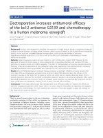
In the Aegean Sea cores, the SST values obtained
from Mg/Ca ratios agree closely with summer SST values
calculated using transfer functions (Figure 12). Mg/Ca
ratios were obtained from G. ruber, which is a warmwater indicator and has been used to estimate summer
seawater paleotemperatures. Both SST estimators support
the presence of cooler surface waters (at least during
summer) during accumulation of sapropels S5, S4, S3, and
S1 (Figures 11 and 12). The presence of small percentages
of N. pachyderma (s) during these intervals supports this
interpretation (Figures 4–8).

33



İŞLER et al. / Turkish J Earth Sci
Transfer function
MAR03-28
0

MIS

20

Age (ka)

40
60
80

1

Z2
S1

2

Y2
Y5

3

SST (°C) Transfer function

140


Z2
S1

A
B

Y5

C

S3

D

S3

E

5c

S4

S5

6

X1

F

G

5e

C

Nis

4
5a

8 12 16 20 24 28

A
B

Y2

SSTs

SSTs

Mg/Ca
SST (°C)

SST (°C)
8 12 16 20 24 28

Nis


5d
120

SST (°C)

MAR03-02

4 8 12 16 20 24 28 4 8 12 16 20 24 28

5b
100

Transfer function

Mg/Ca
SST (°C)

S4

1

F
G

SSTw

SSTw

H
I


D
E

1

2 345

Mg/Ca (mmol/mol)
2 345

Mg/Ca (mmol/mol)
30
28
26
24
22
20
18
16
14
12
10
8
6
4
2
0

y= 1.331 x - 6.147

r 2 = 0.95

SSTs
SSTw
y= 1.137 x - 8.578
r 2= 0.92

10

12

14

16

18

SST (°C) Mg/Ca

20

22

24

26

28

Figure 12. Comparison of the sea surface temperatures calculated using the planktonic foraminiferal transfer functions and Mg/Ca in

cores MAR03-28 and MAR03-02. Grey and yellow envelopes show the calculated values with error bars. Core locations are shown in
Figure 1.

Transfer function temperature variations during
transitions from interstadials to stadials of MIS 5 show
large amplitude fluctuations of 9–10 °C in cores MAR03-28
and MAR03-03, whereas in cores MAR03-02 and MAR0325 these variations are smaller at 3–5 °C. The fluctuations
are similar to those reported by van der Meer et al. (2007).
However, temperature fluctuations of 9–10 °C exceed
what would be expected for oxygen isotopic changes of
~1.2‰ during transitions (e.g., MIS 5d/5c), assuming that
the isotopic ratio changes by ~0.2‰ δ18O/°C (e.g., Emeis
et al., 2000). The percentage of N. pachyderma (d) tests

34

(subpolar species) in cores MAR03-28 and MAR03-03
is at least 20% higher than in other cores, and it is these
abundance peaks that account for the higher amplitude
temperature variations (~10 °C) in these cores. These large
shifts might be overestimates and the smaller fluctuations
based on Mg/Ca ratios (~4 °C; Figure 12) are thought to
be more accurate.
It is interesting that the paleotemperature estimates
based on both faunal and Mg/Ca data indicate cooling
during the sapropel deposition during MIS 5. This cooling
trend, particularly the one that is associated with the


İŞLER et al. / Turkish J Earth Sci

MIS 5e, is challenging because during this period the
summer insolation values were at their maximum (Berger,
1978; Berger et al., 2005, 2006). There are two possible
explanations for the observed SST and SSS trends: (i)
the faunal paleotemperature results are heavily biased by
increases in N. pachyderma (d) and/or by variations in sea
surface salinities, leading to low reliability in the trends,
or (ii) these trends are correct and the landlocked Aegean
Sea indeed experienced cooling during the deposition of
the MIS 5 sapropels. As a caveat, freshwater/nutrient input
from both the northern and eastern rivers draining into
the region, as well as freshwater influx from the south
associated with intensified African monsoons, might
have altered the salinity structure of the Aegean Sea, thus
potentially influencing the Mg/Ca ratio in foraminiferal
calcite (Ferguson et al., 2008). However, decreases in sea
surface temperatures of 2 °C for sapropel S5 and 6 °C for
S4 determined for the eastern Mediterranean Sea core
MD84-641 collected off the Nile River (Kallel et al., 2000)
are consistent with our results and suggest that the faunal
and Mg/Ca paleotemperatures reported here are correct.
4. Discussion
4.1. Significance of downcore distribution of G. bulloides
G. bulloides is one of the more dominant planktonic
foraminiferal species in the Mediterranean region,
including the Aegean and Adriatic seas. This species
tolerates a wide spectrum of temperatures and inhabits a
broad depth range, generally in the upper 100–200 m of

-1


MAR03-3

MAR03-25

the water column. It is an indicator of eutrophic waters and
upwelling (Rohling et al., 1993, 1997; Zaric et al., 2005).
During sapropel S1 deposition, higher abundances
of both G. bulloides and G. ruber (white) are observed
throughout the Aegean and the Adriatic seas and are
ascribed to either elevated nutrient concentrations in
surface waters due to enhanced river runoff or lower oxygen
content within the photic zone as a result of phyto and
zooplankton blooms (Rohling et al., 1993; Principato et al.,
2003; Geraga et al., 2005). The covariation of G. bulloides
and G. ruber (white) during sapropel S1 deposition is
supported by our work (Figures 4–8 and 13). Surprisingly,
however, increased abundances of both species correlate
with nonsapropel intervals at greater depths, particularly
in the hemipelagic muds between sapropels S3, S4, and
S5, which accumulated during MIS 5 (Figures 4–8). This
difference in the behaviour of G. bulloides and G. ruber
(white) between S1 and older sapropels S3, S4, and S5
indicates a significant difference in nutrient levels and
structure of the water column from MIS 5 to MIS 1.
Because G. bulloides and G. ruber are known to inhabit
eutrophic and oligotrophic waters, respectively, their
cooccurrence is potentially problematic and is discussed
further, below (under Ecozone IV).
4.2. Significance of downcore distribution of N.

pachyderma (d)
N. pachyderma (d) is either absent or has very low
percentages in sapropel S1, whereas the older sapropels

MAR03-28

MAR03-27

MAR03-2

-1

Warm
G. bulliodes
G. ruber (w)
O. universa
G. inflata
N. pachyderma (s)
T. quinqueloba
G. glutinata
G. scitula
N. dutertrei
N. pachyderma (d)

G. bulliodes
G. ruber (w)
Warm
O. universa
N. dutertrei
G. scitula

N. pachyderma (s)
N. pachyderma (d)
T. quinqueloba
G. inflata
G. glutinata

+1
Warm
G. bulliodes
O. universa
G. ruber (w)
G. inflata
G. glutinata
G. scitula
T. quinqueloba
N. pachyderma (d)
N. pachyderma (s)
N. dutertrei

+1
Warm
G. bulliodes
G. ruber (w)
O. universa
G. inflata
N. pachyderma (s)
T. quinqueloba
G. scitula
G. glutinata
N. dutertrei

N. pachyderma (d)

0

N. pachyderma (s)
T. quinqueloba
G. inflata
G. glutinata
N. dutertrei
N. pachyderma (d)
G. scitula
Warm
G. bulliodes
G. ruber (w)
O. universa

0

Figure 13. Dendrograms resulting from R-mode hierarchical cluster analysis (centroid linkage method, distance metric is 1-Pearson
correlation coefficient); warm = sum of tropical species.

35


İŞLER et al. / Turkish J Earth Sci
S3, S4, and S5 contain 50%–70% N. pachyderma (d). This
situation is also observed in other eastern Mediterranean
cores (e.g., Thunell et al., 1977; Rohling and Gieskes, 1989;
Rohling et al., 1993). N. pachyderma (d) is rare to absent
in oligotrophic waters, but its presence is well documented

in eutrophic waters closely associated with development
of a deep chlorophyll maximum. A deep chlorophyll
maximum develops when the pycnocline lies close to the
base of, or within, the euphotic zone where there is enough
light for primary production (Rohling and Gieskes, 1989;
Rohling et al., 1993). Rising of the pycnocline occurs when
the density contrast between the intermediate and surface
water decreases and, under such conditions, the nutricline
usually is found closely associated with the pycnocline.
In the modern Aegean Sea, the surface water layer
consists mainly of brackish Black Sea outflow, whereas
intermediate water is more saline Mediterranean
Intermediate Water. Hence, the pycnocline depth
(essentially a halocline) is regulated mainly by the
rate of freshwater/brackish water input, modulated by
evaporation and winter cooling. In this context, the
downcore frequency distribution of N. pachyderma (d)
can be interpreted as a record of the interactions between
surface and intermediate waters of the Aegean Sea, and
perhaps temporal changes in the end-member properties
of these water masses.
4.3. Significance of downcore distribution of stable
carbon isotopes (δ13C)
Inorganic carbon isotope signals reflect changes that
occurred within the surface water layer and, to a lesser
extent, the upper portions of the intermediate water
mass. This is where planktonic foraminifera dwell during
their life span. Theoretically, surface and deep waters
should display, respectively, heavier (most 13C enriched)
and lighter δ13CDIC values in the water column, because

12C is preferentially sequestered by marine algae during
photosynthesis within the euphotic layer and subsequently
transferred from the surface layers to deeper water by
postmortem settling of organic material (referred to as the
biological pump, Rohling et al., 2004). Foraminifera living
in such surface waters would form calcite tests enriched in
13C. However, in areas where enhanced river input occurs,
surface waters can exhibit depleted δ13C values due to the
light carbon content of the freshwater that can range from
–5‰ to –10‰ (inorganic carbon) to as light as –27‰
(suspended organic carbon; Fontugne and Calvert, 1992).
For example, the δ13C composition of the surface water
in the Black Sea is approximately –13‰ (Abrajano et al.,
2002). In semienclosed marine settings with significant
river inputs, the effect of biological pumping is masked
by light carbon dilution, and foraminifera are expected to
have depleted δ13C values.
In the studied cores, stable carbon isotopes in
planktonic foraminifera show maximum depletions

36

during and/or immediately below sapropels (Figure 10). If
biological pumping was the dominant control on surfacewater isotopic composition, then depleted planktonic
foraminiferal δ13C values might reasonably indicate low
primary productivity in the surface waters. However, the
Aegean Sea is surrounded by numerous freshwater/brackish
water sources, and so the light carbon isotopic values in
the foraminiferal tests cannot be used to assess changes in
primary productivity, and more likely record changes in

freshwater/brackish water supply. Uninterrupted presence
of benthic foraminifera in all samples, including sapropels,
strongly suggests that bottom waters were not anoxic,
but reached dysoxic levels. During the deposition of the
MIS 5 sapropels S3, S4, and S5, the notable depletion in
benthic foraminiferal δ13C values can be explained by
minor amounts of vertical mixing with depleted δ13CDIC
from the surface waters, leading to a degree of ventilation
(oxygenation) that prevented bottom-water anoxia.
4.4. Ecozones
Stratigraphic trends in the distribution of the most
common taxa (N. pachyderma (d), G. bulloides, G. ruber,
G. inflata) are very similar in all five cores studied from
the Aegean Sea, suggesting that major changes in surfacewater characteristics took place more or less synchronously
throughout the Aegean Sea since ~130 ka.
Ecozone IV (>60 ka)
Ecozone IV spans a time interval during which
successive moderate amplitude fluctuations are observed
in SST, SSS, and δ13C values, and in the frequency
distributions of the most common taxa (i.e. N. pachyderma
(d), G. ruber, and G. bulloides). Sapropels S3, S4, and S5
accumulated under these conditions (Figures 4–11). A
close covariation of G. ruber and G. bulloides is consistently
observed during deposition of nonsapropel sediments
within Ecozone IV (Figure 14a). G. ruber is a warm
oligotrophic mixed-layer dweller, whereas G. bulloides is
highly dependent on enhanced food levels with no depth
preference. The covariation is consistent with stratification
of the euphotic zone, with a warmer and nutrient-poor
upper layer and a cooler lower layer with high nutrient

content. Such conditions could provide favorable habitats
for both species to thrive at slightly different depths in
the water column. The dominance of N. pachyderma
(d) during times of sapropel formation indicates the
establishment of a sustained and distinct deep chlorophyll
maximum layer within the euphotic zone (Figures 14b and
14c). Such conditions require stratification of the water
column and shoaling of the pycnocline into the euphotic
ecozone. The formation of a deep chlorophyll maximum
layer is promoted by increased river runoff, which is
consistent with decreased sea surface temperatures and
the observed depletions in δ13C values. Another important
observation is the close association of N. dutertrei with


İŞLER et al. / Turkish J Earth Sci

a

river input
12
MIS5 sapropels S3, S4, S5 rich in C

d

24°C - 26°C

_ _

_ _


sapropel S1

23°C - 24°C

_ _

Photic zone

pre-sapropel
post-sapropel

b
DCM
layer

nutricline
_O_2
20°C - 23°C

_ _

_ _

_ _

{

onset of sapropel
S3, S4, S5 deposition


_ __ _

e

maximum TOC
accumulation
(sapropels S3, S4, S5)

_ _

Ecozone III
12°C - 16°C

non sapropel intervals

_ _

f

O2

8°C - 12°C

Glacial intervals

Photic zone

Intermediate


dysoxic

N. pachyderma (d)
G. ruber
G. bulloides
G. glutinata

_ _

24°C - 26°C

Bottom

_ _

_ _

?
dysoxic

Photic zone

14°C - 17°C

{

_ _

Ecozone IV


?

Intermediate

dysoxic

c
DCM
layer

Bottom

_ _

_ _

?

Intermediate

river input
rich in 12 C

_ _
Bottom

G. inflata
N. dutertrei
O 2 oxic
sapropel


_ _

O2

export production

SST summer

stagnation
pycnocline/nutricline

sluggish
well mixed

_ _ depleted δ13 C signature

Figure 14. Schematic demonstration of water column hydrographic conditions during the formation of sapropels S3, S4, and S5 (part
a = presapropel and postsapropel, part b = sapropel onset, part c = height of sapropel development); sapropel S1 (part d); nonsapropel
layers (part e), and glacial times (part f). Green tone marks deep chlorophyll maximum.

sapropels S3, S4, and S5 and the peak abundances of N.
pachyderma (d). The subsurface-dwelling foraminifera N.
dutertrei is exclusively herbivorous and so its population
increases after phytoplankton blooms (Thunell and
Reynolds, 1984; Hemleben et al., 1989). The appearance
of N. dutertrei during times of maximum abundances of
N. pachyderma (d) might record the shallowest position
of the deep chlorophyll maximum layer, well into the
euphotic zone, when large phytoplankton populations

would be expected (Figure 14c). In addition, the highest
organic carbon concentrations also coincide with the
presence of N. dutertrei, suggesting a positive correlation

between shoaling of the deep chlorophyll maximum and
enhanced organic carbon deposition. The presence of
G. inflata in sapropel S4 in all cores studied is a notable
difference in the MIS5 sapropels (Figures 4 and 6–8). The
persistent and relatively high abundances of G. inflata in
the cores from the Aegean Sea strongly suggest enhanced
vertical mixing, at least during the winters (i.e. Pujol and
Vergnaud-Grazzini, 1995).
The development of a deep chlorophyll maximum
layer during the deposition of sapropels S3, S4, and S5
has been suggested for the southernmost Aegean Sea
by other researchers (Rohling and Gieskes, 1989). Core

37


İŞLER et al. / Turkish J Earth Sci
T87/2/27 is a 3-m-long gravity core that was collected
immediately southwest of the Island of Antikythera
(Figure 1; Rohling and Gieskes, 1989). Four sapropel/
sapropelic mud layers were identified in this core and were
tentatively correlated with the oxygen isotopic record of
RC-9 181, a core recovered from the Mediterranean Ridge
south of Crete (33°25ʹN & 25°00ʹE – 2286 m water depth;
Vergnaud-Grazzini et al., 1977). Rohling and Gieskes
(1989) correlated these sapropels with S1, S3, S4, and S5

and suggested that the absence of neogloboquadrinids in
S1 and their abundance in S3, S4, and S5 reflect differences
in food availability related to the extent of development
of a deep chlorophyll maximum layer and the intensity of
primary production associated with this layer. They argued
that the depth of the deep chlorophyll maximum layer is
determined by the vertical structure of the water column,
and suggested that the pycnocline was positioned well
above the base of the euphotic zone during deposition of
sapropels S3, S4, and S5. Core LC21 is a 13.5-m-long piston
core collected from the eastern Cretan Trough, west of the
islands of Kasos and Karpathos (Figure 1; Rohling et al.,
2004; Marino et al., 2009; Osbourne et al., 2010). This core
has been the focus of extensive paleoceanographic research
and has become the best understood sapropel record in the
eastern Mediterranean Sea (Rohling et al., 2004; Marino et
al., 2009; Osbourne et al., 2010). Sapropels S1 and S3–S5
were identified in LC21, although previous studies have
generally focused on sapropels S1 and S5, with no major
work on sapropels S3 and S4. The chronostratigraphy of
the core was established through radiocarbon dating in
the upper part of the core and by correlation to the Soreq
Cave speleothem data (Bar-Matthews et al., 2003; 2009)
for the age of S5. Previous studies showed that sapropel
S5 accumulated under conditions of enhanced freshwater
dilution of surface waters, elevated productivity, shoaling
of the pycnocline between intermediate and surface waters,
and stagnation of the subsurface circulation (Rohling et
al., 2004). Freshwater contributions to the Aegean Sea
during the deposition of sapropel S5 were traced using

Nd isotopes in planktonic foraminifera (Osbourne et
al., 2010), possible because radiogenic sources are most
widespread to the south, in Africa, whereas nonradiogenic
sources are found to the north. These data showed that
the most likely source for freshwater was rivers flowing
northward from the central Saharan watershed. Osbourne
et al. (2010) concluded that there was no large influx of
water from the north during the deposition of sapropel S5.
During the formation of MIS 5 sapropels S3, S4, and
S5, δ18O and sea surface temperature/salinity values show
contradictory relationships: depletions in oxygen isotope
values coincide with decreased SST and SSS values.
Although not commonly observed, drops in sea surface
temperatures of 2 °C (S5) and 6 °C (S4) have also been

38

observed from the eastern Mediterranean Sea in core
MD84-641 collected off the Nile River where increasing
surface temperatures are associated with δ18O enrichments
in the planktonic foraminifera G. ruber (Kallel et al., 2000).
The association of lower SST/SSS values with more negative
δ18O values in the cores can be attributed to the presence
of less saline cool waters and/or increased precipitation.
In this study, benthic foraminiferal assemblages are not
described in detail; however, benthic foraminifera were
examined in samples from sapropels S3, S4, and S5. These
samples contained a low-abundance and low-diversity
benthic foraminiferal fauna dominated by Globobulimina
affinis, G. pseudospinescens, Chilostomella mediterranensis,

Bolovina alata, B. attica, Bulimina clara, and Uvigerina
peregrina curticosta. This benthic foraminiferal faunal
assemblage indicates nutrient-rich, oxygen-poor bottom
waters during the deposition of MIS 5 sapropels S3, S4, and
S5. G. affinis, G. pseudospinescens, and C. mediterranensis
co-occurring with Bolivina species are also reported in
several sapropels from the eastern Mediterranean Sea
(Cita and Podenzani, 1980; Herman, 1981; Mullineaux
and Lohmann, 1981; Stefanelli et al., 2005; Abu-Zied et al.,
2008; Melki et al., 2010) and are known to be abundant in
oxygen-poor (dysoxic) bottom water conditions (Ross and
Kennett, 1984; McCorkle et al., 1990; Stefanelli et al., 2005;
Abu-Zied et al., 2008; Melki et al., 2010).
The depleted planktonic and benthic δ13C values
are interpreted to be a consequence of river runoff
bringing 12C-enriched nutrients, and a distinct deep
chlorophyll maximum layer situated well within the
euphotic layer providing additional nutrients that resulted
in augmented 12C-enriched ‘export’ to the sea floor
(Figure 14c). Furthermore, close covariation between
benthic and planktonic δ13C signals suggests that deep
waters inherited their carbon from surface waters via
the export of organic detritus from the upper part of the
water column and limited vertical mixing. Coincident
depletions/enrichments both in carbon and oxygen
isotope values support the hypothesis that fluvial 12C- and
16O-enriched waters controlled the isotopic composition
in the semienclosed Aegean Sea.
Pollen records, both terrestrial (i.e. Ionnina - western
Greece, Tenaghi Philippon - northeastern Greece;

Mommersteeg et al., 1995; Tzedakis et al., 1997, 2006) and
marine (MD84-627 and MD84-642 - northeast off the Nile
River), show that climatic conditions during interstadials
were humid and warm, characterized by high abundances
(to 97%) of arboreal pollen (e.g., Quercus, Pinus, Pistacia
Figure 15), whereas stadials were cooler and more arid
(e.g., increase in Artemisia; Tzedakis et al., 1997; Cheddadi
and Rossignol-Strick, 1995; Mommersteeg et al., 1995).
Maximum depletions in the foraminiferal δ13C and δ18O
signals in the Aegean Sea cores are in good agreement


İŞLER et al. / Turkish J Earth Sci

A
0
20

Age (ka)

40
60
80

MIS
1

S1

3


140

-1

0

5

1

4

3

2

1

0

C
-1 5.4

4

5.8

6.2


0

D
25

E

AP%
50

75 100 -2

F

Soreq δ18Ospeleo (‰) Quercus Artemisia
-4

-6

-8

0

20

0

20

warm/humid


S2
S3
stacked
benthic

stacked
benthic

5c

5e

Precession (º)

stacked
planktonic

5a

5d
120

-2

δ18 O (‰ PDB)
G. ruber

2


5b S4
100

B

δ13 C (‰ PDB)
G. ruber

S5

stacked
planktonic

6

0

1

2

U. mediterranea
δ13 C (‰ PDB)

3

5

4


3

2

1

0

U. mediterranea
δ18 O (‰ PDB)

-1

cold/dry
140
150
160

Figure 15. Comparison of stacked δ13C and δ18O curves from this study with pollen records from NE Greece and the eastern
Mediterranean. (A) stacked δ13C curves in planktonic and benthic foraminifera; (B) stacked δ18O curves in planktonic and benthic
foraminifera; (C) precession curve; (D) arboreal pollen (AP) percentage curve from Tenaghi Philippon sequence, NE Greece (modified
from Tzedakis et al., 2003); (E) Soreq Cave δ18Ospeleo record (modified from Grant et al., 2012); (F) downcore variations of Quercus
and Artemisia species (wet/warm-forest and arid/cool climate indicators, respectively) in MD84-627 (off the Nile River; modified from
Cheddadi and Rossignol-Strick, 1995).

with increased arboreal pollen percentages particularly
during interstadial stage 5a. However, rather ‘short lived’
isotopic depletions during the deposition of sapropels S5
and S4 do not reflect the extended periods of high arboreal
pollen encompassing the entire interstadial stages 5e and

5c. Instead, the depletions coincide well with times of
maximum insolation (with ~3 kyr lag) suggesting that the
intensity of the monsoon system played an important role
in the climatic conditions over the Aegean Sea (Figure 15).
There is also a remarkable correlation between the ~150
kyr δ18O and δ13C record determined from speleothems
of the Peqiin Cave in Israel and the stable isotopic records
from the Aegean Sea cores (Figure 15; Bar-Matthews et
al., 2003; Grant et al., 2012). This correlation provides a
strong linkage between the regional terrestrial climatic
signal, reflecting the variations in land temperature and
rainfall, and the oceanic climate reflected in SSTs, SSTw,
and SSSw records. The correspondence of low δ18O
speleothem values with low G. ruber δ18O values in the
Aegean Sea cores during interglacial sapropel events S3,
S4, and S5 indicates that these periods were characterized
by enhanced rainfall in the eastern Mediterranean region,
over both land and sea (Figure 15; Bar-Matthews et al.,
2003; Grant et al., 2012).
In the eastern Mediterranean Sea, the MIS 5 sapropels
were deposited during substages 5a (sapropel S3), 5c
(sapropel S4), and 5e (sapropel S5) and are in some
instances associated with δ18O depletions and increased
sea surface temperatures (e.g., Mulitza et al., 2003) and in

other instances with decreased sea surface temperatures
(e.g., Kallel et al., 2000). Similarly, depleted oxygen isotope
values are observed in MIS 5 sapropels from the Aegean
Sea (Figures 9, 11, and 12). However, the planktonic
foraminiferal δ18O values are more enriched than in

their counterparts from the eastern Mediterranean Sea,
corresponding to ~5 °C lower sea surface temperatures
(Figures 11 and 12), and are more similar to core MD84641 off the Nile River (Kallel et al., 2000). This enrichment
is probably caused by temperature differences rather than
by higher salinity considering the confined geographic
position of the Aegean Sea and the high fresh/brackish
water input by the surrounding rivers and Black Sea
outflow. If true, these enriched δ18O signals support the
presence of cooler surface waters during the formation of
MIS 5 sapropels in the Aegean Sea with respect to those in
the eastern Mediterranean Sea.
Ecozone III (60–40 ka)
The reappearance of G. inflata and decreased
percentages of N. pachyderma (d) in ecozone III indicate
a weaker stratification of the surface waters than was the
case for subecozone IVa (Figure 14d). In the southern
cores MAR03-25 and MAR03-02, higher abundances
of G. inflata reaching 36% and low abundances of N.
pachyderma (d) together suggest the presence of a stronger
vertical mixing of the surface waters than at other core
localities. These hydrographic conditions show similarities
to those that existed during nonsapropel times in Ecozone
IV (see above); however, the SST values for Ecozone III

39


İŞLER et al. / Turkish J Earth Sci
are significantly lower by as much as 4 °C, consistent with
relatively enriched δ18O signatures and lower G. ruber

abundances.
Higher percentages of N. pachyderma (d) and T.
quinqueloba at the upper and lower boundaries of Ecozone
III suggest cooler and less saline surface waters, confirmed
by SST and SSS plots (Figure 11). G. glutinata appears for
the first time within the upper portions of Ecozone III,
signaling the initial stages of glacial conditions associated
with the transition into MIS 2. Furthermore, the SST plots
show that the temperature drop of 2–4 °C toward the top
of the ecozone is more pronounced than the earlier drop at
the lower boundary (Figure 11).
Ecozone II (40–12.5 ka)
During the development of Ecozone II, the upward
increase in the abundance of N. pachyderma (d) together
with the presence of N. pachyderma (s) and T. quinqueloba
indicate progressive cooling into a cold interval
corresponding to the glacial MIS 2 (Figure 14e). This
climatic change is also demonstrated by enrichment in
δ18O values and decreased surface water temperatures. The
planktonic foraminiferal SST and Mg/Ca SST calculations
show that water temperatures ranged between 11 °C and
15 °C, about 6 °C cooler than today (Figure 12). Ecozone
II demonstrates similar frequency distributions (e.g.,
dominance of N. pachyderma (d), decreased G. ruber and
G. bulloides percentages) to those observed in subecozones
IV a, c, and e, suggesting that similar water masses existed
during glacial periods and during times of formation of
sapropels S3, S4, and S5 (Figures 11, 14e versus 14b).
An important difference in Ecozone II is that
sedimentation took place under oxygenated bottom

water conditions unfavorable for increased organic
carbon preservation (Figure 14e). The dominance of N.
pachyderma (d) during MIS 2 places constraints on the
conditions prevailing during the deposition of MIS 5
sapropels. During MIS 2 as well as the sapropel intervals
of MIS 5 there was a permanent pycnocline within
the euphotic zone, and the density contrast between
intermediate and surface waters was of similar magnitude.
The proposed shallow position of the permanent
pycnocline during MIS 2 can be explained by glacioeustatic
sealevel lowering, as has been hypothesized for the eastern
Mediterranean Sea (Rohling and Gieskes, 1989; Rohling,
1991). There, a shallow permanent pycnocline and related
frequency increases in neogloboquadrinids during glacial
periods are attributed to glacioeustatic sealevel lowering
that resulted in a reduction in inflow across the Strait of
Sicily (Rohling, 1991). Similar conditions could easily be
envisaged for the semienclosed Aegean Sea where reduced
inflow from the eastern Mediterranean Sea and the Black
Sea could cause comparable conditions with less buoyancy
contrast between the surface and the intermediate waters,

40

resulting in a shallower pycnocline. Episodic appearances
of G. inflata, an indicator of a cool and homogeneous
winter mixed layer, during the formation of MIS 5
sapropels and its complete absence throughout Ecozone II
are suggestive of a sustained/stronger stratification of the
water column particularly during glacial times (e.g., MIS

2). However, the fact that bottom water oxygen deficiency
did not develop throughout the entire glacial time span
implies that surface water temperatures were sufficiently
low to promote downwelling, permitting bottom water
replenishment, and accordingly precluding sapropel
formation.
Ecozone I (12.5 ka–present)
The dominance of G. ruber in Ecozone I together
with relatively high abundances of warm water species
indicates the establishment of fully interglacial conditions
(Figure 14f). The SST calculations support the presence
of warm waters that mainly ranged between 17 °C and 24
°C (Figures 11 and 12). Rohling and Gieskes (1989) also
suggested that during the deposition of sapropel S1 the
pycnocline vanished due to termination of Mediterranean
Intermediate Water formation and that there was no deep
chlorophyll maximum. Significant depletions in δ13C
values, particularly during sapropel S1 accumulation,
suggest excessive amounts of freshwater and/or brackish
water input to the Aegean Sea, most likely from the Black
Sea and rivers draining into the Black Sea and possibly
in lesser amounts from the Nile River (Figure 10). Other
workers also have suggested that fresh/brackish water
outflow from the Black Sea during the MIS 2/1 transition
is mainly responsible for the development of sapropel S1
(Aksu et al., 1995; Hiscott et al., 2007a, 2007b).
The above interpretation requires that the Black Sea
was connected to the Aegean Sea through the Marmara
Sea at, or immediately before, the onset of deposition of
the most recent sapropel S1. The late MIS 2 and Holocene

reconnection of the Black Sea to the world ocean is hotly
debated in the literature. Hiscott et al. (2007a, 2007b)
have provided arguments supporting persistent Black
Sea outflow to the world ocean starting at ~11.7 cal ka,
including the period of M1 and S1 sapropel deposition in
the Marmara and Aegean seas, ~11.9–6.75 cal ka (Çağatay
et al., 2000) and ~9.9–6.6 cal ka respectively. Thom (2010)
modeled the hydrological budget of the Black Sea through
the late Quaternary and concluded that the Black Sea must
have been exporting water to the world ocean during S1
time. Other workers have disagreed based on isotopically
based estimates of SST and SSS using alkenone biomarkers
and oxygen isotopic variations (Sperling et al., 2003; Vidal
et al., 2010), noting higher SSS values during M1/S1 time
that are apparently inconsistent with Black Sea outflow.
Vidal et al. (2010) suggested that the Marmara Sea only
became reconnected to the Black Sea between 9 and 8 cal


İŞLER et al. / Turkish J Earth Sci
ka, ~1000 years after the onset of sapropel deposition in
the Aegean Sea. Çağatay et al. (2009) have provided an
explanation for sapropel M1 in the Marmara Sea that has
no genetic link with conditions that led to the deposition
of essentially coeval S1 in the Mediterranean Sea and no
link with Black Sea outflow. They proposed that intrusion
of saline Mediterranean water, starting at ~13.4 cal ka
(calibrated from ~12 14C ka) forced the ambient fresher
waters to the surface and eventually out through the
Dardanelles Strait, creating water-column stratification

and bottom-water dysoxia in the Marmara Sea that, with a
significant time lag, promoted sapropel formation.
The assessments by Sperling et al. (2003) and Vidal
et al. (2010) of a higher, rather than lower, SSS in the
Marmara Sea during S1 deposition in the Aegean Sea
might not actually rule out Black Sea outflow at that time.
This is because the isotopic data underpinning the SSS
estimates come from the remains of marine algae and
foraminifera that do not tolerate the low salinity of surface
waters in the Marmara Sea, even today when those surface
waters have a salinity of ~20 psu down to a depth of ~25
m (Aksu et al., 2002). Vidal et al. (2010) proposed that
these organisms lived in the region of the contemporary
pycnocline, but if the SSS estimates recently published by
Mertens et al. (2012) and Bradley et al. (2012) are correct,
then any early Holocene Black Sea outflow would have had
a significantly lower salinity of ~7–14 psu, effectively toxic
to the marine organisms used by Sperling et al. (2003)
and Vidal et al. (2010) for their SSS estimates. Hence,
their alkenone and oxygen-isotopic data must record the
water temperature and salinity within the top of the saline
deeper water mass of the Marmara Sea, above which a
low-salinity sheet of Black Sea outflow might have been
flowing, undetected by their methods, toward the Aegean
Sea. Until there is stronger, unambiguous evidence that
Black Sea outflow could not have been possible during S1
time, the interpretation presented in this paper to explain
the creation of a low-salinity lid preventing bottom-water
ventilation in the Aegean Sea remains viable. Furthermore,
the genesis of largely contemporaneous sapropels M1

and S1 can be explained in a consistent manner if Black
Sea outflow was a trigger, rather than needing fully
independent mechanisms for similar and synchronous
organic-rich deposits in such close geographic proximity.
The notable drop in δ13C values during the deposition
of sapropel S1 coincides with only minor cooling of
surface water temperatures (Figure 11). The lack of
greater cooling at this time can be ascribed to the warmer
temperatures of the Black Sea outflow into the Aegean
Sea, as surface waters likely warmed while flowing
across the Marmara Sea on their way to the Aegean Sea
(Poulos et al., 1997; Zervakis and Georgopoulos, 2002).
The abrupt disappearance of N. pachyderma (d) during

deposition of S1 suggests unfavorable conditions for the
development of a deep chlorophyll maximum layer. This
might have been caused by deepening of the pycnocline
far below the euphotic ecozone (Figure 14f) or even by
complete disruption of the pycnocline. This situation
would require a near-complete shutdown of intermediate
water formation, causing a diminished oxygen supply at
intermediate depths, thus resulting in strongly stagnant
bottom water conditions (e.g., Rohling and Gieskes, 1989).
Increased abundances of G. bulloides during deposition of
S1 have also been recognized in the Adriatic Sea (Jorissen
et al., 1993; Rohling et al., 1993) and by other workers in
the Aegean Sea (e.g., Geraga et al., 2010) and have been
attributed by those authors to increased river discharges
creating high nutrient levels.
Stratification occurs in the water column when there

is a high density contrast between the surface mixed layer
and the intermediate and/or bottom waters. Stagnation
can take place locally in bottom waters where there is
strong vertical stratification. A stratified water column
would diminish or even halt the vertical advection of
oxygenated surface waters resulting in sluggish/stagnant
bottom waters. In shallow basins with a thin surface layer,
stratification can be broken during intense storms, which
would cause the thermocline/nutricline to rise well within
the surface mixed layer. As a result, nutrient-rich waters
would increase the rate of photosynthesis, enhancing
primary production. Stagnation can also occur in regions
where there is a marked reduction (or cessation) in the rate
of bottom water formation.
Quantitative variations in the planktonic faunal
assemblages identified in five cores collected from the
northern to southern Aegean Sea support the following
conclusions. Sapropels S3, S4, and S5 were deposited
under similar hydrographic conditions with a distinct
deep chlorophyll maximum layer, a stratified water
column, and increased primary productivity. Sapropel
S1 was deposited in the absence of a deep chlorophyll
maximum layer, so that the water column lacked a deep
phytoplankton assemblage. Under such conditions,
oxygen advection via intermediate water flow must have
been significantly reduced, which implies significant
stagnation. Leading up to the deposition of sapropels S3,
S4, and S5, modifications in the hydrographic conditions
were initiated ~5–7 kyr before the onset of sapropel
deposition. The sapropels predominantly coincided with

maximum depletions in δ13C and lowest SST values. The
dominant factor for the formation of MIS 5 sapropels was
an increase in primary productivity; however, the presence
of sluggish intermediate water with weakened bottom
water replenishment cannot be discounted. The formation
of sapropel S1 is attributed to intense fresh/brackish water
input, which resulted in strong stratification and the near
stagnation of the bottom water.

41


İŞLER et al. / Turkish J Earth Sci
Cluster analysis shows consistent coupling of G.
bulloides with G. ruber during times of nonsapropel
deposition, which is interpreted to suggest a stratified
euphotic zone composed of a warm/nutrient-poor and a
cooler/nutrient-rich upper and lower layer, respectively.
This covariation further points to increased river runoff
to explain the fertility and stratification of the surface
waters. In sapropel layers S3, S4, and S5, appearances of N.
dutertrei are interpreted to represent maximum shoaling of
the pycnocline and highest levels of primary productivity.

Acknowledgements
We thank Dr Doğan Yaşar for his continued support and the
officers and crew of the RV Koca Piri Reis of the Institute of
Marine Sciences and Technology, Dokuz Eylül University,
for their assistance in data acquisition. We acknowledge
research and ship-time funds from the Natural Sciences

and Engineering Research Council of Canada (NSERC) to
Aksu and Hiscott, travel funds from the Dean of Science,
Memorial University of Newfoundland, and a special grant
from the Vice President (Research), Memorial University
of Newfoundland. We thank Alison Pye for her assistance
in the stable isotopic and elemental analyses.

References
Abrajano T, Aksu AE, Hiscott RN, Mudie PJ (2002). Aspect of carbon
isotope biogeochemistry of Late Quaternary sediments from
the Marmara Sea and Black Sea. Mar Geol 190: 151–164.
Abu-Zied RH, Rohling EJ, Jorissen FJ, Fontanier C, Casford JSL,
Cooke S (2008). Benthic foraminiferal response to changes
in bottom-water oxygenation and organic carbon flux in the
eastern Mediterranean during LGM to Recent times. Mar
Micropaleontol 67: 46–68.

Berger A (1978). Long-term variations of daily insolation and
Quaternary climate changes. J Atmos Sci 35: 2362–2367.
Berger A, Mélice JL, Loutre MF (2005). On the origin of the 100kyr cycles in the astronomical forcing. Paleoceanography, 20:
PA4019, doi:10.1029/2005PA001173.
Berger A, Loutre MF, Mélice JL (2006). Equatorial insolation: from
precession harmonics to eccentricity frequencies. Clim Past 2:
131–136.

Aksu AE, Yaşar D, Mudie PJ (1995a). Paleoclimatic and
paleoceanographic conditions leading to development of
sapropel layer S1 in the Aegean Sea basins. Palaeogeogr
Palaeoecol 116: 71–101.


Bradley LR, Marret F, Mudie PJ, Aksu AE, Hiscott RN (2012).
Constraining Holocene sea-surface conditions in the
southwestern Black Sea using dinoflagellate cysts. J Quaternary
Sci 27: 835–843.

Aksu AE, Yaşar D, Mudie PJ, Gillespie H (1995b). Late glacial Holocene paleoclimatic and paleoceanographic evolution
of the Aegean Sea: micropaleontological and stable isotopic
evidence. Mar Micropaleontol 25: 1–28.

Çağatay MN, Görür N, Algan A, Eastoe CJ, Tchapalyga A,
Ongan D, Kuhn T, Kuscu I (2000). Late Glacial – Holocene
palaeoceanography of the Sea of Marmara timing of
connections with the Mediterranean and the Black Sea. Mar
Geol 167: 191–206.

Aksu AE, Hiscott RN, Mudie PJ, Rochon A, Kaminski M, Abrajano
T, Yaşar D (2002). Persistent Holocene outflow from the Black
Sea to the eastern Mediterranean contradicts Noah’s Flood
hypothesis. GSA Today 12: 4–10.
Aksu AE, Jenner G, Hiscott RN, İşler EB (2008). Occurrence,
stratigraphy and geochemistry of Late Quaternary tephra
layers in the Aegean Sea and the Marmara Sea. Mar Geol 252:
174–192.
Anand P, Elderfield H, Conte MH (2003). Calibration of Mg/
Ca thermometry in planktonic foraminifera from a
sediment trap time series, Paleoceanography 18: 1050,
doi:10.1029/2002PA000846.
Bar-Matthews M, Ayalon A, Gilmour M, Matthews A, Hawkesworth
CJ (2003). Sea–land oxygen isotopic relationships from
planktonic foraminifera and speleothems in the Eastern

Mediterranean region and their implication for paleo-rainfall
during interglacial intervals. Geochim Cosmochim Ac 67:
3181–3199.
Bé AWH, Spero HJ, Anderson OR (1982). Effect of symbiont
elimination and reinfection on the life processes of the
planktonic foraminifera Globigerinoides sacculifer: Mar Biol 70:
73–86.

42

Çağatay MN, Eriş K, Ryan WBF, Sancar U, Polonia A, Akçer S,
Biltekin D, Gasperini L, Görür N, Lericolais G et al. (2009).
Late Pleistocene-Holocene evolution of the northern shelf of
the Sea of Marmara. Mar Geol 265: 87–100.
Casford JSL, Rohling EJ, Abu Zied RH, Cooke S, Fontanier C, Leng
M, Lykousis V (2002). Circulation changes and nutrient
concentrations in the late Quaternary Aegean Sea: a nonsteady state concept for sapropel formation. Paleoceanography
17: 1024, DOI:10.1029/2000PA000601.
Cheddadi R, Rossignol-Strick M (1995). Improved preservation of
organic matter and pollen in Eastern Mediterranean sapropels.
Paleoceanography 10: 301–309.
Cita MB, Podenzani M (1980). Destructive effects of oxygen
starvation and ash falls on benthic life: a pilot study. Quaternary
Res 13: 230–241.
Dekens PS, Lea DW, Pak DK, Spero HJ (2002). Core top
calibration of Mg/Ca in tropical foraminifera: refining
paleotemperature estimation. Geochem Geophys Geosys 3:
1022, doi:10.1029/2001GC000200.
Edgar KM, Bohaty SM, Gibbs SJ, Sexton PF, Norris RD, Wilson PA
(2013). Symbiont ‘bleaching’ in planktic foraminifera during

the Middle Eocene Climatic Optimum. Geology 41: 15–18.


İŞLER et al. / Turkish J Earth Sci
Emeis KC, Schulz H, Struck U, Rossignol-Strick M, Erlenkeuser
H, Howell MW, Kroon D, Mackensen A, Ishizukam S,
Oba T et al. (2003). Eastern Mediterranean surface water
temperatures and δ18O composition during deposition of
sapropels in the late Quaternary. Paleoceanography 18: 1005.
doi:10.1029/2000PA00061.

Hiscott RN, Aksu AE, Mudie PJ, Marret F, Abrajano T, Kaminski
MA, Evans J, Çakıroğlu A, Yaşar D (2007b). A gradual
drowning of the southwestern Black Sea shelf: evidence for a
progressive rather than abrupt Holocene reconnection with the
eastern Mediterranean Sea through the Marmara Sea Gateway.
Quatern Int 167: 19–34.

Emeis KC, Sakamoto T, Wehausen R, Brumsack HJ (2000). The
sapropel record of the eastern Mediterranean Sea—results of
Ocean Drilling Program Leg 160. Palaeogeogr Palaeoecol 158:
371–395.

Imbrie J, Kipp NG (1971). A new micropaleontological method for
quantitative paleoclimatology application to a late Pleistocene
Caribbean core. In: Turekian KK editor. The Late Cenozoic
Glacial Ages. New Haven, CT, USA: Yale University Press, pp.
71–182.

Facorellis Y, Maniatis Y, Kromer B (1998). Apparent 14C ages of

marine mollusk shells from a Greek island: calculation of the
marine reservoir effect in the Aegean Sea. Radiocarbon 40:
963–973.
Ferguson JE, Henderson GM, Kucera M, Rickaby REM (2008).
Systematic change of foraminiferal Mg/Ca ratios across a
strong salinity gradient. Earth Planet Sc Lett 265: 153–166.
Fontugne MR, Calvert SE (1992). Late Pleistocene variability of the
carbon isotopic composition of organic matter in the eastern
Mediterranean: monitor of changes in carbon sources and
atmospheric CO2 concentrations. Paleoceanography 7: 1–20.
Geraga M, Tsaila Monopolis St, Ioakim Ch, Papatheodorou G,
Ferentinos G (2005). Short term climate changes in the
southern Aegean Sea over the last 48,000 years. Palaeogeogr
Palaeoecol 220: 311–332.
Geraga M, Ioakim Chr, Lykousis V, Tsalia-Monopolis St,
Mylona G (2010). The high-resolution palaeoclimatic and
palaeoceanographic history of the last 24,000 years in the
central Aegean Sea, Greece. Palaeogeogr Palaeoecol 287: 101–
115.
Grant KM, Rohling EJ, Bar-Matthews M, Ayalon A, Medina-Elizalde
M, Bronk Ramsey C, Satow C, Roberts AP (2012). Rapid
coupling between ice volume and polar temperature over the
past 150,000 years. Nature 491: 744–747.
Grimm EC (1987). CONISS: a FORTRAN 77 program for
stratigraphically constrained cluster analysis by the method of
incremental sum of squares. Comput Geosc 13: 13–35.
Hemleben C, Spindler M, Anderson OR (1989). Modern Planktonic
Foraminifera. Heidelberg, Germany: Springer Verlag.
Herman Y (1981). Paleoclimatic and paleohydrologic record of
Mediterranean deep-sea cores based on pteropods, planktonic

and benthic foraminifera. Rev Esp Micropaleontol 8: 171–200.
Hiscott RN, Aksu AE, Mudie PJ, Kaminski MA, Abrajano T, Yaşar
D, Rochon A (2007a). The Marmara Sea Gateway since ~16
ka: non-catastrophic causes of paleoceanographic events in
the Black Sea at 8.4 ka and 7.15 ka. In: YankoHombach V,
Gilbert AS, Panin N, Dolukhanov P editors. The Black Sea
Flood Question: Changes in Coastline, Climate, and Human
Settlement. NATO Science Series IV - Earth and Environmental
Sciences. Dordrecht, the Netherlands: Springer, pp. 89–117.

Jorissen FJ, Asioli A, Borsetti AM, Capotondi L, de Visscher JP,
Hilgen FJ, Rohling EJ, van der Borg K, Vergnaud Grazzini C,
Zachariasse WJ (1993). Late Quaternary central Mediterranean
biochronology. Mar Micropaleontol 21: 169–189.
Kallel N, Duplessy JC, Labeyrie L, Fontugne M, Paterne M, Montacer
M (2000). Mediterranean pluvial periods and sapropel
formation over the last 200 000 years. Paleogeogr Paleoecol
157: 45–58.
Kidd RB, Cita MB, Ryan WBF (1978). Stratigraphy of eastern
Mediterranean sapropel sequences recovered during DSDP
LEG 42A and their paleoenvironmental significance. In: Hsu
KJ, Mondrader L editors. Initial Reports of the Deep Sea
Drilling Project. US Government Printing Office, Washington,
DC, USA, pp. 421–443.
Lea DW, Pak DK, Spero HJ (2000). Climate impact of Late Quaternary
equatorial Pacific sea temperature variations. Science 289:
1719–1724.
Lea DW, Pak DK, Peterson LC, Hughen KA (2003). Synchroneity of
tropical and highlatitude Atlantic temperatures over the Last
Glacial Termination. Science 301: 1361–1364.

Lisiecki LE, Raymo ME (2005). A Pliocene-Pleistocene stack of 57
globally distributed benthic δ18O records. Paleoceanography
20: 1–17.
Margari V, Pyle D, Bryant C, Gibbard PL (2007). Mediterranean
tephra stratigraphy revisited: results from a long terrestrial
sequence on Lesvos Island, Greece. J Volcanol Geoth Res 163:
34–54.
Marino G, Rohling EJ, Sangiori F, Hayes A, Casford JL, Lotter AF,
Kucera M, Brinkhuis H (2009). Early and middle Holocene
in the Aegean Sea: interplay between high and low latitude
climate variability. Quaternary Sci Rev 28: 3246–3262.
Melki T, Kallel N, Fontugne M (2010). The nature of transitions from
dry to wet condition during sapropel events in the Eastern
Mediterranean Sea. Palaeogeogr Palaeoecol 291: 267–285.
Mertens KN, Bradley LR, Takano Y, Mudie PJ, Marret F, Aksu AE,
Hiscott RN, Verleye TJ, Mousing EA, Smyrnova LL et al.
(2012). Quantitative estimation of Holocene surface salinity
variation in the Black Sea using dinoflagellate cyst process
length. Quaternary Sci Rev 39: 45–59.

43