Solar origins of solar wind properties during the cycle 23 solar minimum and rising phase of cycle 24
Bạn đang xem bản rút gọn của tài liệu. Xem và tải ngay bản đầy đủ của tài liệu tại đây (4.32 MB, 8 trang )
Journal of Advanced Research (2013) 4, 221–228
Cairo University
Journal of Advanced Research
REVIEW
Solar origins of solar wind properties during the cycle 23
solar minimum and rising phase of cycle 24
Janet G. Luhmann
a
b
c
a,*
, Gordon Petrie b, Pete Riley
c
Space Sciences Laboratory, University of California, Berkeley, CA, USA
National Solar Observatory, Tucson, AZ, USA
Predictive Science Inc., San Diego, CA, USA
Received 12 March 2012; revised 30 July 2012; accepted 16 August 2012
Available online 24 September 2012
KEYWORDS
Solar corona;
Solar cycle;
Solar wind
Abstract The solar wind was originally envisioned using a simple dipolar corona/polar coronal
hole sources picture, but modern observations and models, together with the recent unusual solar
cycle minimum, have demonstrated the limitations of this picture. The solar surface fields in both
polar and low-to-mid-latitude active region zones routinely produce coronal magnetic fields and
related solar wind sources much more complex than a dipole. This makes low-to-mid latitude coronal holes and their associated streamer boundaries major contributors to what is observed in the
ecliptic and affects the Earth. In this paper we use magnetogram-based coronal field models to
describe the conditions that prevailed in the corona from the decline of cycle 23 into the rising phase
of cycle 24. The results emphasize the need for adopting new views of what is ‘typical’ solar wind,
even when the Sun is relatively inactive.
ª 2012 Cairo University. Production and hosting by Elsevier B.V. All rights reserved.
Introduction
Most of us learn about the solar wind using the basic assumption that the coronal magnetic field has a dipolar configuration
like that illustrated in Fig. 1. This makes the sources of solar
wind a relatively organized mix of fast solar wind from the
open magnetic fields of the polar regions, the polar coronal
* Corresponding author. Tel.: +1 510 642 2545; fax: +1 510 643
8302.
E-mail address: (J.G. Luhmann).
Peer review under responsibility of Cairo University.
Production and hosting by Elsevier
holes, and slow, low latitude wind from the boundaries of
the closed field regions of the helmet streamer belt (see
Fig. 1). The helmet streamer belt source has moreover been
recognized as having a non-steady or transient component.
SOHO LASCO images revealed a constant occurrence of blobs
of material being shed from both the boundaries and cusps of
the streamer belt, the latter of which forms the base of the
heliospheric current sheet separating the outward and inward-directed open magnetic fields in the solar wind. This
transient slow wind component was shown by Wang et al.
[1] to explain the average slow wind speeds, ion composition,
and greater structural complexity of the slow wind observed
in the ecliptic on spacecraft upstream of the Earth. The occasional excursions of fast wind in the ecliptic is often attributed
to a varying tilt of the solar coronal dipolar configuration
away from solar rotation axis alignment, allowing polar
2090-1232 ª 2012 Cairo University. Production and hosting by Elsevier B.V. All rights reserved.
/>
222
J.G. Luhmann et al.
Fig. 1 Illustration of the idealized dipolar corona and solar wind
concept that is often generally applied in spite of its frequent
limitations compared to reality. In this picture the high speed wind
comes from polar coronal holes (the open field regions here) while
the low latitude low speed wind comes from the boundary between
the open fields and the helmet streamer belt closed fields encircling
the Sun.
coronal hole fast wind to dip into the ecliptic. However as detailed solar and coronal observations continue to accumulate,
it has become increasingly clear that the dipole picture, even
with the transient slow wind sources, is too simple to explain
the solar wind most of the time. In this paper we describe what
can be thought of as an updated picture of coronal sources of
the solar wind, based on the accumulating observations and
especially through the recent solar cycle.
The surface field of the Sun that is produced by the combination of the solar dynamo-produced active region field emergence
and the redistribution and decay of those fields provides the
boundary conditions for the coronal magnetic field structure
and thus the solar wind sources. Fig. 2 illustrates the solar magnetic field appearance since 2006 as observed with the GONG
magnetograph network. These observations are obtained as
full-disk images where black and white indicate inward and outward directed fields at the solar surface that are combined using
specialized procedures to obtain global ‘synoptic’ maps of the
solar field. The images are obtained over the 27 day period of
a solar rotation (referred to as Carrington Rotations if they follow a historically specified timing) and are thus not a snapshot,
but at quiet times of the cycle when the field evolution is slow,
they provide a good approximation. Synoptic maps are shown
for several times through the recent deep solar minimum into
the rise of new cycle 24. One can see that during solar minimum
the maps are mostly gray, implying weak, polarity balanced,
unresolved surface fields dominate – although at high latitudes
close examination shows a prevalence of black or white pixels
in the opposite polar regions. As the solar activity cycle progresses the active regions begin to emerge at latitudes of $+/
À40°, after which the latitude band of new emergence slowly migrates to lower latitudes as time progresses through the cycle.
The time history of this migration is what makes the well-known
‘butterfly diagram’ of sunspot occurrence versus time. The relative timing of the resulting cycles of active region and polar fields
is not in phase. The active region field cycle is described by the
sunspot cycle, while the polar fields are at their maximum
strength during solar minimum when the decay products of
most active regions have migrated to high latitudes. Note that
not all active regions that appear on magnetograms have associated sunspots. Sunspots require a certain minimum field
strength, while active regions can emerge or evolve in a way that
never exceeds the sunspot threshold.
Fig. 2 Examples of synoptic maps constructed from full-disk
magnetograms from the GONG Observatory, showing how the
solar magnetic field looked from 2006 through 2010. Source:
/>
The coronal magnetic field geometry associated with the
evolving solar surface fields can be approximated using models. One of these is the relatively simple potential field source
Solar Minimum Solar Wind
223
surface (PFSS) model (see the review by Wang and Sheeley
[2]), which assumes the coronal field is current free within a
spherical surface of several solar radial, outside of which the
solar wind makes the field radial. The PFSS model does not
tell us anything about the plasma in the corona but over years
of applications it has been shown to do a remarkable job of
describing the general topology of the coronal magnetic fields,
e.g. seen in both eclipse images and spacecraft coronagraph
images. Because the solar wind is assumed to flow from coronal open field regions (e.g. fields that connect to the source surface in the PFSS models), it can also be used to infer coronal
hole footprints and interplanetary magnetic field polarity.
More physically complete magnetohydrodynamic (MHD)
models can be used to provide both the magnetic field structure and consistent coronal densities and solar wind properties
[3]. Here we use some results from such models to illustrate the
realities of coronal geometry and resulting solar wind sources
during the previous cycle including the deep minimum of cycle
23. We focus on the complex structure that is often present in
the large scale coronal fields and its effects on solar wind
sources. We also mention the limitations of steady state
assumptions that the current models make. However, while
they are not intended to capture coronal transients they can
give a good idea of the global interconnections of the fields
at times between them, or at the times of slow coronal evolution. The goal is to provide an updated perspective to those
(a)
Coronal field geometry
PFSS coronal field models can be found on several websites
operated by solar observatories and other research institutions.
In particular the results for conditions since late 2006 can be
accessed at the GONG observatory pages at We make use of that archive here. Fig. 3a–c
illustrates a set of GONG PFSS model displays from a particularly dipole-like period in late 2009. These show the footpoints on the solar surface of the coronal model open field
(red and green for the outward and inward open magnetic field
polarities) and the largest scale closed magnetic field line arcade (blue) called the Helmet Streamer Belt. The Helmet Streamer Belt is the feature that is illuminated by the trapped, hot
plasma visible in eclipse and coronagraph images, where it
forms the base of the main coronal rays. This relatively simple
coronal field geometry illustrates the classical solar wind
source picture (e.g. as in Fig. 1), dominated by the open fields
of polar coronal holes. Tracing open magnetic field lines from
the ecliptic plane intersection with the source surface at 2.5 solar radii back to the solar surface (described later in this Discussion) allows one to infer solar wind source locations
(b)
2090
2090
90
Latitude (degree)
who work with solar wind concepts and observations, with
applications to space weather or related problems.
(c)
45
0
-45
-90
0
90
180
270
360
Carrington Longitude (degree)
Fig. 3 GONG synoptic map-based PFSS model field lines from Carrington Rotation 2090 in late 2009, when the solar corona resembled
an axial dipole corona for a few months. (a) The closed field lines of the near-equatorial helmet streamer belt (blue) from one viewpoint.
The inferred coronal holes, the footpoints of the open coronal fields, are shown by the red and green areas on the solar surface indicating
inward or outward magnetic polarity. (b) Same model with the open field lines and surface field map added. (c) Synotic map view of the
model.
224
J.G. Luhmann et al.
relevant to Earth. In this case the ecliptic solar wind would
originate primarily from the polar open field region borders.
However this is an exceptional case for the period covered
by the GONG observations and of interest here.
A more typical PFSS model result for the period of the
GONG magnetograms is shown in Fig. 4. The displays shown
are analogous to those in Fig. 3, but for a different Carrington
Rotation. Here the coronal field geometry is significantly distorted from the dipolar field geometry. It is not simply described as a tilted dipole as is often assumed. In particular,
the open field areas of coronal holes (red and green) are no
longer confined to the polar regions. Instead there are numerous coronal holes at mid to low latitudes [4,5]. In addition, the
Helmet Streamer Belt is highly warped, leaving large areas of
the surface map (white) outside of its closed field arcades
(blue). These areas that are not part of the coronal holes or
covered by the Helmet Streamer Belt arcade are occupied by
closed field loops that are topologically distinct. These are
the so-called pseudostreamers [6], closed field structures that
also contain the hot dense plasmas found in the main streamer
belt but are separate from it and more localized. These can be
seen in coronal images as additional coronal rays similar to but
separated from the main streamer belt rays. In this case there is
one additional prominent streamer as seen in the PFSS model
comparisons with SOHO LASCO images displayed in Fig. 5a
2069
90
2069
Latitude (degree)
(a)
and b. In fact the coronal images obtained since 2006 generally
exhibit more than the two opposite coronal rays associated
with a dipolar appearance. An illustration of an even more
highly structured coronal field example is shown in Fig. 6a
and b. These coronal field configurations more closely resemble what is expected around solar maximum. The reason
why they occur during relatively inactive times is due to the
higher order harmonic content of the solar surface field routinely present through the cycle 23–24 minimum. While this recent minimum has overall weaker surface fields [7], the fields
that are present also have smaller polar field contributions
[7], making the decayed active region fields at low to mid latitudes more important in controlling the large scale coronal
magnetic field topology.
Synoptic map-based 3D MHD models, such as the MAS
model [3], include more of the physics of the corona and allow
the consistent description of the coronal density, velocity and
temperature as well as the magnetic field. Simulated coronal
images obtained using MAS model density results for the
same Carrington Rotation as the PFSS model results in
Figs. 5 and 6a are shown in Fig. 5 and 6c. The comparisons
with the real images in Fig. 5 and 6b are remarkable in their
ability to capture both the main helmet streamer appearance
and the split-off pseudostreamer ray. Many other examples can be found in the MAS coronal modeling website at
(b)
45
0
-45
-90
0
90
180
270
360
270
360
Carrington Longitude (degree)
2104
Latitude (degree)
(c)
90
2104
(d)
45
0
-45
-90
0
90
180
Carrington Longitude (degree)
Fig. 4 Further examples of PFSS models like those in Fig. 3a and c but for times other than late 2009 (Carrington Rotation 2069 in
panels a and b and 2104 in c and d). These illustrate the common nondipolar appearance of the large scale coronal magnetic field and the
associated open field regions outside the polar caps. The fields on the solar surface have generally produced complicated coronal field
geometries and their associated non-polar coronal hole sources of solar wind during the cycle 23–24 transition.
Solar Minimum Solar Wind
225
Fig. 5 Illustration of a pseudostreamer in both the PFSS model large scale coronal closed fields (a) and in the corresponding
coronagraph image (b) for the Carrington Rotation shown in Fig. 4a and b. These additional coronal streamers have been common during
the cycle 23–24 transition. In the SOHO LASCO C2 images () they appear as extra coronal rays. In the
PFSS model they appear as closed field regions on the limb that are split away from the main helmet streamer belt. These closed field lines
of the pseudostreamers are not generally shown in the on-line GONG PFSS model field plots. However their footprints can be seen as the
areas on the solar surface that are left white (see Fig. 4a and b) and are outside the main helmet streamer belt arcade (blue). Panel (c)
shows a corresponding simulated coronagraph image from an MHD model.
These MHD model results
further support the picture of a nondipolar corona like that
exhibited in the observed images and PFSS coronal field models
through most of the cycle 23–24 minimum, and into the cycle 24
rise. The implications for the solar wind are considered below.
Solar wind source mapping
The classical solar wind flows out into the heliosphere along
open coronal field lines. This picture of the solar wind has been
built upon over the last decade to include a related solar wind
speed that depends on either the divergence of the open flux
tubes and/or proximity to the open field/coronal hole boundary [8]. In short, faster (>500 km/s) wind comes from close
to the centers of larger area coronal holes, while slower wind
($250–350 km/s) comes from the edges. However its open field
origins have been a persistent paradigm that has endured. It
has been shown that both PFSS and MHD coronal model field
mapping to the ecliptic, together with these approximations
regarding wind speed versus coronal hole mapped location, often provides a reasonable approximation to observed time series of solar wind streams and interplanetary field polarity [3,8].
This approach is expected to be most accurate around solar
minimum, when the solar surface boundary fields are steadiest
over a solar rotation, an assumption of both global models.
Fig. 7 shows some results of solar wind source mapping
with the MHD model for a Carrington Rotation in the period of interest. Model time series of solar wind velocity
(Fig. 7 upper panel) and interplanetary field polarity (Fig. 7
lower panel) at the 1 AU location of the STEREO-B (Behind) spacecraft for Carrington Rotation 2096 are compared
226
J.G. Luhmann et al.
Fig. 6 The PFSS model field lines (a) and a coronagraph image (b) for the Carriongton Rotation in Fig. 4c and d. These show a particularly
complicated coronal field with many closed loops and fragmented open field areas. The SOHO LASCO C2 image shows the related
complexity of streamers around the limb. Panel (c) shows a corresponding simulated coronagraph image from an MHD model.
with the insitu measurements. While the model does not capture all of the observed details, many gross features of the
measurements are reproduced by the model mappings. A
comparison of the inferred solar wind sources from the
MHD model mapping with the PFSS open field mapping
for this same case (with the actual open field line segments
for the PFSS model) is shown in Fig. 8. Both models suggest
similar pictures of the solar wind source locations for the
example shown, suggesting that either model can be used to
obtain a first order picture of what solar wind sources are
prevailing at a particular time and location in the ecliptic
at 1 AU. The exception, of course, is if transients from Coronal Mass Ejections are occurring. This example is typical of
the cycle 23–24 transition and backs up the earlier discussion
concerning the non-polar sources of much of the solar wind
observed at Earth’s orbit.
One caveat that must be introduced relates to the increasing
appreciation that the solar wind is not generally steady or quasi-steady as both of these models assume. This may partially
explain the disagreements found from model comparisons with
in situ data, although there are many other details (including
synoptic map construction procedures and extrapolations to
1 AU) that can also contribute. The SOHO LASCO coronagraph observations were a main reason for the general acceptance of the idea that the slow solar wind in particular may
have its origins partially in small (non-coronal mass ejection)
transients that appear to arise at the boundaries and cusps
of the coronal streamers in the images [1,9]. These transient
‘blobs’ are ubiquitous, occurring at solar minimum as well as
more active times of the cycle. The tracking of the blobs suggest they accelerate and move outward at what are considered
slow solar wind speeds of $300 km/s. The extent to which the
slow solar wind is made up of these transients rather than steady coronal hole boundary wind continues to be an area of
investigation. Nevertheless, it is worth pointing out that if
there are more streamers and coronal hole boundaries in the
coronal field topology, such transient contributions to the slow
solar wind should increase. It follows that for this recent period of complex coronal topology the slow solar wind could
have a particularly large transient component as perhaps
Solar Minimum Solar Wind
227
Solar Wind Speed (km/s)
CR2095 CR2096
800
C R2 0 96 CR2 0 9 7
600
400
200
4/17
Radial IMF Magnetic Field Polarity (_,+)
Solar Wind Speed Comparisons
4/21
4/25
4/29
5/3
5/7
5/11
5/15
Radial IMF Magnetic Field Polarity Comparisons
STEREO-Behind (12-h avg)
Predictive Science MAS Model
+
N/A
_
4/17
4/21
4/25
4/29
5/3
5/7
5/11
5/15
4/17/2010 - 05/14/2010
Month/Day
Fig. 7 Examples of field polarities and solar wind velocities at 1 AU inferred from the MAS MHD model results (here for Carrington
Rotation 2096). (top panel) Model velocities (blue) compared to the STEREO-B measurements (red) at 1 AU for this period. (lower panel)
Model interplanetary field polarities (blue) compared to the measurements (red).
CR 2096
90
45
0
o
Latitude ( )
-45
-90
0
60
120
180
300
240
360
90
45
0
-45
-90
0
90
180
270
360
o
Carrington Longitude ( )
Fig. 8 Comparisons of MAS MHD model and PFSS model solar wind source mappings for Carrington Rotation 2096. (a) Coronal hole
map showing the endpoints of the open field lines mapping to the ecliptic, connected by green lines. (b) PFSS model open field line
mappings, color coded by the magnetic polarity of the solar wind source region.
228
suggested by the complex outflows in STEREO Heliospheric
Imager images [10].
Discussion and concluding remarks
In this review we describe an updated view of solar wind
sources based on combinations of modern observations and
models. The picture now commonly applicable is not the dipolar coronal/polar coronal hole picture of early solar wind theory, although it retains certain elements. The modern solar
wind still has its main source in open coronal magnetic field
areas and velocities that depend on the location where the
mapped field lines of interest originate within them. It still is
expected to have transient contributions related to the boundaries and cusps of coronal rays. However the prevailing field
geometries generally exhibit significant distortions from the dipole picture, including many mid-to-low latitude coronal holes
outside the polar regions, and multiple streamers. The topologically distinct pseudostreamers produce coronal rays without
field reversals at their cusps at locations apart from the main
helmet streamer belt. This combination produces a more complex solar wind source map for the typical ecliptic solar minimum and increases the contribution of streamer boundary
transients to the slow solar wind. The occurrence of these conditions results from the distribution of the solar surface fields
which in the recent minimum have had weaker polar contributions. The result has been a solar maximum-like corona
through much of the long period of quiet solar conditions during the cycle 23–24 transition. It remains to be seen if this solar
wind source pattern persists through the new solar cycle. In
any case solar wind researchers and students alike are encouraged to adopt this more correct, albeit challenging, perspective
on what are now typical solar wind sources.
Acknowledgments
This work (UCB and PSI contributions) was supported by the
US National Science Foundation (NSF) Science and Technology Center Program through an award to the Center for Space
J.G. Luhmann et al.
Weather Modeling (CISM) led by Boston University (cooperative agreement ATM0120950). The National Solar Observatory, also sponsored by the NSF, provides the solar
magnetic field observations used as the boundary conditions
for the models used in this work including maintenance of
the GONG website and one of the authors (GP). STEREO
data are provided by NASA through support of the STEREO
Mission Project led by Goddard Space Flight Center.
References
[1] Wang Y-M, Sheeley NR, Howard RA, Rich NB, Lamy PL.
Streamer disconnection events observed with the LASCO
coronagraph. Geophys Res Lett 1999;26:1349–52.
[2] Wang Y-M, Sheeley Jr NR. On potential field models of the
solar corona. Astrophys J 1992;392:310–9.
[3] Riley P, Lionello R, Linker JA, Mikic Z, Luhmann J, Wijaya J.
Global MHD modeling of the solar corona and inner
heliosphere for the whole heliosphere interval. Sol Phys Online First 2011.
[4] Abramenko V, Yurchyshyn V, Linker J, Mikic´ Z, Luhmann JG,
Lee CO. Latitude coronal holes at the minimum of the 23rd
solar cycle. Astrophys J 2010;712:813–8.
[5] Lee CO, Luhmann JG, Zhao XP, Liu Y, Riley P, Arge CN,
et al. Effects of the weak polar fields of solar cycle 23:
investigation using OMNI for the STEREO mission period.
Sol Phys 2009;256:345–63.
[6] Wang Y-M, Sheeley Jr NR, Rich NB. Coronal pseudostreamers.
Astrophys J 2007;658:1340–8.
[7] Wang Y-M, Robbrecht E, Sheeley Jr NR. On the weakening of
the polar magnetic fields during solar cycle 23. Astrophys J
2009;707:1372–86.
[8] Arge CN, Pizzo VJ. Improvement in the prediction of solar wind
conditions using near-real time solar magnetic field updates. J
Geophys Res 2000;105:10465–80.
[9] Wang Y-M, Sheeley NR, Socker DG, Howard RA, Rich NB.
The dynamical nature of coronal streamers. J Geophys Res
2000;105:25133–42.
[10] Rouillard AP, Sheeley NR Jr, Cooper TJ, Davies JA, Lavraud
B, Kilpua EKJ, et al. The solar origin of small interplanetary
transients. Astrophys J 2011;734, doi: />0004-637X/734/1/7.