Effects of ENSO on the intraseasonal oscillations of sea surface temperature and wind speed along Vietnam’s coastal areas
Bạn đang xem bản rút gọn của tài liệu. Xem và tải ngay bản đầy đủ của tài liệu tại đây (1.25 MB, 6 trang )
Environmental Sciences | climatology
Effects of ENSO on the intraseasonal
oscillations of sea surface temperature
and wind speed along Vietnam’s coastal areas
Quoc Huy Le1, Thuc Tran1, Xuan Hien Nguyen1*, Van Uu Dinh2
1
Vietnam Institute of Meteorology, Hydrology and Climate Change
2
University of Science, Vietnam National University, Hanoi
Received 25 May 2017; accepted 1 September 2017
Abstract:
Introduction
Our study applied the Ensemble
Empirical Mode Decomposition
(EEMD) method to analyze
intraseasonal variability (ISV) of
sea surface temperature (SST)
and wind speed using a 22-year
monitoring data set from 10 coastal
stations. Results show that the El
Niño and Southern Oscillation
(ENSO) significantly affected the ISO
Quasi-Biennial Oscillation (QBWO)
10-20 day periods and MaddenJulian Oscillation (MJO) 30-60 day
periods of SST and wind speed at the
coastal stations. As seen with MJO,
the effects of ENSO on SST tend to
increase from the north to south,
whereas its impact on wind speed
decreases from the north to south of
Vietnam’s coastal areas. In contrast,
with QBWO, the effect of ENSO on
SST reduces moving from the north
to south, whereas its impact on wind
speed increases from the north to
south of Vietnam’s coastal areas.
The hydro-meteorological time
series data collected around the world
and most specifically collected at the
South China Sea particularly contains
the high to low-frequency signals, or
from synop to interannual periods.
These oscillation signals are due to the
influences of processes varying from a
planetary to regional scale, including:
Seasonal oscillation with the monsoon
(3-6 months), QBO (20-30 months),
ENSO (3-5 years), Pacific Decadal
Oscillation (PDO) (10-11 years), and
others. ISO is the bridge between the
synop scale and the seasonal scale, and
directly affects the weather and climate
in the region. Previous studies have
shown that the South China Sea has two
local ISOs including a 10-20-day period
QBWO and a 30-60 day period MJO [15].
Keywords: EEMD, El Niño, ENSO,
ISV, SST.
Classification number: 6.2
The ENSO is an oscillation
phenomenon found on a global scale
covering a period of 3-5 years. This
oscillation significantly affects the largescale circulations and others that are
smaller scale, such as ISV, and seasonal
oscillation; which, in turn, affects climate
and weather in the region, including in
the South China Sea. So far, the effect of
ENSO on ISV is still an ongoing debate.
Some studies suggested that the phases
of ISV or MJO are strongly related to
the warm phases of ENSO (El Niño)
[6, 7], but other studies have found no
significant relationship between MJO
and ENSO [8, 9]. However, most of
the studies show a common agreement
that the main effect of ENSO on ISV
is limited to areas of the Pacific Ocean,
while MJO tends to operate in the
Central Pacific and does not operate in
the Western Pacific Ocean during the
warm phases of the ENSO [10, 11]. D.E.
Waliser, et al. (1999) suggested that ISV
is very sensitive to small changes from
SST and the author also suggested that
ISO may be related to ENSO [9]. Wen
Zhou, et al. (2005) suggested that in the
warm phase of ENSO, MJO switches
to activate in the Central and Eastern
Pacific, and is not active in the Indian
Ocean nor the South China Sea. In the
cold phases of ENSO, MJO is active in
the South China Sea, but the author also
noted that this hypothesis needs further
study [12].
Thus, although a lot of studies on the
ISV and its interactions with large-scale
global oscillations have been conducted,
the study of ISV in coastal areas of
Vietnam is still very limited, especially
studies using measured data from coastal
stations.
This paper aims to study the ISV of
marine hydro meteorological factors and
its interaction with ENSO. To do that,
Corresponding author: Email:
*
september 2017 l Vol.59 Number 3
Vietnam Journal of Science,
Technology and Engineering
85
Environmental Sciences | climatology
we applied EEMD method to analyze
ISV of SST and wind speed in Vietnam’s
coastal areas using a 22-year data set
from ten coastal stations.
Method and data
Empirical Mode Decomposition
(EMD) is a new and useful method used
to separate and analyze a time series of
data, particularly non-linear and nonstationary data. EMD decomposes data
into different frequencies (from high to
low) and different amplitudes. The data
is analyzed based on characteristics of
the data itself (adaptive analysis), which
does not depend on the choices of the
user [13].
From a time series X(t), through the
filtering process (sifting process), EMD
decomposes X(t) into a finite number of
intrinsic mode functions (IMFs):
X(t) =
n
∑ IMF + r
i=1
i
(1)
where: IMFi represents mode ith, and r
is the residual of the data X(t), which is
then referred to the trend of data, and n is
the number of IMFs, which depends on
the length of data.
In order to apply EMD for
decomposing data, the input data has
to satisfy three conditions: (i) The
signal must have at least two extremes,
including one maximum and one
minimum; (ii) The time scales must be
determined for the time interval between
two extreme points; and (iii) If the data
does not have extreme values, only the
bending point is recorded for the extreme
values to be determined by taking their
derivatives. The major steps of the EMD
method are as follows:
1) Identify all extremes, connecting
the high peak points by an upper
boundary and the low peak points by a
lower boundary, and then calculate the
mean values of the upper and lower
boundaries to get an average of m1(t).
86
Vietnam Journal of Science,
Technology and Engineering
2) Subtract the original data from
m1(t), we get the first component of the
sifting process h1(t):
h1(t) = X(t) - m1(t)
(2)
3) Assign h1(t) to a new time series,
and step 1, step 2 is repeated:
h2(t) = h1(t) - m2(t)
…
hk(t) = hk-1(t) – mk(t)
The iteraction process only stops
when the Cauchy Convergence Criterion
is satisfied [14]:
∑
T
SDkk =
SD
t =0
hk −1 (t ) − h1 (t )
∑
n
2
i =1 k −1
h
2
(3)
In which, hk is the sifting result in
the kth interaction, if SDk is smaller
than a given value (usually about 0.20.3), thus the filtering process can be
stopped because the IMF has brought
full physical meaning. The highest
frequency of the c1(t)-component will be
assigned using hk(t):
(4)
c1(t) = hk(t)
4) After the IMF component has the
highest frequency value extracted-c1(t),
the rest of the data is then determined:
r1(t) = X(t) - c1(t)
(5)
5) The remaining data-r1(t) continues
to be used to extract IMF components
with lower frequencies. When ri(t)
becomes a monotonic function, or a
function that has only one extreme, no
IMF component is extracted further, and
the decomposition stops. Finally the data
is decomposed into the form (1).
However, the EMD method has a
limitation that is the mixed frequencies
problem (or mode mixing). That is, there
is more than one frequency that exists in
an IMF, or a frequency is present in two
different IMF functions. This will lead
to false results for the physical nature of
each IMF received.
The EEMD method was improved
september 2017 l Vol.59 Number 3
by Z.H. Wu and N.E. Huang (2009)
using EMD to rectify the mode-mixing
problem. Accordingly, the original
data was added to a white noise series
(Gaussian noise) with finite amplitude.
Then, the data is decomposed into IMFs
using the EMD method for new time
series. The IMFs received from the
EEMD method significantly reduced the
mode-mixing phenomena [14]. Usually,
the amplitude of white noise at 0.20.4 times the standard deviation of the
original data and number of repetitions
of the filtering process is several hundred
times.
The steps of the EEMD method are
as follows:
i) Add a white noise series to the
original data
ii) Decompose the data with added
white noise into IMFs by EMD
iii) Repeat steps 1 and 2 as many
times as is required until the envelopes
are symmetric with respect to zero (note
that each time a different white noise
series is added)
iv) Obtain the ensemble means
of the corresponding IMFs of the
decompositions as the final result.
To determine the average period
of each IMF, the following formula is
proposed [1]:
ACk = n/Peaksk
In which, Ack is the average period of
kth IMF, n is the sample size or the length
of original data. Peaksk is the number of
local extreme peak values of the kth IMF.
SST and wind speed data have
been measured at Vietnamese coastal
stations from since the mid-20th century.
However, until 1993, data measured
synchronization was continuous and
comprehensive. After analysis and
quality assessment of data, SST and wind
speed observed from 1993 to 2015 at 10
stations are used in the study, including:
Bai Chay, Hon Dau, Hon Ngu, Con Co,
Environmental Sciences | climatology
Son Tra, Quy Nhon, Phu Quy, Vung Tau,
Con Dao, and Phu Quoc.
Oceanic Niño Index (ONI) is
obtained from the National Oceanic and
Atmospheric Administration (NOAA)
[15]. ONI is running 3-month means of
the SST anomaly across the Niño 3.4
area (5oN-5oS, 120°E-170oW). It is a
standard that NOAA uses to determine
the El Niño (warm phase) and La Nina
(cold phase) in the tropical Pacific
region.
Result and discussion
Table 1. The ENSO years and neutral years.
No
El Niño
La Nina
1
1994
2
ENSO Winter
Neutral
El Niño
La Nina
1995
1994
1995
1993
1997
1998
1997
1998
1996
3
2002
1999
2002
1999
2001
4
2004
2000
2004
2000
2003
5
2006
2007
2006
2007
2005
6
2009
2010
2009
2010
2008
7
2015
2011
2015
2011
2012
8
2013
Determine ENSO winter events
9
2014
The El Niño and La Nina events
are determined from the ONI. A ENSO
event occurs when ONI exceeds or
equals the threshold of ± 0.5 in five
consecutive months. The years in which
ONI is greater than or equal to 0.5 is an
El Niño year, and the years in which
ONI is less than or equal to -0.5 is a La
Nina year. ENSO winters are the years
that ENSO occurs in winter (months 12,
1, and 2). December is the month of the
previous year and January and February
are the months of the following year.
The neutral years are the years that
ENSO does not occur throughout the
year (Table 1).
Total
There are seven El Niño winter
events, seven La Nina winter events and
nine neutral years.
Decompose SST and wind speed
data of coastal stations
Decomposition by EEMD shows that,
there are 13 components decomposed, in
which intraseasonal oscillations is IMF4,
IMF5 and IMF6 components (Table 2).
IMF4 component is QBWD oscillation
(10-20 days period). IMFs components
have frequencies close together is IMF5
and IMF6 be combined into a single
component to make sure of the physical
meaning of the oscillation [14]. Taking
the average of the IMF5 and IMF6, we
obtained a 30-60 days period oscillation,
called an MJO.
7
7
7
7
9
Table 2. ISV of SST and wind speed (ws).
Station/IMF
IMF4
ws
IMF5
SST
ws
IMF6
SST
ws
SST
Bai Chay
14
16
27
30
41
67
Hon Dau
14
15
27
31
50
65
Hon Ngu
14
16
29
31
55
47
Con Co
15
15
29
32
48
53
Son Tra
14
16
27
31
56
70
Quy Nhon
14
17
23
32
48
63
Phu Quy
17
16
33
33
57
55
Vung Tau
14
16
30
35
49
68
Con Đao
16
16
33
32
66
48
Phu Quoc
15
16
21
34
53
38
Unit: days.
From here, ISV of SST in 10-20 days
period is presented as SST QBWO; ISV
of SST in 30-60 days period is presented
as SST MJO; similarly for wind speed is
WS QBWO and WS MJO.
0.3). However, at the time of SST Niño
3.4 lead 40-50 months than ISV, the
correlation between SST Niño 3.4 and
ISV is significant at most stations (Fig.
1A, 1B, 1C, 1D, and Table 3):
Assessing the effect of ENSO to ISV
- The IAV of SST Niño 3.4 has a
negative correlation with the IAV of
SST-QBWO (from -0.1 to -0.6) and have
a positive correlation with IAV of SSTMJO (from 0.2 to 0.7) in at most of the
stations.
Correlation between ENSO and ISV:
Using lead/lag correlation analysis
(SST Niño had a 3.4 lead of 60 months
longer than ISV) between interannual
variation (IAV) of SST Niño 3.4 and
interannual variation of ISV, results
show that at the time of ENSO activity
(zero time), the effects of ENSO on ISV
were not significant in most stations with
low correlation coefficients (from -0.2 to
- IAV of SST Niño 3.4 has a negative
correlation with IAV of WS-QBWO
(from -0.3 to -0.6) and has a negative
correlation with IAV of WS-MJO (from
-0.4 to -0.7) at most of the stations.
september 2017 l Vol.59 Number 3
Vietnam Journal of Science,
Technology and Engineering
87
Environmental Sciences | climatology
The average of the absolute value of
the correlation coefficient between IAV
of SST Niño 3.4 and IAV of ISV was
calculated and presented in Table 4.
Table 4. The average of the absolute
value of the correlation coefficient
between IAV of SST Niño 3.4 and
IAV of ISV.
(A)
IAV of ISO/ Northern Central Southern
stations
stations stations stations
(B)
(C)
(D)
Fig. 1. The lead/lag correlation coefficient between the IAV of SST Niño 3.4
and the IAV of ISV. (A) IAV of SST Niño 3.4 and SST-QBWO; (B) IAV of SST
Niño 3.4 and SST-MJO; (C) IAV of SST Niño 3.4 and wind speeds QBWO; (D)
IAV of SST Niño 3.4 and WS-MJO.
Table 3. The correlation coefficient between the IAV of SST Niño 3.4 and the
IAV of ISV at the time of SST Niño 3.4 lead 40-50 months than ISV (the 95%
statistically significant correlation coefficient is marked by*).
Periods
10-25 days
Stations
88
30-60 days
SST
WS
SST
WS
Bai Chay
-0.58*
-0.09
0.31*
-0.33*
Hon Dau
-0.42*
-0.14*
-0.57*
-0.25*
Hon Ngu
-0.48*
-0.17*
0.19*
-0.66*
Con Co
-0.3*
0.18*
-0.47*
0.56*
Son Tra
-0.33*
-0.01
0.41*
-0.47*
Quy Nhon
-0.52*
-0.14*
0.28*
-0.18*
Phu Quy
0.3*
-0.01
0.64*
-0.22*
Vung Tau
-0.12
-0.6*
0.65*
0.70*
Con Đao
0.04
0.27*
0.68*
0.03
Phu Quoc
0.49*
0.21*
0.65*
-0.08
Vietnam Journal of Science,
Technology and Engineering
september 2017 l Vol.59 Number 3
SST-QBWO
0.49
0.36
0.21
WS-QBWO
0.13
0.08
0.36
SST-MJO
0.35
0.45
0.66
WS-MJO
0.41
0.35
0.27
From Table 4, we could see that
the effects of ENSO on SST-QBWO
decrease from north to south, while
the effects of ENSO on WS-QBWO
at southern stations are higher than
northern stations. In contrast, the
effects of ENSO on SST-MJO increase
from north to south, and the effects of
ENSO on WS-MJO decrease from north
to south, and this may be due to the
influence of terrain and shoreline shape.
In the following section, we assess the
different levels of effect of ENSO to ISO
from SST and wind speed in the El Niño
and La Nina phases.
Effects of ENSO to ISV of SST and
wind speed in El Niño and La Nina:
In order to research the changes of
ISV on El Niño and La Nina conditions,
multi-year monthly means of ISV over
all stations were calculated over a full
time period of 1993-2015 and for the
El Niño and La Nina years. The result
showed that SST-QBWO had phase
transitions in mid-October when winter
monsoons prevailed in the South China
Sea. In the La Nina condition, SSTQBWO obtained positive values for the
winter, with a peak in December; and
negative values in the spring and fall,
with a peak in July and an increasing
trend held until the end of October (phase
two). Under El Niño conditions, SSTQBWO changed the opposite with low
Environmental Sciences | climatology
0.14
0.1
Mean (1993-2015)
El Niño
La Nina
0.12
0.1
0.05
4
5
6
7
8
9
10
11
-0.35
-0.2
1
12
Time (month)
1
2
8
9
10
11
-0.35
12
0.6
(A)
Mean (1993-2015)
El Niño
-0.1
0.1
-0.2
-0.2
0
4
5
6
7
Time (month)
6
7
Time (month)
2
8
9
10
11
8
9
10
11
12
5
6
7
Time (month)
8
9
10
11
12
(B)
La Nina
0.6
El Niño
0.4
La Nina
0.2
0
-0.6
-0.2
1
12
3
4
Mean (1993-2015)
El Niño
-0.4
3
5
Mean (1993-2015)
0
SST (oC)
La Nina
2
4
(B)
1
0.4
0.2
0
0.2
3
-0.3
3
4
5
6
7
Mean (1993-2015)
Time (month)
La Nina
2
-0.25
(A)
0.1
0.3
SST (oC)
La Nina
0
SST(oC)
3
El Niño
1
El Niño
-0.3
-0.15
2
0.2
-0.3
-0.1
Mean (1993-2015)
-0.25
-0.1
-0.08
SST (oC)
-0.15
-0.2
-0.05
-0.06
0.3
La Nina
0.1
-0.1
0.05
SST(oC)
Mean (1993-2015)
El Niño
La Nina
SST (oC)
SST(oC)
SST(oC)
-0.05
-0.04
-0.1
El Niño
0
0.08
0.06
0.14
0.04
0.12
0.02
0.1
0
0.08
-0.02
0.06
-0.04
0.04
-0.06
0.02
-0.08
0
-0.1
-0.02 1
Mean (1993-2015)
2
3
4
5
6
7
Time (month)
8
9
10
11
12
(C)
(D)
Fig. 2. Fluctuation of multi-year, monthly means of ISO across all stations in a
full time period from
(C)between 1993-2015, and the El Niño, La
(D)Nina years. (A)
SST-QBWO,
(B)
SST-MJO,
(C)
WS-QBWO,
(D)
WS-MJO.
Fig. 2.
2. Fluctuation
Fluctuation of
ofmulti-year,
multi year monthly
monthlymeans
mean of
of ISO
ISV across
acrossall
allstations
stationsinina a
Fig.
full
time
period
1993-2015
and
El
Niño,
La
Nina
years.
(A)
SST
QBWO,
full time period from between 1993-2015, and the El Niño, La Nina years.
(A)(B)
SST
MJO,
(C)
WS
QBWO,
(D)
WS
MJO.
SST-QBWO, (B) SST-MJO, (C) WS-QBWO, (D) WS-MJO.
-0.2
-0.3
-0.4
1
2
3
4
5
6
7
Time (month)
8
9
10
11
-0.6
12
1
2
3
4
5
6
7
Time (month)
8
9
10
11
12
the year. The SST-MJO value for La
Nina was strong, and more steadily
decreasing than El Niño and Neutral
conditions (Fig. 2B). ENSO has not
significant effect to WS-MJO from
January to the end June when WS-MJOless change. WS-MJO only changes
from July to December. The amplitude
of WS-MJO in El Niño condition is less
than La Nina condition (Fig. 2D).
Thus, ENSO’s effect on SST-ISV was
more significant than WS-ISV. There is
the opposite phase of the effect of ENSO
to SST-QBWO and WS-QBWO during
El Niño and La Nina conditions.
The effect of ENSO to ISV from SST
and wind speed in ENSO winter years:
Calculation was conducted to find the
difference of ISV values between ENSO
winter and neutral winter months at each
station. Fluctuation of this difference
showed that, there were four QBWO
and two MJO occurrences in the three
months of winter (Fig. 3). The next step
was to calculate the standard deviation
of the above differences. This standard
deviation values reflect the amplitude
(A)
(B)
of ISV during ENSO winter years. The
standard deviation of the difference
(A)
(B)
of SST-QBWO obtained high values
at Hon Dau, Con Dao, Quy Nhon, and
the lowest at Vung Tau (Fig. 4A). The
standard deviation of the differences
of SST-MJO decrease from northern
(C)
(D)
stations to southern stations. Almost all
Fig. 3.
SSTofISO
ENSO winter
neutral
3. Fluctuating
Fluctuation differences
difference of
value
SSTbetween
ISO between
ENSO and
winter
and stations had fluctuations of SST-MJO
winter
each station.
SST-QBWO
in QBWO
El Niño between
winter year,
SST-QBWO
in in La Nina winter months greater than
neutralatwinter
at each
stations.
(A) SST
El
Niño
and neutral
(C) (A)
(D)(B)
La
Nina
winter
year,
(C)
SST-MJO
in
El
Niño
winter
year,
(D)
SST-MJO
in
La
Nina
winter
years,
(B)
SST
QBWO
between
La
Nina
and
neutral
winter
years,
(C)
Fig. 3. Fluctuating differences of SST ISO between ENSO winter and neutral in El Niño winter months (Fig. 4B).
winter
year.
SST MJO
El Niño
neutral winter
years,
(D) year,
SST MJO
between La in The standard deviation values of WSwinter
at between
each station.
(A) and
SST-QBWO
in El Niño
winter
(B) SST-QBWO
Nina
and
neutral
winter
years.
La Nina winter year, (C) SST-MJO in El Niño winter year, (D) SST-MJO in La Nina QBWO at Son Tra, Quy Nhon, and Vung
winter
year.
peaks in
December and was enhanced Niño condition, WS-QBWO changed Tau stations were lower than the remain
from January to September (Fig. 2A). opposite with negative values from stations. Specially, Phu Quy station had
the highest value (Fig. 4C). The standard
WS-QBWO had phase transitions in January to October. The amplitude of
deviation value of WS-MJO was highest
February and September, when winter WS-QBWO in the winter less than in
at Phu Quy too (Fig. 4D). This due to
and summer monsoons began reducing. summer and in El Niño condition less Phu Quy Island is located in the sea area
In La Nina condition, WS-QBWO than La Nina condition (Fig. 2C).
with strong winds stress compared to
obtained positive values in spring and
In Neutral and La Nina conditions, other stations.
summer with the high peak in May, and SST-MJO obtained negative values
the obtained negative values in fall and across a full year. In all conditions, SST- Conclusions
winter at a low peak in December. In El MJO has a decreasing trend throughout
ENSO’s effects are significant to the
1.5
1.5
1
1
0.8
12-01
12-03
12-05
12-07
12-09
12-11
12-13
12-15
12-17
12-19
12-21
12-23
12-25
12-27
12-29
12-31
01-02
01-04
01-06
01-08
01-10
01-12
01-14
01-16
01-18
01-20
01-22
01-24
01-26
01-28
01-30
02-01
02-03
02-05
02-07
02-09
02-11
02-13
02-15
02-17
02-19
02-21
02-23
02-25
02-27
0
1
-0.2
0.8
-0.4
0.6
-0.6
0.4
-0.8
0.2
-1
0
-0.2
-0.4
Time (day)
-0.6
-0.8
-1
Time (day)
Con Co
Son Tra
Quy Nhon
Phu Quy
Vung Tau
Con Đao
Phu Quoc
Differrence value (oC)
0.2
12-01
12-03
12-05
12-07
12-09
12-11
12-13
12-15
12-17
12-19
12-21
12-23
12-25
12-27
12-29
12-31
01-02
01-04
01-06
01-08
01-10
01-12
01-14
01-16
01-18
01-20
01-22
01-24
01-26
01-28
01-30
02-01
02-03
02-05
02-07
02-09
02-11
02-13
02-15
02-17
02-19
02-21
02-23
02-25
02-27
Time (day)
-1.5
0.4
Bai Chay
Hon Dau
Hon Ngu
Con Co
Son Tra
Quy Nhon
Phu Quy
Vung Tau
Bai Chay
Con ĐaoHon Dau
Phu Quoc
Hon Ngu
0.2
0
-0.2
-0.4
-0.6
-0.8
Con Co
Son Tra
Quy Nhon
Phu Quy
Vung Tau
Con Đao
Phu Quoc
Time (day)
0.6
Bai Chay
Hon Dau
Hon Ngu
Con Co
Son Tra
Quy Nhon
Phu Quy
Vung Tau
Bai Chay
ConHon
ĐaoDau
PhuHon
QuocNgu
0.4
-1
0.8
Time (day)
0.6
0
-2
12-01
12-03
12-05
12-07
12-09
12-11
12-13
12-15
12-17
12-19
12-21
12-23
12-25
12-27
12-29
12-31
01-02
01-04
01-06
01-08
01-10
01-12
01-14
01-16
01-18
01-20
01-22
01-24
01-26
01-28
01-30
02-01
02-03
02-05
02-07
02-09
02-11
02-13
02-15
02-17
02-19
02-21
02-23
02-25
02-27
-1
-0.5
-2
Con Co
Son Tra
Quy Nhon
Phu Quy
Vung Tau
Con Đao
Phu Quoc
12-01
12-03
12-05
12-07
12-09
12-11
12-13
12-15
12-17
12-19
12-21
12-23
12-25
12-27
12-29
12-31
01-02
01-04
01-06
01-08
01-10
01-12
01-14
01-16
01-18
01-20
01-22
01-24
01-26
01-28
01-30
02-01
02-03
02-05
02-07
02-09
02-11
02-13
02-15
02-17
02-19
02-21
02-23
02-25
02-27
Time (day)
1
0.8
0.6
0.4
0.2
0
12-01
12-03
12-05
12-07
12-09
12-11
12-13
12-15
12-17
12-19
12-21
12-23
12-25
12-27
12-29
12-31
01-02
01-04
01-06
01-08
01-10
01-12
01-14
01-16
01-18
01-20
01-22
01-24
01-26
01-28
01-30
02-01
02-03
02-05
02-07
02-09
02-11
02-13
02-15
02-17
02-19
02-21
02-23
02-25
02-27
-0.5
-1
-1.5 0.5
-0.2
-0.4
Time (day)
-0.6
-0.8
Con Co
Son Tra
Quy Nhon
Phu Quy
Vung Tau
Con Đao
Phu Quoc
12-01
12-03
12-05
12-07
12-09
12-11
12-13
12-15
12-17
12-19
12-21
12-23
12-25
12-27
12-29
12-31
01-02
01-04
01-06
01-08
01-10
01-12
01-14
01-16
01-18
01-20
01-22
01-24
01-26
01-28
01-30
02-01
02-03
02-05
02-07
02-09
02-11
02-13
02-15
02-17
02-19
02-21
02-23
02-25
02-27
12-01
12-03
12-05
12-07
12-09
12-11
12-13
12-15
12-17
12-19
12-21
12-23
12-25
12-27
12-29
12-31
01-02
01-04
01-06
01-08
01-10
01-12
01-14
01-16
01-18
01-20
01-22
01-24
01-26
01-28
01-30
02-01
02-03
02-05
02-07
02-09
02-11
02-13
02-15
02-17
02-19
02-21
02-23
02-25
02-27
-1.5
0
Differrence value (oC)
-1
0.5
Bai Chay
Hon Dau
Hon Ngu
Con Co
Son Tra
Quy Nhon
Phu Quy
Vung Tau
Bai Chay
Con ĐaoHon Dau
Phu Quoc
Hon Ngu
0
-0.5 1.5
Differrence value (oC)
-0.5
1
0.5
Differrence value (oC)
0
1.5
-1.5
Differrence value (oC)
Differrence value (oC)
Bai Chay
Hon Dau
Hon Ngu
Con Co
Son Tra
Quy Nhon
Phu Quy
Vung Tau
Bai Chay
ConHon
ĐaoDau
PhuHon
QuocNgu
0.5
12-01
12-03
12-05
12-07
12-09
12-11
12-13
12-15
12-17
12-19
12-21
12-23
12-25
12-27
12-29
12-31
01-02
01-04
01-06
01-08
01-10
01-12
01-14
01-16
01-18
01-20
01-22
01-24
01-26
01-28
01-30
02-01
02-03
02-05
02-07
02-09
02-11
02-13
02-15
02-17
02-19
02-21
02-23
02-25
02-27
Differrence value (oC)
Differrence value (oC)
1
Time (day)
september 2017 l Vol.59 Number 3
Vietnam Journal of Science,
Technology and Engineering
89
Environmental Sciences | climatology
(A)
(B)
(C)
(D)
Fig. 4. The standard deviation of difference between SST ISV, WS ISV in ENSO winter and neutral winter at each
stations. (A) SST QBWO in El Niño winter year, (B) SST MJO in La Nina winter year, (C) WS QBWO in El Niño winter
year, (D) WS MJO; El-Ne is difference between El Niño and neutral year; La-Ne is difference between La Nina and
neutral year.
intra-seasonal oscillation of SST and
wind speed at the coastal stations in both
the QBWO and the MJO. The effect of
ENSO on SST-MJO tends to increase
from north to south, while the effect of
ENSO on WS-MJO tends to decrease
from north to south. The effect of ENSO
on SST-QBWO decreases from north to
south, and the effect of ENSO on WSQBWO at the southern stations are
higher than that of the northern stations.
ENSO effects aresignificant to SST-ISO
than WS-ISO. There are the opposite
phases of the effect of ENSO on SSTQBWO and WS-QBWO during El Niño
and La Nina conditions. There are four
QBWO and two MJO occurrences in the
three months of winter every year.
REFERENCES
[1] Johnny C.L. Chan, W. Ai, J. Xu (2002),
“Mechanisms responsible for the maintenance
of the 1998 South China Sea summer monsoon”,
Journal of the Meteorological Society of Japan, 80(5),
pp.1103-1113.
[2] Tsing-Chang Chen, Jau-Ming Chen (1993),
“The 10-20-day mode of the 1979 Indian monsoon:
Its relation with the time variation of monsoon
90
Vietnam Journal of Science,
Technology and Engineering
rainfall”, Mon. Wea. Rev., 121, pp.2465-2482.
56, pp.333-358.
[3] T-C Chen, J-M. Chen (1995), “An
observational study of the South China Sea monsoon
during the 1979 summer: onset and life cycle”,
Mon. Wea. Rev., 123, pp.2295-2318.
forcing mechanisms of the year-to-year variability
[4] T-C. Chen, M-C. Yen, S-P. Weng (2000),
“Interaction between the summer monsoon in
East Asia and the South China Sea: Intra-seasonal
monsoon modes”, J. Atmos. Sci., 57, pp.1373-1392.
[5] K-M. Lau, G-J. Yang, S-H. Shen (1988),
“Seasonal and intraseasonal climatology of summer
monsoon rainfall over East Asia”, Mon. Wea. Rev.,
116, pp.18-37.
[6] W.S. Kessler, M.J. McPhaden (1995),
“Oceanic equatorial waves and the 1991-1993 El
Niño”, Journal of Climate, 8(7), pp.1757-1774.
[7] J.M. Slingo, D.P. Rowell, K.R. Sperber,
F. Nortley (1999), “On the predictability of the
interannual behavior of the Madden-Julian
oscillation and its relationship with El Niño”,
Quarterly Journal of the Royal Meteorological
Society, 125, pp.583-609.
[8] H.H. Hendon, C. Zhang, J.D. Glick
(1999), “Interannual variation of the MaddenJulian oscillation during austral summer”, Journal of
Climate, 12, pp.2538-2550.
[9] D.E. Waliser, K-M. Lau, J.H. Kim (1999),
“The influence of coupled sea surface temperature on
the Madden-Julian Oscillation: A model perturbation
experiment”, Journal of the Atmospheric Sciences,
september 2017 l Vol.59 Number 3
[10] A. Fink, P. Speth (1997), “Some potential
of the tropical convection and its intraseasonal
(25-70-day) variability”, International Journal of
Climatology, 17(4), pp.1513-1534.
[11]
D.S.
Gutzler
(1991),
“Interannual
fluctuations of intraseasonal variance of nearequatorial zonal winds”, Journal of Geophysical
Research, 96, pp.3173-3185.
[12] Wen Zhou, Johnny C.L. Chan (2005),
“Intraseasonal Oscillations and the South China
Sea summer monsoon onset”, Int. J. Climatol., 25,
pp.1585-1609.
[13] N.E. Huang, Z. Shen, S.R. Long, M.C. Wu,
H.H. Shih, Q. Zheng, N-C. Yen, C.C. Tung, H.H. Liu
(1998), “The empirical mode decomposition and the
Hilbert spectrum for nonlinear and nonstationary
time series analysis”, Proc. R. Soc. London, Ser. A,
454, 903-993.
[14] Z.H. Wu, N.E. Huang (2009), “Ensemble
empirical mode decomposition: A noise-assisted
data analysis method”, Adv. Adapt. Data. Anal.,
1(1), pp.1-41.
[15] />