Strategic marketing, pearson new international edition
Bạn đang xem bản rút gọn của tài liệu. Xem và tải ngay bản đầy đủ của tài liệu tại đây (10.32 MB, 435 trang )
Strategic Marketing
Mooradian Matzler Ring
First Edition
ISBN 978-1-29202-056-3
9 781292 020563
Strategic Marketing
Todd Mooradian Kurt Matzler Larry Ring
First Edition
Strategic Marketing
Todd Mooradian Kurt Matzler Larry Ring
First Edition
Pearson Education Limited
Edinburgh Gate
Harlow
Essex CM20 2JE
England and Associated Companies throughout the world
Visit us on the World Wide Web at: www.pearsoned.co.uk
© Pearson Education Limited 2014
All rights reserved. No part of this publication may be reproduced, stored in a retrieval system, or transmitted
in any form or by any means, electronic, mechanical, photocopying, recording or otherwise, without either the
prior written permission of the publisher or a licence permitting restricted copying in the United Kingdom
issued by the Copyright Licensing Agency Ltd, Saffron House, 6–10 Kirby Street, London EC1N 8TS.
All trademarks used herein are the property of their respective owners. The use of any trademark
in this text does not vest in the author or publisher any trademark ownership rights in such
trademarks, nor does the use of such trademarks imply any affiliation with or endorsement of this
book by such owners.
ISBN 10: 1-292-02056-3
ISBN 13: 978-1-292-02056-3
British Library Cataloguing-in-Publication Data
A catalogue record for this book is available from the British Library
Printed in the United States of America
P
E
A
R
S
O
N
C U
S T O
M
L
I
B
R
A
R Y
Table of Contents
1. Appendix: Basic Financial Math for Marketing Strategy
Todd Mooradian/Kurt Matzler/Lawrence J. Ring
1
2. Appendix: Strategic Marketing Plan Exercise
Todd Mooradian/Kurt Matzler/Lawrence J. Ring
11
3. Appendix: The One-Page Memo
Todd Mooradian/Kurt Matzler/Lawrence J. Ring
25
4. Appendix: Case Analysis and Action-Oriented Decisions
Todd Mooradian/Kurt Matzler/Lawrence J. Ring
29
5. Overview of Marketing Strategy and the Strategic Marketing Process
Todd Mooradian/Kurt Matzler/Lawrence J. Ring
41
6. Situation Assessment-- The External Environment
Todd Mooradian/Kurt Matzler/Lawrence J. Ring
49
7. Situation Assessment-- The Company
Todd Mooradian/Kurt Matzler/Lawrence J. Ring
59
8. Strategy Formation
Todd Mooradian/Kurt Matzler/Lawrence J. Ring
69
9. Implementation
Todd Mooradian/Kurt Matzler/Lawrence J. Ring
79
10. Planning, Assessment, and Adjustment
Todd Mooradian/Kurt Matzler/Lawrence J. Ring
97
11. Market Definition
Todd Mooradian/Kurt Matzler/Lawrence J. Ring
107
12. Context-- PEST Analysis
Todd Mooradian/Kurt Matzler/Lawrence J. Ring
113
13. Customer Assessment – Trends and Insights
Todd Mooradian/Kurt Matzler/Lawrence J. Ring
119
I
14. Consumer and Organizational Buyer Behavior
Todd Mooradian/Kurt Matzler/Lawrence J. Ring
133
15. Competitor Analysis – Competitive Intelligence
Todd Mooradian/Kurt Matzler/Lawrence J. Ring
149
16. Company Assessment – Missions and Visions
Todd Mooradian/Kurt Matzler/Lawrence J. Ring
155
17. Company Assessment – The Value Chain
Todd Mooradian/Kurt Matzler/Lawrence J. Ring
161
18. Industry Analysis
Todd Mooradian/Kurt Matzler/Lawrence J. Ring
167
19. Product Lifecycle
Todd Mooradian/Kurt Matzler/Lawrence J. Ring
175
20. Experience Curve Effects on Cost Reduction
Todd Mooradian/Kurt Matzler/Lawrence J. Ring
187
21. Economies and Diseconomies of Scale
Todd Mooradian/Kurt Matzler/Lawrence J. Ring
193
22. Economies of Scope/Synergies and Virtuous Circles
Todd Mooradian/Kurt Matzler/Lawrence J. Ring
197
23. Market Share Effects
Todd Mooradian/Kurt Matzler/Lawrence J. Ring
199
24. Scenario Analysis
Todd Mooradian/Kurt Matzler/Lawrence J. Ring
207
25. The Marketing Concept
Todd Mooradian/Kurt Matzler/Lawrence J. Ring
213
26. What Is a Marketing Strategy?
Todd Mooradian/Kurt Matzler/Lawrence J. Ring
219
27. Generic Strategies – Advantage and Scope
Todd Mooradian/Kurt Matzler/Lawrence J. Ring
225
28. Generic Strategies – The Value Map
Todd Mooradian/Kurt Matzler/Lawrence J. Ring
233
29. Generic Strategies – Product-Market Growth Strategies
Todd Mooradian/Kurt Matzler/Lawrence J. Ring
243
30. Specific Marketing Strategies
Todd Mooradian/Kurt Matzler/Lawrence J. Ring
251
31. Market Segmentation
Todd Mooradian/Kurt Matzler/Lawrence J. Ring
II
261
32. Loyalty-Based Marketing, Customer Acquisition, and Customer Retention
Todd Mooradian/Kurt Matzler/Lawrence J. Ring
269
33. Customer Lifetime Value
Todd Mooradian/Kurt Matzler/Lawrence J. Ring
279
34. Competitive Advantages
Todd Mooradian/Kurt Matzler/Lawrence J. Ring
285
35. SWOT Analysis
Todd Mooradian/Kurt Matzler/Lawrence J. Ring
295
36. Targeting
Todd Mooradian/Kurt Matzler/Lawrence J. Ring
301
37. Positioning
Todd Mooradian/Kurt Matzler/Lawrence J. Ring
305
38. Customer-Oriented Market Research
Todd Mooradian/Kurt Matzler/Lawrence J. Ring
311
39. Brands and Branding
Todd Mooradian/Kurt Matzler/Lawrence J. Ring
321
40. Products – New Product Development
Todd Mooradian/Kurt Matzler/Lawrence J. Ring
331
41. Products – Innovations
Todd Mooradian/Kurt Matzler/Lawrence J. Ring
341
42. Products – Product Portfolios
Todd Mooradian/Kurt Matzler/Lawrence J. Ring
351
43. Pricing Strategies
Todd Mooradian/Kurt Matzler/Lawrence J. Ring
363
44. Promotion and People – Integrated Marketing Communications
Todd Mooradian/Kurt Matzler/Lawrence J. Ring
375
45. Place – Distribution
Todd Mooradian/Kurt Matzler/Lawrence J. Ring
387
46. Budgets, Forecasts, and Objectives
Todd Mooradian/Kurt Matzler/Lawrence J. Ring
397
47. Assessment and Adjustment
Todd Mooradian/Kurt Matzler/Lawrence J. Ring
407
Index
417
III
IV
APPENDIX
Basic Financial Math for Marketing Strategy
PART ONE: COST-VOLUMEPROFIT LOGIC
cost of each unit sold) multiplied by quantity
sold (Q):
TVC = VC>u * Q
There are some fundamental relationships among
prices, volume, and costs that define the income
statement and drive profitability. These relationships
are logical—you can deduce them by thinking about
the way a business works and the way its accounts are
defined and relate to one another. In fact, understanding their interrelationships can illuminate important aspects of business plans and differentiate
alternatives in strategic planning. These terms and
their interrelationships are defined below:
•
Total revenue (R; the total amount of money
taken in) equals average price (P; the average
amount received for each individual unit sold)
multiplied by quantity sold (Q; the number of
units sold):
•
R = P *Q
•
“Selling prices” are generally stated for each
level of distribution. So there may be a manufacturer’s selling price, a distributor’s selling
price, and a retail selling price. In that respect,
the selling prices may be thought to codify
“outbound logistics” to channel members and
customers. For example, when Perdue Farms
was considering whether to enter the chicken
hot-dog business, their analysts estimated they
could sell 200,000 pounds of this product each
week at a manufacturer’s selling price of $0.75
per pound. This level of sales would have resulted in total revenues of 200,000*$0.75, or
$150,000 per week (which, when multiplied by
52, equates to $7.8 million per year in total revenue). In that same example, the distributor’s
selling price was expected to be $0.80 per
pound and the retail selling price was expected
to be $1.23 per pound.
Total variable costs (TVC; the costs of goods
sold) equals variable costs per unit (VC͞u; the
Variable costs represent the costs of material
and labor coming into the firm—its “inbound
logistics” in its value chain. Variable costs are
cost that vary with volume. To return to the
previous example, Perdue Farms’ analysts estimated that the variable costs per unit for
chicken hot dogs would be $0.582 per pound
(including processing and packaging), and
$0.582 multiplied by 200,000 pounds per week
would yield a total variable cost of $116,400
per week (or $6,052,800 per year).
Total costs (C; the overall total paid out to operate the business) equal total variable costs
(TVC) plus total fixed costs (FC or “overhead”;
costs that don’t vary with production or
change across levels of sales):
C = TVC + FC
•
Fixed costs do not vary with volume. As more
units are manufactured and sold, fixed costs
remain the same. Fixed costs represent the
value chain “operations” of the firm. In
Perdue’s case, total fixed costs related to the
chicken hot dogs amounted to $1.2 million for
marketing, $60,000 in salaried expenses, and
$22,500 in depreciation, for a total of $1.285
million in total fixed costs. Therefore, the total
costs were equal to $6,052,800 (TVC) plus
$1,285 million (FC), for a total of $7,337,800.
Total revenues (R; money in) minus total costs
(C; money out) equals profit (p ; the money
the firm can keep):
R - C = p
In the Perdue example, the profit is therefore
equal to $7.8 million (in total revenue) minus
$7,337,800 (in total costs), for a final value of
$462,200.
From Appendix A of Strategic Marketing, 1/e. Todd A. Mooradian. Kurt Matzler. Lawrence J. Ring. Copyright © 2012 by
Pearson Education. Published by Prentice Hall. All rights reserved.
1
Appendix: Basic Financial Math for Marketing Strategy
These relationships are fairly straightforward,
and they make sense if we think about what goes into
each variable or “account” and how revenues and
costs are incurred. Despite its apparent simplicity,
this cost-volume-profit logic (presented graphically
in Figure 1) and its application to marketing strategy can be extremely informative. In fact, cost-volume-profit logic facilitates sensitivity analysis and
underlies breakeven analysis—two basic ways of
evaluating investments, including capital outlays and
marketing expenditures and alternatives.
As Figure 1 illustrates, several of the basic
components involved in cost-volume-profit logic
(shown as nodes in the graphic) can be broken out
even further. For example, as stated earlier, revenue
equals average price times quantity sold (R = P * Q),
and quantity sold itself can be broken down to the
number of customers (C) multiplied by the average
purchase quantity (PQ):
Q = C * PQ
This greater detail underscores two basic ways to
grow sales: Either attract more customers or sell
more products per customer (increase use). For instance, in the aforementioned example, Perdue debated whether to market its chicken hot dogs to
heavy users (who might consume as much as one
pound per week) or to light users (who might only
use one pound per month). Clearly, selling to a few
“heavy users” is worth as much as or more than selling to many “light users”.
It is useful here to think about the revenues per
pound and per user as well as the total revenues that
might be expected. In other words, there is valuable
information in both aggregate and unit-level analyses. Figure 1 shows both. At the aggregate level,
unit-level price is multiplied times quantity sold and
unit-level variable costs are also multiplied times
quantity sold to arrive at sales (total revenue) and
total variable costs. This allows for dynamic modeling. For example, if price changes, quantity sold also
changes, and, as a result, revenues and costs change
in concert. Typically, as price is increased, quantity
sold decreases. In Purdue’s case, one alternative possibility that was considered was to market to light
users at a much higher price, say $0.90 per pound
Price
(/Unit)
Number of
Customers
Sales ($)
Sales (units)
؊
Purchase Rate
(Units/Customer
؊
Contribution ($)
Variable Costs
($/units)
Total Variable
Costs ($)
Sales (units)
Advertising
Expenditures
؊
Sales
Expenditures
Public Relations
Expenditures
Other Marketing
Mix Expenditures
Marketing
Research
⌺
Marketing Mix
Activities ($)
؉
Investment
(R&D, etc) ($)
؍
Unit Contribution
Margin
FIGURE 1 Cost-Volume-Profit Relationships
2
Marketing
Overhead ($)
؉
Administrative
Overhead ($)
Overhead ($)
Profits ($)
Appendix: Basic Financial Math for Marketing Strategy
instead of $0.75. The company expected that at the
higher price, demand would be much lower but that
the higher price would compensate with increased
revenue per pound sold.
It is also helpful to understand that unit-level
revenue (price) minus variable costs per unit yields a
value known as the “contribution margin”—or the
contribution of each unit to covering overhead.
Contribution margin per unit is a key measure; it almost always varies across the firm’s assortment of
products and product bundles, and understanding
which products make more money and which make
less, and what roles each product plays within the
overall assortment and strategy, is invaluable. In the
Perdue example, the contribution was equal to the
manufacturer’s selling price ($0.75 per pound)
minus the variable costs ($0.582 per pound) for a
value of $0.168 per pound.
Cost Structures
Costs or expenses can be thought of as falling into
two categories: variable and fixed. Variable costs are
costs directly associated with a unit of product sold.
For example, if a store sells a dress, it incurs the cost
of that dress. If it doesn’t sell the dress, the dress stays
in inventory and the costs are not incurred (leaving
out the cash-flow implications of buying and storing
the dress to have at the ready). However, the store
had to have clerks available as well as the store facility
itself, whether or not a customer came in to buy the
dress, so salaries and rent are fixed costs—in other
words, they do not change with every unit sold.
Figure 2 illustrates these basic relationships.
Of course, some costs are neither perfectly
variable nor completely fixed; costs can also be
mixed, semi-variable, step-function, and so forth.
These variants are not hard to incorporate into costvolume-profit thinking. For example, if the store can
sell 20 dresses per clerk and it must schedule another
clerk when sales are expected to exceed 20 (and yet
another clerk on very busy days when sales will exceed 40, and so forth), then fixed costs become a step
function.
Sensitivity Analyses
The relationships spelled out in the previous sections
allow us to create dynamic models—models in which
changes in one variable or assumption change the
whole system—and also to perform sensitivity analyses. Sensitivity analyses are “what-if” analyses in which
changes in specific variables are modeled out to determine their impact on other variables and, ultimately,
their effects on profits. In this regard, it is worth noting that quantity sold (Q, or “Sales” in Figure 1)
appears twice in the model: both revenue (R = P * Q)
and total variable costs (TVC = VC * Q) are a
function of Q. This makes sense, because both revenues and costs are direct functions of the number
of units that are sold. Also, in the real world, the
quantity sold is typically related to price; in most
cases (but not all), if the price is lowered, then the
quantity sold will increase. Similarly, there is a relationship between another variable—one not expressly included in these models—and quantity
sold. That variable is quality. In general, the higher
the quality of a product (at a given price), the
$
osts
Total Costs
ble C
Varia
Fixed Costs
Units Sold
FIGURE 2 Simple Variable-, Fixed- and Total-Cost Structure
3
Appendix: Basic Financial Math for Marketing Strategy
higher the quantity sold and, most likely, the
higher the variable costs per unit.
Thus, these basic formulas allow us to perform
“what-if ” analyses. What if we lower the price (and
keep quality constant) and assume sales increase by
some certain percentage? What if we raise the quality 20 percent (and assume variable costs also go up
exactly 20%), raise the price 10 percent, and assume
sales increase 8 percent (after all, we’re increasing
quality by more than we’re increasing price)? Of
course, we often have good marketing research
data regarding how much sales will increase or decrease given specific changes in price, quality, and
marketing expenditures—but sometimes, we must
live with informed assumptions. If these assumptions are sensible and ranges of possible outcomes
are considered (via sensitivity analyses), then the
possible outcomes are likely well covered. Still, it is
important to understand the interrelationships in
cost-volume-profit thinking and to “surface” (i.e.,
state clearly) and make an effort test all related underlying assumptions.
Elasticity
Elasticity refers to responsiveness of demand. In
other words, elasticity is a measure of changes in demand/sales due to changes in any marketer input, including things like advertising, sales effort, and so
forth. In economics, the term “price elasticity of demand” relates the demand for a commodity, such as
gasoline, to changes in the price of that commodity.
Gasoline demand, for example, is not terribly elastic
because consumption is partly discretionary, partly a
function of long-term decisions (such as the length
of one’s commute), and partly tied to ongoing commercial activities that are not easily adjusted. In contrast, demand for wine is more elastic, because a
large portion of this demand is discretionary and,
when the price goes up, consumers can quickly adjust their wine consumption and find substitutes.
A firm often must make assumptions about or
perform research to determine the elasticity of demand for its particular products (as compared to
broad categories of commodities). There are also
other change-effect relationships very similar to
price elasticity that the marketing strategist will want
4
to estimate or measure as well. For instance, how
much do sales (demand) increase given a change in
advertising? How much do sales drop given a cut in
personal selling efforts? How much will demand fall
if quality or service is pared back? In each of these
cases, elasticity is defined by the general formula:
E =
¢Q
¢Q
or E =
,
¢P
¢I
where E is elasticity, Δ (“delta”) is change, Q is quantity demanded, P is price, and I is the more general
variable “input”—in other words, the input that the
firm changes, whether it be the price, advertising,
sales, quality, or something else. Drawing on basic algebra, this same equation can be reformulated as:
¢Q = E * ¢I
by multiplying each side by ΔI. Thus, if a firm has a
series of observations about quantities sold at different levels of the input, it can estimate E by running
regressions; here, E is simply the beta (β) for I regressed on Q.
Even if the strategic marketer is unfamiliar
with the underlying math of regression, the logic of
these relationships remains straightforward: How
does Q change when some input I is changed? For example, in the chicken hot dog example, the question
might be “How does the quantity purchased change
as the price per pound of chicken hot dogs is either
raised or lowered?” Estimating these relationships
and understanding the effects of changes in the various components of the cost-volume-profit relationship is fundamental to sensitivity analysis.
Breakeven Analysis
Earlier in this appendix, we recognized a simple cost
structure, distinguishing costs as purely variable
costs and purely fixed costs. (Again, variable costs
change with each unit sold, whereas fixed costs do
not change across any level of sales.) Although costs
can behave differently than these two simple classifications, use of these two categories allows us to determine the point in sales at which total revenue is
equal to total costs (variable costs times quantity sold
plus total fixed costs)—that is, the point at which the
firm does not make a profit but also does not take a
Appendix: Basic Financial Math for Marketing Strategy
loss. This is also known as the breakeven point, and it
can be calculated as follows:
R = C (p = 0)
We know that revenue equals average price times
quantity sold, that total cost equals total variable
costs (TVC) plus total fixed costs (FC), and that total
variable costs equals variable costs per unit times
quantity sold:
R = P *Q
C = TVC + FC
TVC = VC>u * Q
Using basic algebraic principles, we can combine
these equations as follows:
C = VC>u * Q + FC
Therefore, at breakeven, revenue is equal to total
variable costs (TVC) plus total fixed costs (FC):
(P * Q) = (VC>u * Q) + FC
and profit (p ) is zero. We can solve this equation
for Q (the breakeven quantity in units) by subtracting (VC͞u * Q) from both sides and then dividing
by (P Ϫ VC͞u):
Qbe =
FC
VC
b
aP u
$
Figure 3 shows breakeven graphically.
Breakeven (in units) is an important sales level to determine. Strategic marketers want to understand
breakeven because it represents the point at which
capital investments (such as new plants or equipment) and program investments (such as advertising
or research and development) are paid back without a
profit, but without a loss either. Marketers will also
want to know how changes in price affect payback. An
increase in price will steepen the total revenue line because each incremental unit of sales brings in more.
However, the price increase may also reduce the likelihood of achieving a given level of sales in units.
To return to the Perdue Farms example, our
breakeven quantity, Qbe, will be equal to our FC
($1.285 million) divided by the value we get when we
subtract our VC ($0.582 per pound) from the manufacturer’s selling price ($0.75 per pound). To simplify,
this quantity is equal to $1.285 million divided by
$0.168, which gives us a value of £7.686 million per
year (or £147,000 per week).
Margins and Mark-ups
Above we defined a margin—in particular, the “contribution margin”—as the difference between the
price per unit and the total variable costs per unit
(CM ϭ P Ϫ VC͞u; see Figure 1). In certain cases,
the contribution margin is the difference between what
a reseller, such as a retailer, pays for a product and the
sales price (e.g., if a store sells a dress for $100 and its
ue
en
ev s
R
tal rofit
To
P
sts
le Co
b
Varia
Total Costs
Fixed Costs
ses
Los
Units Sold
FIGURE 3 Breakeven Analysis
5
Appendix: Basic Financial Math for Marketing Strategy
cost for the dress was $50, its contribution margin is
$50). Still, it is worthwhile to clarify some particular
uses of the term “margin” and to distinguish it from the
term “mark-up,” if only because these terms are often
confused and do have specific and different meanings.
A margin, as stated, is the difference between
sales price and total variable costs. If margin is expressed as a percentage, it is always the difference divided by the total selling price. Remember, margin is
not the difference divided by the costs. That is, in
Figure 4, margin is equal to B divided by A (i.e., AB ), not
B divided by C (CB ). In comparison, mark-up is the
amount over costs that a firm, usually an entity in the
channel of distribution (such as a retailer), adds onto
what they paid for a product to arrive at the selling
price. Markup can be attributed to the value created
by particular operations. Thus, the retailer’s margin
and its markup are the same amount of money in
dollars and in percentage terms. Usually, markup is
expressed as a percentage; it is the amount of profit
divided by the selling price of the unit sold. This is
often confusing, because it seems logical that
markup would be on the cost as in the cost plus the
markup. It is not. In retailing in particular, markup is
always expressed as a percent of selling price—and
thereby related as a percent of selling price. Because
both markup on selling price and markup on cost are
conventionally expressed as percentages, the result of
B
A
C
FIGURE 4 Margin and Markup
6
using the wrong reference point (denominator)
would be dramatic and would cause confusion.
Because gross margin (the total contribution
of sales toward fixed costs) is equal to average price
(P) multiplied by quantity sold (Q), gross margins
and changes in gross margin can be readily graphed
in a two-dimensional space defined by average price
and quantity sold. Figure 5 shows such a graph
comparing gross margins for sales of a product with
costs of $100, comparing sales at a price of $200
(where quantity sold is estimated to be 1,000) with
sales at a price of $150 (in which case the contribution margin has been cut from $100 to $50 and
quantity sold is estimated to be 1,500). The graph
highlights the reality that, at the reduced price (and
reduced contribution margin), the firm realizes increased sales in units (from 1,000 to 1,500) and increased sales in dollars (from $200,000 to $225,000),
but the gross contribution margin drops from
$100,000 to $75,000.
Part One Summary
As illustrated in the preceding sections, cost-volumeprofit logic—the relationships among revenues, costs,
volume (sales), and profits—is fundamental to analyzing marketing programs, comparing alternatives,
and formulating marketing strategies. This logic does
not involve complicated math, but it usually involves
making some well-founded assumptions, surfacing
those assumptions (i.e., articulating the assumptions
and testing them against reality as far as possible),
and relating known parameters, links, and plans to
these fundamental business relationships. This
process allows marketers to consider a wide variety of
scenarios such as how a drop or raise in price would
affect sales. Or, another scenario might explore the relationship between spending a particular amount on
a marketing communications program (marketing
overhead), and sales level at a particular price to
‘breakeven’ on the investment and thereby to begin
adding to profits?” “If we add a product with a different price and contribution margin and it cannibalizes
a certain assumed percentage of existing sales but
adds the remainder as incremental sales, is the firm
better off launching the line extension or not?”
Having a solid, even intuitive understanding of the
Appendix: Basic Financial Math for Marketing Strategy
–
P
–
P
Gross Margin
$100,000
Gross Margin $75,000
Q
Q
FIGURE 5 Graphic Representations of Gross Margins
logical relationships integrated in “cost-volumeprofit” framework is therefore an invaluable tool to
analyzing alternatives and thinking strategically.
PART TWO: THE TIME VALUE
OF MONEY
Money changes value across time—in fact, it is almost
always true that any amount today will be worth more
in the future. For example, if a business takes out a
loan today for some amount of money, say $100,000,
it must repay more than $100,000 in the future. If the
company were only going to pay back an identical
amount ($100,000), there would be no incentive for
the lender to make the loan. In fact, given the reality of
inflation—the fact that things generally become more
expensive across time—the lender would actually lose
money if it gave the borrower money today and only
got that same amount back later. Because of these concerns, lenders must charge some additional interest
rate (on top of inflation) that represents the profit on a
loan. (After all, if a lender only charges the rate of inflation, it will still have no incentive to commit its
money and take on the risks of the loan to get back
essentially exactly what it lent). Thus, a loan’s interest
rate over-and-above inflation can be thought of as the
“price” the lender charges for the loan.
As previously mentioned, money changes
value across time, and, as a rule, it takes more money
in the future (“future value”) to equal a given
amount of money today (“present value”). It is not
difficult to understand the basic logic of this “time
value of money” and to translate these ideas into
simple formulas. In fact, these formulas are programmed into most spreadsheet applications and
are easy to apply. The following sections explain the
logic of the underlying algorithms, because it is useful to understand this logic before applying the
spreadsheet tools.
The Basic Logic and Formula
If a bank loans a company $100 today and the simple
interest rate is 10 percent, then in one year, the repayment amount will be $110—that is, $100 today
equals $110 in one year at 10 percent interest. In this
situation, the present value (PV) is $100; the interest
rate (i) is 10 percent; and the future value (C) is $110.
7
Appendix: Basic Financial Math for Marketing Strategy
If we express this as an equation, the future value
equals the present value itself plus interest (i.e., the
present value multiplied times the interest rate):
Basic algebra (specifically the distributive property)
allows us to reformulate this equation as follows:
our original investment amount plus the amount we
earned in period one. So, if we invest $100 and the
interest rate is 10 percent, after one year we have
$110. Then, after the second year, we earn ten percent
on the entire $110 (and not on the just original
$100). Our total amount after both years can therefore be calculated using the following formula:
C1 = PV0 * (1 + i)
C2 = [[PV]0 * (1 + i) * 1] + [[PV]0 * (1 + i) * i]
It is similarly uncomplicated to work out a formula for present value—or the amount some future
payment is worth today—by dividing each side of
the future value equation by (1 + i) (i.e., multiplying
both sides by (1 1+ i) to arrive at the following:
Here, we’re computing the end-of-the-first-year
balance (PV0(1 + i)) times one (which gives us the
original amount back) and also multiplying the endof-the-first-year balance times the interest rate (i) to
get the increase in value. Again, we can use basic algebra to pull out the common term PV0 * (1 + i), which
leaves (1 + i) and we’d get 33PV40 * (1 + i)4 * (1 + i)
which equals 33PV410 * (1 + i)4*24. So:
C1 = [(PV]0 * 1) + [(PV]0 * i)
PV0 =
C1
(1 + i)
These straightforward formulas are for future value
after just one year and for present value of an amount
that will occur in one year. The subscript indicates the
point in time or “period.” Here, zero (0) is the present
(zero periods have passed so far), so PV0 is actually
redundant, and C1 indicates future value after one period; in this example a period is equal to one year—
but the formula and logic can be applied to analyses
in which the unit of time (i.e., “period”) is something
other than a year, such as a month or a day.
Multiple Years
Of course, people are frequently interested in
thinking about the value of money received in
more than one year. What if we wanted to calculate
the present value of money received in two years,
for example? In this situation, we can use C2 to denote the future value after two periods—here, two
years because we’re defining each period as equal
to one year in our analysis. (Note that such analyses can also be done with months as the unit of
time.) Similarly, C3 would denote a lapse of three
periods; and so on.
We can figure out how much some amount
today would be worth in two periods by remembering that, if we invested an amount today in, say, a
bank, we’d want to have the bank add the interest
after one period—or “compound” our investment—
and then compute the second-period interest using
8
C2 = PV0 * (1 + i)2
and therefore:
PV0 =
C2
(1 + i)2
We can now create a general formula by recognizing that the key to compounding interest is simply
multiplying by (1 + i). Compounding across two periods was achieved by multiplying times (1 + i)2; thus,
compounding across three periods would be achieved
by multiplying (1 + i) * (1 + i) * (1 + i) or
(1 + i)2, and compounding across n periods would
be achieved by multiplying times (1 + i)n. So, the
general forms of the relationship between present
value and future value are:
Cn = PV0 * (1 + i)n
and:
PV0 =
Cn
(1 + i)n
These equations use the subscript n to indicate some
indeterminate number of periods, n, so Cn is the
generic “future value after some number of periods n.”
Annuities
Often in business and certainly in marketing, the
manager is not just analyzing the present value of a
Appendix: Basic Financial Math for Marketing Strategy
single future amount received (or paid) in time
period n. Instead, the issue is valuing some stream of
revenues that recur across n periods of time—that is,
the concern is for valuing a series of payments or
profitable sales on a recurring basis. For example,
banks make loans and expect to be paid back with a
series of regularly recurring loan payments. Similarly,
a marketer who wins a customer’s loyalty—his or
her repeated patronage across time—has a recurring stream of margins that have some specific
present value. These recurring streams of revenue
are called annuities, and the present value of an annuity is referred to as the “net present value” (NPV),
which is simply the sum of the present values of each
payment. Thus, if a marketer knows that a customer
will buy one unit every year for three years and the
margin or profit on each sale is $10 at a 5 percent
interest rate, the net present value of that three-year
annuity could be computed using the formulas
above. In fact, the NPV is simply the sum of three
present value computations:
NPV0 =
C1
1
(1 + i)
+
C2
2
+
(1 + i)
If an annuity is going to involve some initial
investment—as annuities usually do—than an extension of this logic and formula is to include the initial investment as C0 (value today), which is usually
negative (i.e., it is a cost, not a revenue):
T
Cn
NPV0 = -C0 + a
(1
+ i)n
1
or
T
Cn
NPV0 = a
- C0
(1
+ i)n
1
because C0 would normally be negative (i.e., an investment or cost, not an inflow of cash). For example, if the initial investment to achieve a three-period
annuity of $10 per period at 5 percent interest is $15,
the formula would be:
NPV0 = C0 +
which, in our example, yields the following:
10
10
10
NPV0 =
+
+
2
(1 + .05)
(1 + .05)
(1 + .05)2
= $27.23 (not 30!).
Thus, the general formula for net present value is
simply:
T
Cn
NPV0 = a
n
1 (1 + i)
where sigma (g) denotes sum (add these terms all
together) and the whole formula denotes “the sum of
the values of this formula from n ϭ 1 to n ϭ T,” with
T representing the number of periods. That is why
we use C for what’s been labeled “future value”—C
denotes a future “cash flow.” It is important to remember that, if the period for analysis is months instead of years, then the interest rate (i) should be the
annual interest rate divided by 12. Similarly, if you’re
using quarters, the interest rate is the annual interest
rate divided by 4, and so on.
1
+
(1 + i)
C2
2
(1 + i)
+
C3
(1 + i)3
and the calculation would be:
C3
(1 + i)3
C1
NPV0 =
10
10
10
+
+
- $15
(1 + .05) (1 + .05)2 (1 + .05)3
which equals $12.23.
Part Two Summary
The relationships above and the corresponding formulas are really all it takes to understand the logic
and the underlying the concepts of future value,
present value, and net present value (the present
value of an annuity). This logic and these formulas
are the very basis for thinking about “the time value
of money.” As stated previously, money changes
value across time, and the time value of money is an
essential concept in business—especially for marketers, who must think strategically about pricing,
future prices and future costs, delayed payments
(financing), and recurring streams of revenues, such
as rents and customer lifetime value (CLV). Of
course, the time value of money is also important
when thinking about borrowing for cash flow and
for capital budgeting tasks. This value is easily computed in any spreadsheet application, but it is still
useful to understand the time value of money conceptually before running those computations.
9
10
APPENDIX
Strategic Marketing Plan Exercise
From Appendix B of Strategic Marketing, 1/e. Todd A. Mooradian. Kurt Matzler. Lawrence J. Ring. Copyright © 2012 by
Pearson Education. Published by Prentice Hall. All rights reserved.
11
APPENDIX
Strategic Marketing Plan Exercise
A major objective of this text is to provide you with
the process, concepts, and tools needed to develop a
strategic marketing plan. What follows in this note is
a “paint-by-number” set of worksheets that will assist
you in developing, as an exercise, a strategic marketing plan for a specific product or market.
All strategic marketing plans are fundamentally
similar, varying in the degree of specificity required as
a function of the planner’s predilections and corporate policy. The following worksheets provide an
overview of planning considerations and tentative
decisions for a particular line of business.
There is no expectation that you will have all of
the specific data and information necessary to make
your planning precise. You may have to make estimates
and judgments. However, this exercise will reveal the
areas in which you need particular kinds of data or information. For example, you may be able to give only
nominal estimates of your competitive advantages here
(using a plus or minus to indicate whether you are in a
better or worse position than specific competitors), but
you could gather more precise ordinal data via marketing research in your actual planning process.
THE STRATEGIC MARKETING
PLAN ASSESSMENT
All strategic marketing plans pose and answer three
fundamental questions:
•
•
•
Where are we now?
Where do we want to go?
How do we get there?
In fact, these three questions form the basic structure
of this exercise. You could use the worksheets to help
prepare a strategic marketing plan for any business
unit, line of business, product, or market.
A. Situation Assessment: Where Are We Now?
The exercise begins by asking you to consider the
question “Where are we now?” This exercise is called
12
the “Situation Assessment.” Worksheet A-1 asks you
to provide a business definition describing the business in which your company wants to be involved.
You should refer to the particular line of business
here, not the company as a total organization. Your
business definition should be specific; it is not
enough to simply say the company will “provide solutions.” You must specify the kinds of solutions it
will provide to different types of people or organizations and the ways in which these will differ from the
competition.
Next, you will provide a market profile with
Worksheet A-2. This profile must assess the overall
market and define it in terms of the relevant or
“served” market. For example, at the broadest level,
Federal Express serves the “rush” market with its
overnight delivery services. However, the relevant
market that Federal Express wishes to serve is the
time- and reliability-sensitive market for small packages (under seventy pounds) and documents. This
more precise market definition defines the relevant
market that Federal Express wishes to serve.
In the market profile, you must estimate market size, share, and growth, and give an indication of
the life cycle stage for the product market. You
should also designate your company’s largest competitor and its share relative to that competitor.
Worksheet A-3 requires you to segment the
overall market that you have identified. This is often
the most time-consuming task in the exercise, but it
is a critical one. The worksheet includes some basic
instructions to refresh your memory about approaches to market segmentation, and gets you
started by asking you to list some differences across
the total market.
You will then assess differences in the benefits
sought by each market segment with Worksheet A-4.
If there are no differences, then your segmentation
approach is flawed. On the other hand, all segments
may benefit the most from a single attribute but vary
in terms of the other attributes. The cell entries on
Appendix: Strategic Marketing Plan Exercise
the worksheet are rank orders of the benefits for each
segment.
Worksheet A-5 continues the “Where are we
now?” exercise by asking you to describe buyer behavior and determine what the decision-making process is
in each segment. It may be similar across segments, but
you should still examine the decision-making unit
(DMU) and the decision-making process (DMP). In
many products or markets, the Chooser (i.e., the person or persons responsible for the decision to buy from
you versus another vendor) may be different from the
users (i.e., the individuals who will actually use or consume your services). It is sufficient to indicate job titles
to characterize the DMUs. You may wish to characterize the DMP in terms of time (long or short term),
complexity, or qualitative factors (routine or modified
rebuy, new task, political, performance, etc.)
Worksheet A-6 asks you to assess the individual market segments that you have identified and define them in terms of the relevant market. This is
similar to the work you did in Worksheet A-2, and it
may be helpful for you to refer to the information
about the total served market in that worksheet and
break it down by market segment.
Next, you will develop an overview of the environment in Worksheet A-7 based on three analyses:
•
•
•
Market trends (What are the crucial current
and potential trends in the overall market?)
Competitive trends (What are the crucial elements of competitors’ strategies and where are
they heading?)
Segment/customer trends (What are the crucial trends that best describe segment and customer trends that affect your marketing planning in the product or market?)
Worksheet A-8 asks you to provide a relative assessment of how your company stacks up against its
major competitors. First, you will list the competitors
in the product or market. Then, for each competitor,
you will indicate with pluses and minuses whether
your company is better (+) or worse (Ϫ) on each benefit (from Worksheet A-4) and give brief examples
where you can. Note that specific, ordinal data could be
gathered to provide a more precise determination of
your relative ranking on each benefit.
Worksheet A-9 continues the assessment of
your company versus its competitors by asking for
your overall judgment about the company’s relative
strength against each competitor in the market segments in which you compete. You will use pluses and
minuses in your assessment again, and your judgments may heavily reflect those you made in
Worksheet A-8. Once again, give brief examples to illustrate your points where you can. Note that market
research could be used to more precisely describe the
nature and extent of your relative position in this
grid.
Worksheet A-10 continues the situation assessment by asking you to construct one or more
perceptual maps and indicate your company’s relative position on each map versus its competitors.
Each map is, in effect, a cross-section of a customer’s
brain and should reflect how customers perceive the
company relative to the competition. This will require you to choose dimensions; for example, individual customers may perceive various competitive
options in terms of size (so the dimension might be
“large to small”) and in terms of focus (so the other
dimension might be “general purpose to specialized
purpose”). You may have multiple perceptual maps
for each segment if you have many significant
dimensions or characteristics.
Worksheet A-11 completes the Situation
Assessment with a “SWOT” analysis (Strengths,
Weaknesses, Opportunities, and Threats) by segment
and for the overall market. To a large extent, this exercise will provide a quick summary of the analyses
you have completed to this point.
Worksheet A-12 extends the situation assessment to portfolio analysis and establishes a
transition from “Where are we now?” to “Where
do we want to go?” This worksheet consists of five
pages:
1. Market Attractiveness/Competitive Position
Portfolio Model Development Process (This
page lists the steps involved in the process.)
2. Market Attractiveness/Competitive Position
Criteria Examples (This page lists ideas for increasing the attractiveness and strength of your
company.)
13
Appendix: Strategic Marketing Plan Exercise
3. Market Attractiveness/Competitive Position
Model Input Criteria Evaluation Development
(This page asks you to establish which of the
criteria from page two you will use to improve
the market attractiveness and competitive position of your company and to complete steps
two and three from page one.)
4. Market Attractiveness/Competitive Position
Graph (This page asks you to determine the
relative position of strategies for improving
market attractiveness and competitive position and to complete steps four and five from
page one.)
5. Market Attractiveness/Competitive Position
Graph Prescriptions (This page provides an
example of strategies and their likely positions
in each of the nine portfolio matrix boxes.)
Worksheet A-1
A. Situation Assessment: Where Are We Now?
1. Business Definition (Product, Line of Business, Industry Segment)
Worksheet A-2
A. Situation Assessment: Where Are We Now?
2. Total Market Profile
a. Size (Units and/or $)
b. Share:
i. Now:
ii. Sought in Three Years:
c. Growth
Trend
APGR, 3 years
d. Life Cycle Stage
e. Largest Competitor
Your Company’s Relative Share
14
Appendix: Strategic Marketing Plan Exercise
Worksheet A-3
A. Situation Assessment: Where Are We Now?
Segmenting the Market
Now that you have described the TOTAL relevant or “served” market, your task is to subdivide the market
into the most appropriate and useful segments. This is a difficult task and demands careful analysis from
all team members. You should start by listing the areas of differences across the total market. For example,
the market may vary by size of firms, nature of business, decision-making units, decision criteria, and so
on. Next, you should evaluate these market differences by the criteria for segmentation, including:
• Are the segments reachable, differentially responsive to some elements(s) of the marketing
mix, and likely to be profitable given different costs that may be associated with starting each
of them with different mixes?
• Are the segments reasonably exclusive, yet mutually exhaustive? Are excluded segments ones
that your company is just as happy to walk away from?
• Which segmentation approach presents the greatest “product-company-market fit?” In other
words, which approach makes the most sense in terms of how your company is set up now,
how well established it is (compared to its competitors) in each segment, and what barriers to
competitive entry are in each segmentation approach?
• Which segmentation approach fits with your company’s LOB mission, goals, and resources?
For example, you might define segments that your company has not traditionally served but
may choose to serve given their growth potential, possibilities for add-on business later, fit
with other corporate business, etc.
Try sequential segmentation: start with broad industry descriptors, proceed through company
characteristics, and try uncovering some differences due to desired benefits of needs. The result may
well be a multidimensional segmentation. Note that you will complete Worksheets A-4 through A-6
using your segmentation approach. You might look at these forms now to help you get started.
Segmenting the Market
3. List Some Differences Across the Total Market:
Worksheet A-4
A. Situation Assessment: Where Are We Now?
4. Customer Analysis: Benefits Sought
Customer Benefits Sought
Segment A
Segment B
Segment C
Segment D
Segment E
NOTE: Rank the order of benefits for each segment.
15
Appendix: Strategic Marketing Plan Exercise
Worksheet A-5
A . Situation Assessment: Where Are We Now?
5. Analysis of Decision Makers in Each Segment
Segment A
Segment B
Segment C
Segment D
Segment E
Decision Making Unit (DMU)
(Buyers, Influencers)
Decision Making Process
(DMP)
Worksheet A-6
A. Situation Assessment: Where Are We Now?
6. Segment Profiles
Total
Segment A
Segment B
Segment C
Segment D
Segment E
Size (Units and/or $)
Share
Now
Sought in Three Years
Growth
Trend
APGR, 3 years
Life Cycle Stage
Largest Competitor
Today/Future
Your Relative Share
Worksheet A-7
A. Situation Assessment: Where Are We Now?
7. Environment: Our Relative Position Vis-À-Vis Markets, Competitors, Segments, and Customers
• Market Trends
• Competitive Trends
• Segment/Customer Trends
16
Appendix: Strategic Marketing Plan Exercise
Worksheet A-8
A. Situation Assessment: Where Are We Now?
8. Competitive Analysis
Major
Competitors
Major Benefits
Benefit 1
Benefit 2
Benefit 3
Benefit 4
Benefit 5
Worksheet A-9
A. Situation Assessment: Where Are We Now?
9. Strength of Competitors by Segment
Major Competitor
ϩ We are BETTER
Segment A
Segment B
Segment C
Segment D
Segment E
Ϫ We are WORSE
Worksheet A-10
A. Situation Assessment: Where Are We Now?
10. Competitive Positioning (Axis relates to benefits by segment)
Map #1
Map #2
Map #3
Map #4
Map #5
17
Appendix: Strategic Marketing Plan Exercise
Worksheet A-11
A. Situation Assessment: Where Are We Now?
11. SWOT Analysis: Strengths, Weaknesses, Opportunities, Threats
Strengths
Weaknesses
Opportunities
Threats
Overall Market
Segment A
Segment B
Segment C
Segment D
Segment E
Worksheet A-12
A. Situation Assessment: Where Are We Now?
MARKET ATTRACTIVENESS/COMPETITIVE POSITION PORTFOLIO
MODEL DEVELOPMENT PROCESS
Situation
Assessment
c
STEP 1: Establish the level and units of analysis (business units, segments, or
product-markets).
STEP 2: Identify the factors underlying the market attractiveness and competitive
position dimensions.
STEP 3: Assign weights to factors to reflect their relative importance.
STEP 4: Assess the current position of each business or product on each factor, and
aggregate the factor judgments into an overall score reflecting the
position on the two classification dimensions.
Strategy
e STEP 5: Project the future position of each unit, based on forecasts of
Development
environmental trends and a continuation of the present strategy.
STEP 6: Explore possible changes in the position of each of the units, and the
implications of these changes for strategies and resource requirements.
MARKET ATTRACTIVENESS/COMPETITIVE POSITION CRITERIA EXAMPLES
18
ATTRACTIVENESS OF
YOUR BUSINESS
STRENGTH OF YOUR
COMPETITIVE POSITION
A. Market Factors
• Size (Dollars, Units)
• Size of Product Market
• Market Growth Rate
• Stage in Life Cycle
• Diversity of Market (Potential for
Differentiation)
• Price Elasticity
• Bargaining Power of Customers
• Cyclicality/Seasonality of Demand
A. Market Position
• Relative Share of Market
• Rate of Change of Share
• Variability of Share Across Segments
• Perceived Differentiation of Quality,
Price and Service
• Breadth of Product
• Company Image