Điện tử viễn thông lect04 1 khotailieu
Bạn đang xem bản rút gọn của tài liệu. Xem và tải ngay bản đầy đủ của tài liệu tại đây (1.37 MB, 51 trang )
4. Basic probability theory
lect04.ppt
S-38.1145 - Introduction to Teletraffic Theory – Spring 2006
1
4. Basic probability theory
Contents
•
•
•
•
•
•
Basic concepts
Discrete random variables
Discrete distributions (nbr distributions)
Continuous random variables
Continuous distributions (time distributions)
Other random variables
2
4. Basic probability theory
Sample space, sample points, events
•
Sample space Ω is the set of all possible sample points ω ∈ Ω
– Example 0. Tossing a coin: Ω = {H,T}
– Example 1. Casting a die: Ω = {1,2,3,4,5,6}
– Example 2. Number of customers in a queue: Ω = {0,1,2,...}
– Example 3. Call holding time (e.g. in minutes): Ω = {x ∈ ℜ | x > 0}
•
Events A,B,C,... ⊂ Ω are measurable subsets of the sample space Ω
– Example 1. “Even numbers of a die”: A = {2,4,6}
– Example 2. “No customers in a queue”: A = {0}
– Example 3. “Call holding time greater than 3.0 (min)”: A = {x ∈ ℜ | x > 3.0}
Denote by the set of all events A ∈
– Sure event: The sample space Ω ∈ itself
– Impossible event: The empty set ∅ ∈
•
3
4. Basic probability theory
Combination of events
A ∪ B = {ω ∈ Ω | ω ∈ A or ω ∈ B}
A ∩ B = {ω ∈ Ω | ω ∈ A and ω ∈ B}
Ac = {ω ∈ Ω | ω ∉ A}
•
Union “A or B”:
•
Intersection “A and B”:
•
Complement “not A”:
•
Events A and B are disjoint if
– A∩B=∅
•
A set of events {B1, B2, …} is a partition of event A if
– (i) Bi ∩ Bj = ∅ for all i ≠ j
– (ii) ∪i Bi = A
– Example 1. Odd and even numbers of a die
constitute a partition of the sample space:
B1 = {1,3,5} and B2 = {2,4,6}
A
B1
B2
B3
4
4. Basic probability theory
Probability
•
Probability of event A is denoted by P(A), P(A) ∈ [0,1]
– Probability measure P is thus
a real-valued set function defined on the set of events , P: → [0,1]
•
Properties:
– (i) 0 ≤ P(A) ≤ 1
– (ii) P(∅) = 0
– (iii) P(Ω) = 1
– (iv) P(Ac) = 1 − P(A)
– (v) P(A ∪ B) = P(A) + P(B) − P(A ∩ B)
– (vi) A ∩ B = ∅ ⇒ P(A ∪ B) = P(A) + P(B)
–
–
A
B
(vii) {Bi} is a partition of A ⇒ P(A) = Σi P(Bi)
(viii) A ⊂ B ⇒ P(A) ≤ P(B)
5
4. Basic probability theory
Conditional probability
•
•
Assume that P(B) > 0
Definition: The conditional probability of event A
given that event B occurred is defined as
P( A | B) =
•
P ( A∩ B )
P( B)
It follows that
P ( A ∩ B) = P( B) P( A | B ) = P( A) P ( B | A)
6
4. Basic probability theory
Theorem of total probability
•
•
Let {Bi} be a partition of the sample space Ω
It follows that {A ∩ Bi} is a partition of event A. Thus (by slide 5)
(vii )
P ( A) = ∑i P ( A ∩ Bi )
•
Assume further that P(Bi) > 0 for all i. Then (by slide 6)
P ( A) = ∑i P ( Bi ) P ( A | Bi )
•
This is the theorem of total probability
B1
A
B2
B3
Ω
B4
7
4. Basic probability theory
Bayes’ theorem
•
•
Let {Bi} be a partition of the sample space Ω
Assume that P(A) > 0 and P(Bi) > 0 for all i. Then (by slide 6)
P ( Bi | A) =
•
P ( A∩ Bi ) P ( Bi ) P ( A|Bi )
=
P ( A)
P ( A)
Furthermore, by the theorem of total probability (slide 7), we get
P ( Bi | A) =
•
P ( Bi ) P ( A| Bi )
∑ j P ( B j ) P ( A|B j )
This is Bayes’ theorem
– Probabilities P(Bi) are called a priori probabilities of events Bi
– Probabilities P(Bi | A) are called a posteriori probabilities of events Bi
(given that the event A occured)
8
4. Basic probability theory
Statistical independence of events
•
Definition: Events A and B are independent if
P( A ∩ B ) = P( A) P ( B)
•
It follows that
=
P ( A) P ( B )
P( B)
= P ( A)
P ( B | A) = P ( A) =
P ( A) P ( B )
P ( A)
= P( B)
P( A | B) =
•
P ( A∩ B )
P( B)
Correspondingly:
P ( A∩ B )
9
4. Basic probability theory
Random variables
•
•
Definition: Real-valued random variable X is a real-valued and
measurable function defined on the sample space Ω, X: Ω → ℜ
– Each sample point ω ∈ Ω is associated with a real number X(ω)
Measurability means that all sets of type
{ X ≤ x} : ={ω ∈ Ω | X (ω ) ≤ x} ⊂ Ω
belong to the set of events , that is
{X ≤ x} ∈
•
The probability of such an event is denoted by P{X
≤ x}
10
4. Basic probability theory
Example
•
•
A coin is tossed three times
Sample space:
Ω ={(ω1, ω 2 , ω 3 ) | ω i ∈{H, T}, i =1,2,3}
•
Let X be the random variable that tells the total number of tails
in these three experiments:
ω
X(ω)
HHH HHT HTH THH HTT THT TTH TTT
0
1
1
1
2
2
2
3
11
4. Basic probability theory
Indicators of events
•
Let A ∈
•
Definition: The indicator of event A is a random variable defined as
follows:
be an arbitrary event
1, ω ∈ A
1A (ω ) =
0, ω ∉ A
•
Clearly:
P{1A = 1} = P( A)
P{1A = 0} = P ( Ac ) = 1 − P( A)
12
4. Basic probability theory
Cumulative distribution function
•
Definition: The cumulative distribution function (cdf) of a random
variable X is a function FX: ℜ → [0,1] defined as follows:
FX ( x) = P{ X ≤ x}
•
Cdf determines the distribution of the random variable,
– that is: the probabilities P{X ∈ B}, where B ⊂ ℜ and {X ∈ B} ∈
•
Properties:
– (i) FX is non-decreasing
– (ii) FX is continuous from the right
– (iii) FX (−∞) = 0
– (iv) FX (∞) = 1
1
FX(x)
0
x
13
4. Basic probability theory
Statistical independence of random variables
•
Definition: Random variables X and Y are independent if
for all x and y
P{ X ≤ x, Y ≤ y} = P{ X ≤ x}P{Y ≤ y}
•
Definition: Random variables X1,…, Xn are totally independent if
for all i and xi
P{ X 1 ≤ x1,..., X n ≤ xn } = P{ X1 ≤ x1}L P{ X n ≤ xn }
14
4. Basic probability theory
Maximum and minimum of independent random variables
•
•
Let the random variables X1,…, Xn be totally independent
Denote: Xmax := max{X1,…, Xn}. Then
P{ X max ≤ x} = P{ X 1 ≤ x, K , X n ≤ x}
= P{ X 1 ≤ x}L P{ X n ≤ x}
•
Denote: Xmin := min{X1,…, Xn}. Then
P{ X min > x} = P{ X1 > x, K , X n > x}
= P{ X 1 > x}L P{ X n > x}
15
4. Basic probability theory
Contents
•
•
•
•
•
•
Basic concepts
Discrete random variables
Discrete distributions (nbr distributions)
Continuous random variables
Continuous distributions (time distributions)
Other random variables
16
4. Basic probability theory
Discrete random variables
•
Definition: Set A ⊂ ℜ is called discrete if it is
– finite, A = {x1,…, xn}, or
– countably infinite, A = {x1, x2,…}
•
Definition: Random variable X is discrete if
there is a discrete set SX ⊂ ℜ such that
P{ X ∈ S X } = 1
•
It follows that
–
–
•
P{X = x} ≥ 0 for all x ∈ SX
P{X = x} = 0 for all x ∉ SX
The set SX is called the value set
17
4. Basic probability theory
Point probabilities
•
Let X be a discrete random variable
•
The distribution of X is determined by the point probabilities pi,
pi := P{ X = xi },
•
xi ∈ S X
Definition: The probability mass function (pmf) of X is a function
pX: ℜ → [0,1] defined as follows:
pi , x = xi ∈ S X
p X ( x) := P{ X = x} =
0, x ∉ S X
•
Cdf is in this case a step function:
FX ( x) = P{ X ≤ x} = ∑ pi
i: xi ≤ x
18
4. Basic probability theory
Example
pX(x)
1
FX(x)
1
x
x1
x
x2 x3 x4
x1
probability mass function (pmf)
x2 x3 x4
cumulative distribution function (cdf)
SX = {x1, x2, x3, x4}
19
4. Basic probability theory
Independence of discrete random variables
•
Discrete random variables X and Y are independent if and only if
for all xi ∈ SX and yj ∈ SY
P{ X = xi , Y = y j } = P{ X = xi }P{Y = y j }
20
4. Basic probability theory
Expectation
•
Definition: The expectation (mean value) of X is defined by
µ X := E[ X ] := ∑ P{ X = x} ⋅ x = ∑ p X ( x) x = ∑ pi xi
x∈S X
– Note 1: The expectation exists only if
x∈S X
i
Σi pi|xi| < ∞
– Note 2: If Σi pi xi = ∞, then we may denote E[X] = ∞
•
Properties:
– (i) c ∈ ℜ ⇒ E[cX] = cE[X]
– (ii) E[X + Y] = E[X] + E[Y]
– (iii) X and Y independent ⇒ E[XY] = E[X]E[Y]
21
4. Basic probability theory
Variance
•
Definition: The variance of X is defined by
2
σX
:= D 2 [ X ] := Var[ X ] := E[( X − E[ X ]) 2 ]
•
Useful formula (prove!):
D 2 [ X ] = E[ X 2 ] − E[ X ]2
•
Properties:
– (i) c ∈ ℜ ⇒ D2[cX] = c2D2[X]
– (ii) X and Y independent ⇒ D2[X + Y] = D2[X] + D2[Y]
22
4. Basic probability theory
Covariance
•
Definition: The covariance between X and Y is defined by
2
σ XY
:= Cov[ X , Y ] := E[( X − E[ X ])(Y − E[Y ])]
•
Useful formula (prove!):
Cov[ X , Y ] = E[ XY ] − E[ X ]E[Y ]
•
Properties:
– (i) Cov[X,X] = Var[X]
– (ii) Cov[X,Y] = Cov[Y,X]
– (iii) Cov[X+Y,Z] = Cov[X,Z] + Cov[Y,Z]
– (iv) X and Y independent ⇒ Cov[X,Y] = 0
23
4. Basic probability theory
Other distribution related parameters
•
Definition: The standard deviation of X is defined by
σ X := D[ X ] := D 2 [ X ]
•
Definition: The coefficient of variation of X is defined by
D[ X ]
c X := C[ X ] := E[ X ]
•
Definition: The kth moment, k=1,2,…, of X is defined by
µ (Xk ) := E[ X k ]
24
4. Basic probability theory
Average of IID random variables
•
•
Let X1,…, Xn be independent and identically distributed (IID)
with mean µ and variance σ2
Denote the average (sample mean) as follows:
X n := 1n
•
n
∑ Xi
i =1
Then (prove!)
E[ X n ] = µ
2
σ
D [Xn] = n
D[ X n ] = σ
n
2
25