Điện tử viễn thông lect11 1 khotailieu
Bạn đang xem bản rút gọn của tài liệu. Xem và tải ngay bản đầy đủ của tài liệu tại đây (744.23 KB, 50 trang )
11. Simulation
lect11.ppt
S-38.1145 – Introduction to Teletraffic Theory – Spring 2006
1
11. Simulation
Announcement
•
Aim of the lecture
– To present simulation as one of the tools used in teletraffic theory
– To give a brief overview of the different issues in simulation
•
The advanced studies module on Teletraffic theory has also a
specialized course on simulation
–
–
–
–
S-38.3148 Simulation of data networks
Mandatory course in the Teletraffic theory advanced studies module
Pre-requisite info: S-38.1145 and programming skills (C/C++)
Lectured only every other year (take this into consideration when planning
your studies!)
– Lectured next time in fall 2008
2
11. Simulation
Contents
•
•
•
•
•
Introduction
Generation of traffic process realizations
Generation of random variable realizations
Collection of data
Statistical analysis
3
11. Simulation
What is simulation?
•
Simulation is (at least from the teletraffic point of view)
a statistical method to estimate the performance
(or some other important characteristic)
of the system under consideration.
•
It typically consists of the following four phases:
– Modelling of the system (real or imaginary) as a dynamic stochastic process
– Generation of the realizations of this stochastic process (“observations”)
• Such realizations are called simulation runs
– Collection of data (“measurements”)
– Statistical analysis of the gathered data, and drawing conclusions
4
11. Simulation
Alternative to what?
•
•
In previous lectures, we have looked at an alternative way to determine
the performance: mathematical analysis
We considered the following two phases:
– Modelling of the system as a stochastic process.
(In this course, we have restricted ourselves to birth-death processes.)
– Solving of the model by means of mathematical analysis
•
•
The modelling phase is common to both of them
However, the accuracy (faithfulness) of the model that these methods
allow can be very different
– unlike simulation, mathematical analysis typically requires (heavily)
restrictive assumptions to be made
5
11. Simulation
Performance analysis of a teletraffic system
Real/imaginary system
modelling
Mathematical model
(as a stochastic process)
validation of the model
Performance analysis
Mathematical
analysis
Simulation
6
11. Simulation
Analysis vs. simulation (1)
•
Pros of analysis
–
–
–
–
•
Results produced rapidly (after the analysis is made)
Exact (accurate) results (for the model)
Gives insight
Optimization possible (but typically hard)
Cons of analysis
– Requires restrictive assumptions
⇒ the resulting model is typically too simple
(e.g. only stationary behavior)
⇒ performance analysis of complicated systems impossible
– Even under these assumptions, the analysis itself may be (extremely) hard
7
11. Simulation
Analysis vs. simulation (2)
•
Pros of simulation
– No restrictive assumptions needed (in principle)
⇒ performance analysis of complicated systems possible
– Modelling straightforward
•
Cons of simulation
– Production of results time-consuming
(simulation programs being typically processor intensive)
– Results inaccurate (however, they can be made as accurate as required by
increasing the number of simulation runs, but this takes even more time)
– Does not necessarily offer a general insight
– Optimization possible only between very few alternatives (parameter
combinations or controls)
8
11. Simulation
Steps in simulating a stochastic process
•
Modelling of the system as a stochastic process
– This has already been discussed in this course.
– In the sequel, we will take the model (that is: the stochastic process) for
granted.
– In addition, we will restrict ourselves to simple teletraffic models.
•
Generation of the realizations of this stochastic process
– Generation of random numbers
– Construction of the realization of the process from event to event
(discrete event simulation)
– Often this step is understood as THE simulation, however this is not
generally the case
•
Collection of data
– Transient phase vs. steady state (stationarity, equilibrium)
•
Statistical analysis and conclusions
– Point estimators
– Confidence intervals
9
11. Simulation
Implementation
•
•
Simulation is typically implemented as a computer program
Simulation program generally comprises the following phases
(excluding modelling and conclusions)
– Generation of the realizations of the stochastic process
– Collection of data
– Statistical analysis of the gathered data
•
Simulation program can be implemented by
– a general-purpose programming language
• e.g. C or C++
• most flexible, but tedious and prone to programming errors
– utilizing simulation-specific program libraries
• e.g. CNCL
– utilizing simulation-specific software
• e.g. OPNET, BONeS, NS (in part based on p-libraries)
• most rapid and reliable (depending on the s/w), but rigid
10
11. Simulation
Other simulation types
•
What we have described above, is a discrete event simulation
– the simulation is discrete (event-based), dynamic (evolving in time) and
stochastic (including random components)
– i.e. how to simulate the time evolvement of the mathematical model of the
system under consideration, when the aim is to gather information on the
system behavior
– We consider only this type of simulation in this lecture
•
Other types:
– continuous simulation: state and parameter spaces of the process are
continuous; description of the system typically by differential equations,
e.g. simulation of the trajectory of an aircraft
– static simulation: time plays no role as there is no process that produces
the events, e.g. numerical integration of a multi-dimensional integral by
Monte Carlo method
– deterministic simulation: no random components, e.g. the first example
above
11
11. Simulation
Contents
•
•
•
•
•
Introduction
Generation of traffic process realizations
Generation of random variable realizations
Collection of data
Statistical analysis
12
11. Simulation
Generation of traffic process realizations
•
•
Assume that we have modelled as a stochastic process the evolution of
the system
Next step is to generate realizations of this process.
– For this, we have to:
• Generate a realization (value) for all the random variables affecting the
evolution of the process (taking properly into account all the (statistical)
dependencies between these variables)
• Construct a realization of the process (using the generated values)
– These two parts are overlapping, they are not done separately
– Realizations for random variables are generated by utilizing
(pseudo) random number generators
– The realization of the process is constructed from event to event
(discrete event simulation)
13
11. Simulation
Discrete event simulation (1)
•
Idea: simulation evolves from event to event
– If nothing happens during an interval, we can just skip it!
•
Basic events modify (somehow) the state of the system
– e.g. arrivals and departures of customers in a simple teletraffic model
•
Extra events related to the data collection
– including the event for stopping the simulation run or collecting data
•
Event identification:
– occurrence time (when event is handled) and
– event type (what and how event is handled)
14
11. Simulation
Discrete event simulation (2)
•
Events are organized as an event list
– Events in this list are sorted in ascending order by the occurrence time
• first: the event occurring next
– Events are handled one-by-one (in this order) while, at the same time,
generating new events to occur later
– When the event has been processed, it is removed from the list
•
Simulation clock tells the occurrence time of the next event
– progressing by jumps
•
System state tells the current state of the system
15
11. Simulation
Discrete event simulation (3)
•
General algorithm for a single simulation run:
1 Initialization
• simulation clock = 0
• system state = given initial value
• for each event type, generate next event (whenever possible)
• construct the event list from these events
2 Event handling
• simulation clock = occurrence time of the next event
• handle the event including
– generation of new events and their addition to the event list
– updating of the system state
• delete the event from the event list
3 Stopping test
• if positive, then stop the simulation run; otherwise return to 2
16
11. Simulation
Example (1)
•
Task: Simulate the M/M/1 queue (more precisely: the evolution of the
queue length process) from time 0 to time T assuming that the queue is
empty at time 0 and omitting any data collection
– System state (at time t) = queue length Xt
• initial value: X0 = 0
– Basic events:
• customer arrivals
• customer departures
– Extra event:
• stopping of the simulation run at time T
•
Note: No collection of data in this example
17
11. Simulation
Example (2)
•
Initialization:
– initialize the system state: X0 = 0
– generate the time till the first arrival from the Exp(λ) distribution
•
Handling of an arrival event (occurring at some time t):
– update the system state: Xt = Xt + 1
– if Xt = 1, then generate the time (t + S) till the next departure, where S is
from the Exp(µ) distribution
– generate the time (t + I) till the next arrival, where I is from the Exp(λ)
distribution
•
•
Handling of a departure event (occuring at some time t):
– update the system state: Xt = Xt − 1
– if Xt > 0, then generate the time (t + S) till the next departure, where S is
from the Exp(µ) distribution
Stopping test: t > T
18
11. Simulation
Example (3)
generation of the events
time
arrival and departure times
queue length
4
3
2
1
0
0
time
T
19
11. Simulation
Contents
•
•
•
•
•
Introduction
Generation of traffic process realizations
Generation of random variable realizations
Collection of data
Statistical analysis
20
11. Simulation
Generation of random variable realizations
•
•
Based on (pseudo) random number generators
First step:
– generation of independent uniformly distributed random variables
between 0 and 1 (i.e. from U(0,1) distribution) by using random number
generators
•
Step from the U(0,1) distribution to the desired distribution:
– rescaling (⇒ U(a,b))
– discretization (⇒ Bernoulli(p), Bin(n,p), Poisson(a), Geom(p))
– inverse transform (⇒ Exp(λ))
– other transforms (⇒ N(0,1) ⇒ N(µ,σ2))
– acceptance-rejection method (for any continuous random variable defined
in a finite interval whose density function is bounded)
• two independent U(0,1) distributed random variables needed
21
11. Simulation
Random number generator
•
Random number generator is an algorithm generating (pseudo)
random integers Zi in some interval 0,1,…, m −1
– The sequence generated is always periodic
(goal: this period should be as long as possible)
– Strictly speaking, the numbers generated are not random at all,
but totally predictable (thus: pseudo)
– In practice, however, if the generator is well designed, the numbers
“appear” to be IID with uniform distribution inside the set {0,1,…,m−1}
•
Validition of a random number generator can be based on empirical
(statistical) and theoretical tests:
– uniformity of the generated empirical distribution
– independence of the generated random numbers (no correlation)
22
11. Simulation
Random number generator types
•
Linear congruential generator
– the simplest one
– next random number is based on just the current one: Zi+1 = f(Zi)
⇒ period at most m
•
Multiplicative congruential generator
– even simpler
– a special case of the first type
•
Others:
– Additive congruential generators, shuffling, etc.
23
11. Simulation
Linear congruential generator (LCG)
•
Linear congruential generator (LCG) uses the following algorithm to
generate random numbers belonging to {0,1,…, m−1}:
Z i +1 = (aZ i + c) mod m
– Here a, c and m are fixed non-negative integers (a < m, c < m)
– In addition, the starting value (seed) Z0 < m should be specified
•
Remarks:
– Parameters a, c and m should be chosen with care,
otherwise the result can be very poor
– By a right choice of parameters,
it is possible to achieve the full period m
• e.g. m = 2b, c odd, a = 4k +1 (b often 48)
24
11. Simulation
Multiplicative congruential generator (MCG)
•
Multiplicative congruential generator (MCG) uses the following
algorithm to generate random numbers belonging to {0,1,…, m−1}:
Z i +1 = (aZ i ) mod m
– Here a and m are fixed non-negative integers (a < m)
– In addition, the starting value (seed) Z0 < m should be specified
•
Remarks:
– MCG is clearly a special case of LCG: c = 0
– Parameters a and m should (still) be chosen with care
– In this case, it is not possible to achieve the full period m
• e.g. if m = 2b, then the maximum period is 2b−2
– However, for m prime, period m−1 is possible (by a proper choice of a)
• PMMLCG = prime modulus multiplicative LCG
• e.g. m = 231−1 and a = 16,807 (or 630,360,016)
25