Điện tử viễn thông lect08 1 khotailieu
Bạn đang xem bản rút gọn của tài liệu. Xem và tải ngay bản đầy đủ của tài liệu tại đây (1016.6 KB, 40 trang )
8. Queueing systems
lect08.ppt
S-38.1145 – Introduction to Teletraffic Theory – Spring 2006
1
8. Queueing systems
Contents
•
•
Refresher: Simple teletraffic model
Queueing discipline
•
M/M/1 (1 server, ∞ waiting places)
•
Application to packet level modelling of data traffic
•
M/M/n (n servers, ∞ waiting places)
2
8. Queueing systems
Simple teletraffic model
•
Customers arrive at rate λ (customers per time unit)
– 1/λ = average inter-arrival time
•
Customers are served by n parallel servers
•
When busy, a server serves at rate µ (customers per time unit)
– 1/µ = average service time of a customer
•
There are n + m customer places in the system
– at least n service places and at most m waiting places
It is assumed that blocked customers (arriving in a full system) are lost
•
λ
n+m
µ1
µ
µ
µ
n
3
8. Queueing systems
Pure queueing system
•
Finite number of servers (n < ∞), n service places, infinite number of
waiting places (m = ∞)
– If all n servers are occupied when a customer arrives,
it occupies one of the waiting places
– No customers are lost but some of them have to wait before getting served
•
From the customer’s point of view, it is interesting to know e.g.
– what is the probability that it has to wait “too long”?
λ
∞
µ1
µ
µ
µ
n
4
8. Queueing systems
Contents
•
•
Refresher: Simple teletraffic model
Queueing discipline
•
M/M/1 (1 server, ∞ waiting places)
•
Application to packet level modelling of data traffic
•
M/M/n (n servers, ∞ waiting places)
5
8. Queueing systems
Queueing discipline
•
•
Consider a single server (n = 1) queueing system
Queueing discipline determines the way the server serves the
customers
– It tells
• whether the customers are served one-by-one or simultaneously
– Furthermore, if the customers are served one-by-one, it tells
• in which order they are taken into the service
– And if the customers are served simultaneously, it tells
• how the service capacity is shared among them
•
•
Note: In computer systems the corresponding concept is scheduling
A queueing discipline is called work-conserving if customers are
served with full service rate µ whenever the system is non-empty
6
8. Queueing systems
Work-conserving queueing disciplines
•
First In First Out (FIFO) = First Come First Served (FCFS)
– ordinary queueing discipline (“queue”)
• arrival order = service order
– customers served one-by-one (with full service rate µ)
– always serve the customer that has been waiting for the longest time
– default queueing discipline in this lecture
•
Last In First Out (LIFO) = Last Come First Served (LCFS)
– reversed queuing discipline (“stack”)
– customers served one-by-one (with full service rate µ)
– always serve the customer that has been waiting for the shortest time
•
Processor Sharing (PS)
– “fair queueing”
– customers served simultaneously
– when i customers in the system, each of them served with equal rate µ/i
– see Lecture 9. Sharing systems
7
8. Queueing systems
Contents
•
•
Refresher: Simple teletraffic model
Queueing discipline
•
M/M/1 (1 server, ∞ waiting places)
•
Application to packet level modelling of data traffic
•
M/M/n (n servers, ∞ waiting places)
8
8. Queueing systems
M/M/1 queue
•
Consider the following simple teletraffic model:
– Infinite number of independent customers (k = ∞)
– Interarrival times are IID and exponentially distributed with mean 1/λ
• so, customers arrive according to a Poisson process with intensity λ
– One server (n = 1)
– Service times are IID and exponentially distributed with mean 1/µ
– Infinite number of waiting places (m = ∞)
– Default queueing discipline: FIFO
•
•
Using Kendall’s notation, this is an M/M/1 queue
– more precisely: M/M/1-FIFO queue
Notation:
– ρ = λ/µ = traffic load
9
8. Queueing systems
Related random variables
•
X = number of customers in the system at an arbitrary time
= queue length in equilibrium
•
X* = number of customers in the system at an (typical) arrival time
= queue length seen by an arriving customer
•
•
•
W = waiting time of a (typical) customer
S = service time of a (typical) customer
D = W + S = total time in the system of a (typical) customer = delay
10
8. Queueing systems
State transition diagram
•
Let X(t) denote the number of customers in the system at time t
– Assume that X(t) = i at some time t, and
consider what happens during a short time interval (t, t+h]:
• with prob. λh + o(h),
a new customer arrives (state transition i → i+1)
• if i > 0, then, with prob. µh + o(h),
a customer leaves the system (state transition i → i−1)
•
Process X(t) is clearly a Markov process with state transition diagram
0
•
λ
µ
1
λ
µ
2
λ
µ
Note that process X(t) is an irreducible birth-death process
with an infinite state space S = {0,1,2,...}
11
8. Queueing systems
Equilibrium distribution (1)
•
Local balance equations (LBE):
π i λ = π i +1µ
(LBE)
⇒ π i +1 = λ π i = ρπ i
µ
⇒ π i = ρ iπ 0 , i = 0,1,2, K
•
Normalizing condition (N):
∞
∞
i =0
i =0
∑π i = π 0 ∑ ρ i = 1
∞
i
⇒ π 0 = ∑ ρ
i =0
(N)
−1
=
( )
1 −1
1− ρ
= 1 − ρ , if ρ < 1
12
8. Queueing systems
Equilibrium distribution (2)
•
Thus, for a stable system (ρ < 1), the equilibrium distribution exists
and is a geometric distribution:
ρ < 1 ⇒ X ∼ Geom( ρ )
P{ X = i} = π i = (1 − ρ ) ρ i , i = 0,1,2, K
ρ
E[ X ] = 1− ρ ,
•
2
D [X ] =
ρ
(1− ρ ) 2
Remark:
– This result is valid for any work-conserving queueing discipline (FIFO,
LIFO, PS, ...)
– This result is not insensitive to the service time distribution for FIFO
• even the mean queue length E[X] depends on the distribution
– However, for any symmetric queueing discipline (such as LIFO or PS)
the result is, indeed, insensitive to the service time distribution
13
8. Queueing systems
Mean queue length E[X] vs. traffic load ρ
6
5
4
E[X]
3
2
1
0
0.2
0.4
0.6
0.8
1
Traffic load ρ
14
8. Queueing systems
Mean delay
•
Let D denote the total time (delay) in the system of a (typical) customer
– including both the waiting time W and the service time S: D = W + S
•
Little’s formula: E[X] = λ⋅E[D]. Thus,
E[ X ]
E[ D ] = λ
•
ρ
= λ1 ⋅ 1− ρ = µ1 ⋅ 1−1ρ = µ 1− λ
Remark:
– The mean delay is the same for all work-conserving queueing disciplines
(FIFO, LIFO, PS, …)
– But the variance and other moments are different!
15
8. Queueing systems
Mean delay E[D] vs. traffic load ρ
6
5
4
E[D]
3
2
1
0
0.2
0.4
0.6
0.8
1
Traffic load ρ
16
8. Queueing systems
Mean waiting time
•
Let W denote the waiting time of a (typical) customer
•
Since W = D − S, we have
ρ
E[W ] = E[ D ] − E[ S ] = µ1 ⋅ 1−1ρ − µ1 = µ1 ⋅ 1− ρ
17
8. Queueing systems
Waiting time distribution (1)
•
Let W denote the waiting time of a (typical) customer
•
Let X* denote the number of customers in the system at the arrival time
•
PASTA: P{X* = i} = P{X = i} = πi.
•
Assume now, for a while, that X* = i
– Service times S2,…,Si of the waiting customers are IID and ∼ Exp(µ)
– Due to the memoryless property of the exponential distribution,
the remaining service time S1* of the customer in service also follows
Exp(µ)-distribution (and is independent of everything else)
– Due to the FIFO queueing discipline, W = S1* + S2 + … + Si
– Construct a Poisson (point) process τn by defining τ1 = S1* and
τn = S1* + S2 + … + Sn, n ≥ 2. Now (since X* = i): W > t ⇔ τi > t
S1*
0
S2
τ1 τ2
S3
Si−1
τ3
Si
τi−1
t
τi
18
8. Queueing systems
Waiting time distribution (2)
•
Since W = 0 ⇔ X* = 0 , we have
P{W = 0} = P{ X * = 0} = π 0 = 1 − ρ
∞
P{W > t} = ∑ P{W > t | X * = i}P{ X * = i}
i =1
∞
∞
i =1
i =1
= ∑ P{τ i > t}π i = ∑ P{τ i > t}(1 − ρ ) ρ i
•
Denote by A(t) the Poisson (counter) process corresponding to τn
– It follows that: τi > t ⇔ A(t) ≤ i−1
– On the other hand, we know that A(t) ∼ Poisson (µt). Thus,
i −1
j
P{τ i > t} = P{ A(t ) ≤ i − 1} = ∑
j =0
( µt )
j!
e − µt
19
8. Queueing systems
Waiting time distribution (3)
•
By combining the previous formulas, we get
∞
P{W > t} = ∑ P{τ i > t}(1 − ρ ) ρ i
i =1
∞ i −1 ( µt ) j
= ∑ ∑ j! e − µt (1 − ρ ) ρ i
i =1 j = 0
∞ ( µtρ ) j
∞
− µt
i − ( j +1)
=ρ ∑
e
(
1
−
ρ
)
ρ
∑
j!
j =0
i = j +1
∞ ( µtρ ) j
− µt
µtρ − µt
− µ (1− ρ )t
=ρ ∑
e
=
ρ
e
e
=
ρ
e
j!
j =0
20
8. Queueing systems
Waiting time distribution (4)
•
Waiting time W can thus be presented as a product W = JD of two
independent random variables J ∼ Bernoulli(ρ) and D ∼ Exp(µ(1−ρ)):
P{W = 0} = P{J = 0} = 1 − ρ
P{W > t} = P{J = 1, D > t} = ρ ⋅ e − µ (1− ρ )t , t > 0
ρ
1
1
E[W ] = E[ J ]E[ D ] = ρ ⋅ µ (1− ρ ) = µ ⋅ 1− ρ
E[W 2 ] = P{J = 1}E[ D 2 ] = ρ ⋅
2
1 ⋅ 2ρ
=
µ 2 (1− ρ ) 2 µ 2 (1− ρ ) 2
ρ (2 − ρ )
D 2 [W ] = E[W 2 ] − E[W ]2 = 12 ⋅
2
µ
(1− ρ )
21
8. Queueing systems
Contents
•
•
Refresher: Simple teletraffic model
Queueing discipline
•
M/M/1 (1 server, ∞ waiting places)
•
Application to packet level modelling of data traffic
•
M/M/n (n servers, ∞ waiting places)
22
8. Queueing systems
Application to packet level modelling of data traffic
•
M/M/1 model may be applied (to some extent) to packet level modelling
of data traffic
– customer = IP packet
λ = packet arrival rate (packets per time unit)
– 1/µ = average packet transmission time (aikayks.)
– ρ = λ/µ = traffic load
Quality of service is measured e.g. by the packet delay
– Pz = probability that a packet has to wait “too long”, i.e. longer than a given
reference value z
–
•
Pz = P{W > z} = ρe − µ (1− ρ ) z
23
8. Queueing systems
Multiplexing gain
•
•
We determine load ρ so that prob. Pz < 1% for z = 1 (time units)
Multiplexing gain is described by the traffic load ρ as a function of the
service rate µ
1
0.8
0.6
load ρ
0.4
0.2
20
40
60
service rate µ
80
100
24
8. Queueing systems
Contents
•
•
Refresher: Simple teletraffic model
Queueing discipline
•
M/M/1 (1 server, ∞ waiting places)
•
Application to packet level modelling of data traffic
•
M/M/n (n servers, ∞ waiting places)
25