Điện tử viễn thông lect01 1 khotailieu
Bạn đang xem bản rút gọn của tài liệu. Xem và tải ngay bản đầy đủ của tài liệu tại đây (264.09 KB, 35 trang )
1. Introduction
lect01.ppt
S-38.1145 - Introduction to Teletraffic Theory – Spring 2006
1
1. Introduction
Contents
•
•
•
•
Telecommunication networks and switching modes
Purpose of Teletraffic Theory
Teletraffic models
Little’s formula
2
1. Introduction
Telecommunication network
•
A simple model of a
telecommunication network
consists of
– nodes
• terminals
• network nodes
– links between nodes
•
Access network
– connects the terminals to the
network nodes
•
Trunk network
– connects the network nodes to
each other
3
1. Introduction
Shared medium as an access network
•
In the previous model,
– connections between terminals
and network nodes are point-topoint type (⇒ no resource
sharing within the access netw.)
•
In some cases, such as
– mobile telephone network
– local area network (LAN)
connecting computers
the access network consists of
shared medium:
– users have to compete for the
resources of this shared medium
– multiple access (MA)
techniques are needed
4
1. Introduction
Switching modes
•
Circuit switching
– telephone networks
– mobile telephone networks
– optical networks
•
Packet switching
– data networks
– two possibilities
• connection oriented: e.g. X.25, Frame Relay
• connectionless: e.g. Internet (IP), SS7 (MTP)
•
Cell switching
– ATM networks
– connection oriented
– fast packet switching with fixed length packets (cells)
5
1. Introduction
Circuit switching (1)
•
Connection oriented:
B
– connections set up end-to-end
before information transfer
– resources reserved for the
whole duration of connection
– if resources are not available,
the call is blocked and lost
•
Information transfer as
continuous stream
A
6
1. Introduction
Circuit switching (2)
•
Before information transfer
B
– Set-up delay
•
During information transfer
– signal propagation delay
– no overhead
– no extra delays
A
•
Example: telephone network
7
1. Introduction
Connectionless packet switching (1)
Connectionless:
B
– no connection set-up
– no resource reservation
– no blocking
•
B
Information transfer as
discrete packets
– varying length
– global address (of the
destination)
A
B
B
B
•
8
1. Introduction
Connectionless packet switching (2)
•
Before information transfer
B
– no delays
During information transfer
– overhead (header bytes)
– packet processing delays
– queueing delays (since packets
compete for joint resources)
– transmission delays (due to finite
capacity links)
– signal propagation delay
– packet losses (due to finite
buffers)
•
B
A
B
B
B
•
Example: Internet (IP-layer)
9
1. Introduction
Contents
•
•
•
•
Telecommunication networks and switching modes
Purpose of Teletraffic Theory
Teletraffic models
Little’s formula
10
1. Introduction
Traffic point of view
•
Telecommunication system from the traffic point of view:
users
•
incoming
traffic
system
outgoing
traffic
Ideas:
– the system serves the incoming traffic
– the traffic is generated by the users of the system
11
1. Introduction
Interesting questions
•
Given the system and incoming traffic,
what is the quality of service experienced by the user?
•
Given the incoming traffic and required quality of service,
how should the system be dimensioned?
•
Given the system and required quality of service,
what is the maximum traffic load?
users
incoming
traffic
system
outgoing
traffic
12
1. Introduction
General purpose (1)
•
Determine relationships between the following three factors:
– quality of service
– traffic load
– system capacity
service
system
traffic
13
1. Introduction
General purpose (2)
•
System can be
– a single device (e.g. link between two telephone exchanges, link in an IP
network, packet processor in a data network, router’s transmission buffer, or
statistical multiplexer in an ATM network)
– the whole network (e.g. telephone or data network) or some part of it
•
Traffic consists of
– bits, packets, bursts, flows, connections, calls, …
– depending on the system and time scale considered
•
Quality of service can be described from the point of view of
– the customer (e.g. call blocking, packet loss, packet delay, or throughput)
– the system, in which case we use the term performance (e.g. processor or
link utilization, or maximum network load)
14
1. Introduction
Example
•
Telephone call
– traffic = telephone calls by everybody
– system = telephone network
– quality of service = probability that the phone rings at the destination
1234567
PRRRR!!!
15
1. Introduction
Relationships between the three factors
•
Qualitatively, the relationships are as follows:
system capacity
quality of service
traffic load
with given
quality of service
•
quality of service
traffic load
with given
system capacity
system capacity
with given
traffic load
To describe the relationships quantitatively,
mathematical models are needed
16
1. Introduction
Teletraffic models
•
Teletraffic models are stochastic (= probabilistic)
– systems themselves are usually deterministic
but traffic is typically stochastic
– “you never know, who calls you and when”
•
It follows that the variables in these models are random variables, e.g.
– number of ongoing calls
– number of packets in a buffer
•
•
Random variable is described by its distribution, e.g.
– probability that there are n ongoing calls
– probability that there are n packets in the buffer
Stochastic process describes the temporal development of a random
variable
17
1. Introduction
Real system vs. model
•
Typically,
– the model describes just one part or property of the real system under
consideration and even from one point of view
– the description is not very accurate but rather approximative
•
Thus,
– caution is needed when conclusions are drawn
18
1. Introduction
Practical goals
•
Network planning
– dimensioning
– optimization
– performance analysis
•
Network management and control
–
–
–
–
–
efficient operating
fault recovery
traffic management
routing
accounting
19
1. Introduction
Literature
•
Teletraffic Theory
– Teletronikk Vol. 91, Nr. 2/3, Special Issue on “Teletraffic”, 1995
– V. B. Iversen, Teletraffic Engineering Handbook,
/>– J. Roberts, Traffic Theory and the Internet,
IEEE Communications Magazine, Jan. 2001, pp. 94-99
/>
•
Queueing Theory
– L. Kleinrock, Queueing Systems, Vol. I: Theory, Wiley, 1975
– L. Kleinrock, Queueing Systems, Vol. II: Computer Applications, Wiley,
1976
– D. Bertsekas and R. Gallager, Data Networks, 2nd ed., Prentice-Hall, 1992
– Myron Hlynka's Queueing Theory Page
/>20
1. Introduction
Contents
•
•
•
•
Telecommunication networks and switching modes
Purpose of Teletraffic Theory
Teletraffic models
Little’s formula
21
1. Introduction
Teletraffic model types
•
Three types of system models:
– loss systems
– queueing systems
– sharing systems
•
Next we will present simple teletraffic models
– describing a single resource
•
These models can be combined to create models for whole
telecommunication networks
– loss networks
– queueing networks
– sharing networks
22
1. Introduction
Simple teletraffic model
•
Customers arrive at rate λ (customers per time unit)
– 1/λ = average inter-arrival time
•
Customers are served by n parallel servers
•
When busy, a server serves at rate µ (customers per time unit)
– 1/µ = average service time of a customer
•
There are n + m customer places in the system
– at least n service places and at most m waiting places
It is assumed that blocked customers (arriving in a full system) are lost
•
λ
n+m
µ1
µ
µ
µ
n
23
1. Introduction
Pure loss system
•
Finite number of servers (n < ∞), n service places, no waiting places
(m = 0 )
– If the system is full (with all n servers occupied) when a customer arrives,
it is not served at all but lost
– Some customers may be lost
•
From the customer’s point of view, it is interesting to know e.g.
– What is the probability that the system is full when it arrives?
λ
µ
1
µ
µ
µ
n
24
1. Introduction
Infinite system
•
Infinite number of servers (n = ∞), no waiting places (m = 0)
– No customers are lost or even have to wait before getting served
•
Sometimes,
– this hypothetical model can be used to get some approximate results for a
real system (with finite system capacity)
•
Always,
– it gives bounds for the performance of a real system (with finite system
capacity)
– it is much easier to analyze than the corresponding finite capacity models
µ
1
µ
λ
•
•
•
∞
25