Điện tử viễn thông lect05 1 khotailieu
Bạn đang xem bản rút gọn của tài liệu. Xem và tải ngay bản đầy đủ của tài liệu tại đây (531.14 KB, 31 trang )
5. Stochastic processes (1)
lect05.ppt
S-38.1145 - Introduction to Teletraffic Theory – Spring 2006
1
5. Stochastic processes (1)
Contents
•
•
Basic concepts
Poisson process
2
5. Stochastic processes (1)
Stochastic processes (1)
•
•
Consider some quantity in a teletraffic (or any) system
It typically evolves in time randomly
– Example 1: the number of occupied channels in a telephone link
at time t or at the arrival time of the nth customer
– Example 2: the number of packets in the buffer of a statistical multiplexer
at time t or at the arrival time of the nth customer
•
This kind of evolution is described by a stochastic process
– At any individual time t (or n) the system can be described by a random
variable
– Thus, the stochastic process is a collection of random variables
3
5. Stochastic processes (1)
Stochastic processes (2)
•
•
Definition: A (real-valued) stochastic process X = (Xt | t ∈ I) is a
collection of random variables Xt
– taking values in some (real-valued) set S, Xt(ω) ∈ S, and
– indexed by a real-valued (time) parameter t ∈ I.
Stochastic processes are also called random processes
(or just processes)
•
The index set I ⊂ ℜ is called the parameter space of the process
•
The value set S ⊂ ℜ is called the state space of the process
•
Note: Sometimes notation Xt is used to refer to the whole stochastic
process (instead of a single random variable related to the time t)
4
5. Stochastic processes (1)
Stochastic processes (3)
•
Each (individual) random variable Xt is a mapping from the sample
space Ω into the real values ℜ:
X t : Ω → ℜ, ω a X t (ω )
•
Thus, a stochastic process X can be seen as a mapping from the
sample space Ω into the set of real-valued functions ℜI (with t ∈ I as
an argument):
X : Ω → ℜ I , ω a X (ω )
•
Each sample point ω ∈ Ω is associated with a real-valued function
X(ω). Function X(ω) is called a realization (or a path or a trajectory)
of the process.
5
5. Stochastic processes (1)
Summary
•
•
•
Given the sample point ω ∈ Ω
– X(ω) = (Xt(ω) | t ∈ I) is a real-valued function (of t ∈ I)
Given the time index t ∈ I,
– Xt = (Xt(ω) | ω ∈ Ω) is a random variable (as ω ∈ Ω)
Given the sample point ω ∈ Ω and the time index t ∈ I,
– Xt(ω) is a real value
6
5. Stochastic processes (1)
Example
•
•
Consider traffic process X = (Xt | t ∈ [0,T]) in a link between two
telephone exchanges during some time interval [0,T]
– Xt denotes the number of occupied channels at time t
Sample point ω ∈ Ω tells us
– what is the number X0 of occupied channels at time 0,
– what are the remaining holding times of the calls going on at time 0,
– at what times new calls arrive, and
– what are the holding times of these new calls.
•
From this information, it is possible to construct the realization X(ω) of
the traffic process X
– Note that all the randomness in the process is included in the sample point ω
– Given the sample point, the realization of the process is just a (deterministic)
function of time
7
5. Stochastic processes (1)
Traffic process
channels
channel-by-channel
occupation
call holding
time
6
5
4
3
2
1
time
nr of channels
call arrival times
nr of channels
occupied
blocked call
6
5
4
3
2
1
0
time
8
5. Stochastic processes (1)
Categories of stochastic processes
•
Reminder:
– Parameter space: set I of indices t ∈ I
– State space: set S of values Xt(ω) ∈ S
•
Categories:
– Based on the parameter space:
• Discrete-time processes: parameter space discrete
• Continuous-time processes: parameter space continuous
– Based on the state space:
• Discrete-state processes: state space discrete
• Continuous-state processes: state space continuous
•
In this course we will concentrate on the discrete-state processes
(with either a discrete or a continuous parameter space (time))
– Typical processes describe the number of customers in a queueing system
(the state space being thus S = {0,1,2,...})
9
5. Stochastic processes (1)
Examples
•
Discrete-time, discrete-state processes
– Example 1: the number of occupied channels in a telephone link
at the arrival time of the nth customer, n = 1,2,...
– Example 2: the number of packets in the buffer of a router output link
at the arrival time of the nth customer, n = 1,2,...
•
Continuous-time, discrete-state processes
– Example 3: the number of occupied channels in a telephone link
at time t > 0
– Example 4: the number of packets in the buffer of router output link
at time t > 0
10
5. Stochastic processes (1)
Notation
•
For a discrete-time process,
– the parameter space is typically the set of positive integers, I = {1,2,…}
– Index t is then (often) replaced by n: Xn, Xn(ω)
•
For a continuous-time process,
– the parameter space is typically either a finite interval, I = [0, T], or all nonnegative real values, I = [0, ∞)
– In this case, index t is (often) written not as a subscript but in parentheses:
X(t), X (t;ω)
11
5. Stochastic processes (1)
Distribution
•
The stochastic characterization of a stochastic process X is made
by giving all possible finite-dimensional distributions
P{ X t1 ≤ x1, K, X t n ≤ xn }
•
•
where t1,…, tn ∈ I, x1,…, xn ∈ S and n = 1,2,...
In general, this is not an easy task because of dependencies between
the random variables Xt (with different values of time t)
For discrete-state processes it is sufficient to consider probabilities of
the form
P{ X t1 = x1 ,K , X tn = xn }
– cf. discrete distributions
12
5. Stochastic processes (1)
Dependence
•
The most simple (but not so interesting) example of a stochastic
process is such that all the random variables Xt are independent of
each other. In this case
P{ X t1 ≤ x1,..., X t n ≤ xn } = P{ X t1 ≤ x1}L P{ X t n ≤ xn }
•
The most simple non-trivial example is a discrete state Markov
process. In this case
P{ X t1 = x1,..., X t n = xn } =
P{ X t1 = x1} ⋅ P{ X t 2 = x2 | X t1 = x1}L P{ X t n = xn | X t n−1 = xn −1}
•
This is related to the so called Markov property:
– Given the current state (of the process),
the future (of the process) does not depend on the past (of the process), i.e.
how the process has arrived to the current state
13
5. Stochastic processes (1)
Stationarity
•
Definition: Stochastic process X is stationary if all finite-dimensional
distributions are invariant to time shifts, that is:
P{ X t1 + ∆ ≤ x1, K , X t n + ∆ ≤ xn } = P{ X t1 ≤ x1, K, X t n ≤ xn }
for all ∆, n, t1,…, tn and x1,…, xn
•
It follows (by choosing n = 1) that all (individual) random variables Xt of
a stationary process are identically distributed, i.e. for all t ∈ I
P{ X t ≤ x} = F ( x)
This is called the stationary distribution of the process.
14
5. Stochastic processes (1)
Stochastic processes in teletraffic theory
•
In this course (and, more generally, in teletraffic theory) various
stochastic processes are needed to describe
– the arrivals of customers to the system (arrival process)
– the state of the system (state process)
•
Note that the latter is also often called as traffic process
15
5. Stochastic processes (1)
Arrival process
•
An arrival process can be described as
– a point process (τn | n = 1,2,...) where τn tells the arrival time of the nth
customer (discrete-time, continuous-state)
• non-decreasing: τn+1 ≥ τn kaikilla n (thus non-stationary!)
• typically it is assumed that the interarrival times τn − τn-1 are
independent and identically distributed (IID) ⇒ renewal process
• then it is sufficient to specify the interarrival time distribution
• exponential IID interarrival times ⇒ Poisson process
– a counter process (A(t) | t ≥ 0) where A(t) tells the number of arrivals up to
time t (continuous-time, discrete-state)
• non-decreasing: A(t+∆) ≥ A(t) for all t,∆ ≥ 0 (thus non-stationary!)
• independent and identically distributed (IID) increments A(t+∆) − A(t)
with Poisson distribution ⇒ Poisson process
16
5. Stochastic processes (1)
State process
•
In simple cases
– the state of the system is described just by an integer
• e.g. the number X(t) of calls or packets at time t
– This yields a state process that is continuous-time and discrete-state
•
In more complicated cases,
– the state process is e.g. a vector of integers (cf. loss and queueing network
models)
•
Typically we are interested in
– whether the state process has a stationary distribution
– if so, what it is?
•
Although the state of the system did not follow the stationary
distribution at time 0, in many cases state distribution approaches the
stationary distribution as t tends to ∞
17
5. Stochastic processes (1)
Contents
•
•
Basic concepts
Poisson process
18
5. Stochastic processes (1)
Bernoulli process
•
•
•
Definition: Bernoulli process with success probability p is an infinite
series (Xn | n = 1,2,...) of independent and identical random
experiments of Bernoulli type with joint success probability p
Bernoulli process is clearly discrete-time and discrete-state
– Parameter space: I = {1,2,…}
– State space: S = {0,1}
Finite dimensional distributions (note: Xn’s are IID):
P{ X 1 = x1,..., X n = xn } = P{ X 1 = x1}L P{ X n = xn }
n
x
n− x
= ∏ p xi (1 − p )1− xi = p ∑i i (1 − p ) ∑i i
i =1
•
Bernoulli process is stationary (with Bernoulli(p) as the stationary
distribution)
19
5. Stochastic processes (1)
Definition of a Poisson process
•
Poisson process is the continuous-time counterpart of a Bernoulli
process
– It is a point process (τn | n = 1,2,...) where τn tells tells the occurrence time
of the nth event, (e.g. arrival of a client)
– “failure” in Bernoulli process is now an arrival of a client
•
•
Definition 1: A point process (τn | n = 1,2,...) is a Poisson process with
intensity λ if the probability that there is an event during a short time
interval (t, t+h] is λh + o(h) independently of the other time intervals
– o(h) refers to any function such that o(h)/h → 0 as h → 0
– new events happen with a constant intensity λ: (λh + o(h))/h → λ
– probability that there are no arrivals in (t, t+h] is 1 − λh + o(h)
Defined as a point process, Poisson process is discrete-time and
continuous-state
– Parameter space: I = {1,2,…}
– State space: S = (0, ∞)
20
5. Stochastic processes (1)
Poisson process, another definition
•
Consider the interarrival time τn − τn-1 between two events (τ0 = 0)
– Since the intensity that something happens remains constant λ, the ending
of the interarrival time within a short period of time (t, t+h], after it has
lasted already the time t, does not depend on t (or on other previous
arrivals)
– Thus, the interarrival times are independent and, additionally, they have the
memoryless property. This property can be only the one of exponential
distribution (of continuous-time distributions)
•
Definition 2: A point process (τn | n = 1,2,...) is a Poisson process
with intensity λ if the interarrival times τn − τn−1 are independent and
identically distributed (IID) with joint distribution Exp(λ)
21
5. Stochastic processes (1)
Poisson process, yet another definition (1)
•
Consider finally the number of events A(t) during time interval [0,t]
– In a Bernoulli process, the number of successes in a fixed interval would
follow a binomial distribution. As the “time slice” tends to 0, this approaches
a Poisson distribution.
– Note that A(0)=0
•
Definition 3: A counter process (A(t) | t ≥ 0) is a Poisson process with
intensity λ if its increments in disjoint intervals are independent and
follow a Poisson distribution as follows:
A(t + ∆ ) − A(t ) ∼ Poisson (λ∆ )
•
Defined as a counter process,
Poisson process is continuous-time and discrete-state
– Parameter space: I = [0, ∞)
– State space: S = {0,1,2,…}
22
5. Stochastic processes (1)
Poisson process, yet another definition (2)
•
•
One dimensional distribution: A(t) ∼ Poisson(λt)
– E[A(t)] = λt, D2[A(t)] = λt
Finite dimensional distributions (due to independence of disjoint
intervals):
P{ A(t1 ) = x1,..., A(tn ) = xn } =
P{ A(t1 ) = x1}P{ A(t2 ) − A(t1 ) = x2 − x1}L
P{ A(tn ) − A(tn −1 ) = xn − xn −1}
•
Poisson process, defined as a counter process is not stationary, but it
has stationary increments
– thus, it doesn’t have a stationary distribution, but independent and
identically distributed increments
23
5. Stochastic processes (1)
Three ways to characterize the Poisson process
•
It is possible to show that all three definitions for a Poisson process are,
indeed, equivalent
A(t)
τ4−τ3
τ1 τ2 τ3
τ4
no event with prob. 1−λh+o(h)
event with prob. λh+o(h)
24
5. Stochastic processes (1)
Properties (1)
•
•
Property 1 (Sum): Let A1(t) and A2(t) be two independent Poisson
processes with intensities λ1 and λ2. Then the sum (superposition)
process A1(t) + A2(t) is a Poisson process with intensity λ1 + λ2.
Proof: Consider a short time interval (t, t+h]
– Probability that there are no events in the superposition is
(1 − λ1h + o( h))(1 − λ2 h + o(h)) = 1 − (λ1 + λ2 )h + o(h)
– On the other hand, the probability that there is exactly one event is
(λ1h + o(h))(1 − λ2 h + o(h)) + (1 − λ1h + o(h))(λ2 h + o(h))
= (λ1 + λ2 )h + o(h)
λ1
λ2
λ1+λ2
25