Common Probability Distributions

1.

INTRODUCTION TO COMMON PROBABILITY DISTRIBUTIONS

Probability distribution: A probability distribution
describes the values of a random variable and the
probability associated with these values.

2.

Types of distribution:
1.
2.
3.
4.

Uniform
Binomial
Normal
Lognormal

DISCRETE RANDOM VARIABLES

Random variable: A variable that has uncertain future
outcomes is called random variable. The two basic types
of random variables are:
1) Discrete random variables: Discrete random variables
have a countable number of outcomes i.e. all
possible outcomes can be listed without missing any

of them. For example, counts, dice, number of
students, quoted price of a stock etc. A discrete
random variable can take
• On a limited (finite) number of outcomes i.e. x1, x2,
…,xn.
• On an unlimited (infinite) number of outcomes i.e. y1,
y2, …
2) Continuous random variables: Continuous random
variables have an infinite and uncountable range of
possible outcomes; thus, we cannot list all possible
outcomes. For example, time, weight, distance, rate
of return etc. The range of possible outcomes of a
continuous random variable is the real line i.e.
between -∞ and +∞ or some subset of the real line.

Practice: Example 1,
Volume 1, Reading 10.

P(X = 5) = P (5)

probability of 5 heads (x) in 15 flips of a
coin.

• For a continuous random variable, the probability
function is called the probability density function
(pdf) and is denoted as f(x).
Properties of a probability function:
1) 0 ≤ P(x) ≤ 1, for all x.
2) The sum of the probabilities p(x) over all values of X =
1 i.e. ∑௔௟௟௫௜ ܲሺ‫ݔ‬ሻ = 1.

Cumulative distribution function or distribution function:
The cumulative distribution function describes the
probability that a random variable X ≤ particular value x
i.e. P(X ≤ x). For both discrete and continuous random
variables, it is denoted as F(x) = P(X ≤ x).
F(x) = Sum of all the values of the probability function for
all outcomes ≤ x.
Properties of Cumulative distribution function (cdf):
1) The cdf lies between 0 and 1 for any x i.e. 0 ≤ F(x) ≤ 1.
2) With an increase in x
the cdf either increases or
remains constant.
For detailed understanding, please refer to
Example given after Table 1, Reading 10, Volume 1.

Probability function: The probability function describes
the probability of a specific value that the random
variable can take.

2.1

The Discrete Uniform Distribution

It the simplest form of probability distribution.
For a discrete random variable, it is denoted as:
P(X = x)
read as the “probability that a random
variable X takes on the value x.
where,
X represents the name of the random variable.

x represents the value of the random variable.
Example:
Suppose, X = number of heads in 15 flips of a coin.

• The discrete uniform distribution has a finite number
of specified outcomes.
• The probability of each outcome in a discrete
uniform distribution is equally likely.
2.2

The Binomial Distribution

A distribution that involves binary outcomes is referred to
as binomial distribution. It has following properties:
1. A binomial distribution has fixed number of trials i.e.

–––––––––––––––––––––––––––––––––––––– Copyright © FinQuiz.com. All rights reserved. ––––––––––––––––––––––––––––––––––––––

FinQuiz Notes – 2 0 1 7

Reading 10


Reading 10

Common Probability Distributions

n.
2. Each trial in a binomial distribution has two possible
outcomes i.e. a “success” and a “failure”.

3. Probability of success is denoted as P (success) = p
and Probability of failure is denoted as P (failure)
=1– p → for all trials.
4. The trials are independent, which means that the
outcome of one trial does not affect the outcomes
of any other trials.

FinQuiz.com

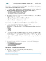
One-Period Stock Price as a Bernoulli Random Variable

Assumptions of the binomial distribution:
a) The probability of success (i.e. p) is constant for all
trials.
b) The trials are independent.
Bernoulli trial: A trial that generates one of two
outcomes is called a Bernoulli trial.
• In a Bernoulli trial with n number of trials, we can
have 0 to n successes.
• If the outcome of an individual trial is random, then
the total number of successes in n trials is also
random.
Binomial random variable X: It represents the number of
successes in n Bernoulli trials i.e.
X = sum of Bernoulli random variables
X = Y1 + Y2 + …+ Yn
where,
Yi = Outcome on the ith trial

Source: Example 2, Volume 1, Reading 10.


Number of sequences in n trials that result in x up moves
(or successes) and n – x down moves (or failures) is
calculated as follows:
݊!
ሺ݊ െ ‫ݔ‬ሻ! ‫!ݔ‬
where,
n! = n factorial = n(n - 1) (n - 2) ... 1 (and 0! = 1 by
convention).
Probability function for a binomial random variable:
݊
‫݌‬ሺ‫ݔ‬ሻ ൌ ܲሺܺ ൌ ‫ݔ‬ሻ ൌ ቀ ቁ ‫ ݌‬௫ ሺ1 െ ܲሻ௡ି௫
‫ݔ‬
݊!
ൌ
ሺ݊ െ ‫ݔ‬ሻ! ‫ ݌ !ݔ‬௫ ሺ1 െ ‫݌‬ሻ௡ି௫
for x = 0, 1, 2, …, n

• A binomial random variable is completely described
by two parameters i.e. n and p. It is stated as X~ B (n,
p)
read as “X has a binomial distribution with
parameters n and p”.
• Thus, a Bernoulli random variable is a binomial
random variable with n = 1 i.e. Y~B (1, p).

where,
x
=
n–x =

p
=
1–p=
n
=

# successes out of n trials
# failures out of n trials
probability of success
probability of failure
number of trials

Probability function of the Bernoulli random variable Y:
Probability of success:
• When the outcome is success Y = 1.
• When the outcome is failure Y = 0.
p (l) = P(Y= 1) = p = probability of success
p (0) = P( Y = 0) = 1 – p = probability of failure
For example, a stock price is a Bernoulli random variable
with probability of success (an up move) = p and
probability of failure (a down move) = 1 – p.
Suppose, Stock price today = S.
• When the stock price increases, ending price = uS =
(1 + rate of return if the stock moves up) × S
• When the stock price decreases, ending price = dS
1
ൌ
ൈ ܵ
1 ൅ ‫݌ݑݏ݁ݒ݋݉݇ܿ݋ݐݏ݄݁ݐ݂݅݊ݎݑݐ݁ݎ݂݋݁ݐܽݎ‬


1
P(X = 1) =   p1 (1− p)1−1 = p
1
Probability of failure:

1
P( X = 0) =   p 0 (1 − p )1−0 = 1 − p
0
NOTE:
When the probability of success on a trial is 0.50, the
binomial distribution is symmetric; otherwise, it is
asymmetric or skewed.


Reading 10

Common Probability Distributions

Example:

3.1

If a coin is tossed 20 times, what is the probability of
getting exactly 10 heads?
p
1–p
n
x

=

=
=
=

0.50
0.5
20
10

 
10
10
  (0.5) (0.5) = 0.176
10
 
20

Practice: Example 4, 5 & 6,
Volume 1, Reading 10.

Stock price movement on three consecutive days:
• Each day is an independent trial.
• When the stock moves up
u = 1 + rate of return for
an up move.
• When the stock moves down
d = 1 + rate of return
for a down move.

FinQuiz.com


Continuous Uniform Distribution

The continuous uniform distribution is the simplest
continuous probability distribution. The uniform
distribution has two main uses.
• It plays an important role in Monte Carlo simulation.
• It is an appropriate probability model to represent an
uncertainty in beliefs with equally likely outcomes.
Probability density function (pdf): It is used to assign the
probabilities to a continuous random variable and is
denoted as f (x). According to pdf,
• The probability that value of x lies between a and b
is the area under the graph of f(x) that lies between
a and b or the integral of f(x) over the range a to b.
 1
for a ≤ x ≤ b

f ( x) =  b − a

 0 elsewhere

• Over the range of values from a to b, density of the
ଵ
distribution of a random variable x =
.
ሺ௕ି௔ሻ

A binomial tree is shown below. Each boxed value that
represents successive moves (branch in the tree) is

called a node.

• Elsewhere, density of the distribution of a random
variable x = 0.

• In the fig below, a node reflects the potential value
for the stock price at a specified time.
• At each node, the transition probability for an up
move is p and for a down move is (1 – P).
Finding probability: The probabilities can be estimated
as follows:
‫ܨ‬ሺ‫ݔ‬ሻ ൌ

‫ݔ‬െܽ
݂‫ ܽݎ݋‬൏ ‫ ݔ‬൏ ܾ
ܾെܽ

• F (x) = area under the curve graphing the pdf.
• Under a Continuous uniform distribution, probabilities
for values of a continuous random variable x are
assigned across an interval of values of x; thus, the
probability that x takes on a specific value = 0.
• Since the probabilities at the endpoints a and b = 0
for any continuous random variable X, P (a ≤ X ≤ b)
= P (a < X ≤ b) = P (a ≤ X< b) = P (a< X < b).
• Each of the sequences uud, udu, and duu, has
probability = p2 (l – p).
• Stock price after three moves = P (S3 = uudS) = 3p2 (l p).
e.g. Number of ways to get 2 up moves in three periods
= 3! / (3 – 2)! 2! = 3


For a continuous uniform random variable:
Mean = µ = (a + b) / 2
Variance = σ2 = (b – a) 2 / 12
S.D. = √‫݁ܿ݊ܽ݅ݎܽݒ‬
• Note that S.D. is not a useful risk measure for a
uniform distribution; rather, the S.D. is a good risk
measure for Normal Distribution.


Reading 10

Common Probability Distributions

Example:

FinQuiz.com

• The smaller the S.D., the more the observations are
concentrated around the mean.

Suppose,
At the lower bound = a =100,000 km
total cost
= $40,000.
At the upper bound = b =150,000 km
total cost
= $60,000.
Outside the lower and upper bound
total cost = $0.

x = total anticipated annual travel costs in thousands of
dollars
• Over the range of values from $40,000 to $60,000,
the distribution has density f(x) = 1/ (60 - 40) = 1/20.
• Elsewhere, the distribution has density f(x) = 0.

The probability that travel costs are between 40 and 60 =
Total area under the density function f(x) between 40
and 60 = height × length (or base) = (1/20) × (60–40) = 1
The probability that travel costs are between 40 and 50 =
Area under the curve between 40 & 50 = (1/20) × (50–40)
= 0.50

Practice: Example 7,
Volume 1, Reading 10.

3.2

The Normal Distribution

• A normal distribution is a distribution that is symmetric
about the centre (mean) and is bell-shaped. Thus,
o Mean = median = mode.
o Skewness = 0.
o Kurtosis = 3 and Excess kurtosis = 0.
• The range of possible outcomes of the normal
distribution is the entire real line i.e. all real numbers
lying between -∞ and +∞.
• The tails of the normal distribution never touches the
horizontal axis and extend without limit to the left

and to the right; however, as we move away from
the center, the tails get closer and closer to the
horizontal axis. This characteristic is referred to as the
distribution is asymptotic to the horizontal axis.
• The normal distribution is described by two
parameters i.e. its mean (µ) and its variance (σ2) or
standard deviation (σ). It is stated as:
X ~ N (µ, σ2)
read “X follows a normal distribution
with mean µ and variance σ2”.
o When the mean increases (decreases), the curve
shifts to the right (left).
• When the standard deviation increases (decreases),
the curve flattens (steepens).

• Since the normal distribution is symmetrical, it tends
to underestimate the probability of extreme returns.
Thus, it is not appropriate to use for Options.
• The normal distribution can be used to model
returns; however, is not appropriate to use to model
asset prices.
• According to the central limit theorem, sum and
mean of a large number of independent random
variables is approximately normally distributed.
• It is important to note that a linear combination of
two or more normal random variables is also
normally distributed.
A univariate normal distribution describes the probability
of a single random variable.
A multivariate normal distribution describes the

probabilities for a group of related random variables. It is
completely defined by three parameters:
1. The list of the mean returns on the individual
securities i.e. total means = n.
2. The list of the securities’ variances of return i.e. total
variances = n.
3. The list of all the distinct pair-wise return correlations
i.e. total distinct correlations = n (n - 1) / 2.
For example, a bivariate normal distribution (i.e. a
distribution with 2 stocks) has:
• Means = 2
• Variances = 2
• Correlation = 2 (2 –1) / 2 = 1
For a normal random variable standard deviation of:
• Sample skewness = 6/ n
• Sample kurtosis = 24/ n
Normal density function: It is expressed as follows:
݂ሺ‫ݔ‬ሻ =

1

ߪ√2ߨ

݁‫ ݌ݔ‬ቆ

−(‫ ݔ‬− ߤ)ଶ
ቇ for − ∞ < ‫ < ݔ‬+∞
2ߪ ଶ

• The probability that a normally distributed variable x

takes on values in the range from a to b = Area
under f(x) between a and b.


Reading 10

Common Probability Distributions

• The total area under the curve = 1.
• The area under the curve to the left of centre = 0.5
and the area right of centre = 0.5.
o Approximately 50% of all observations fall in the
interval µ ± (2/ 3) σ.
o Approximately 68% of all observations fall in the
interval µ ± σ.
o Approximately 95% of all observations fall in the
interval µ ± 2σ.
o Approximately 99% of all observations fall in the
interval µ ± 3σ.
• More-precise intervals are µ ± 1.96σ for 95% of the
observations and µ ± 2.58σ for 99% of the
observations.

FinQuiz.com

Example:
• Finding P (Z > 1.23):

• Finding P (-0.75 < Z < 1.23):


Standard normal distribution or unit normal distribution: It
is a normal distribution with:
• The mean (µ ) = 0
• Standard deviation (σ) =1
When X is normally distributed, it can be standardized
using the following formula:
Z=

• Finding P (Z< -2.33):

ࢄିࣆ
࣌

• Z –score indicates how many standard deviations
away from the mean the point x lies.
Example:

Example:

Suppose, a normal random variable, X = 9.5 with µ = 5
and σ = 1.5.
Z = (9.5 - 5) / 1.5 = 3
Example:
Finding the Probability i.e. P (Z < 2.67). It is found by first
finding 2.6 in the left hand column, and then moving
across the row to the column under 0.07. (Refer to table
on the next page). Thus,

The average (µ) on a corporate finance test was 78 with
a standard deviation of 8 (σ). If the test scores are

normally distributed, find the probability that a student
receives a test score greater than 85.
Z=

଼ହି଻଼
଼

= 0.875 ≈ 0.88

The area to the left of z = 2.67 = 0.9962.
• In order to find the area to the right of z, we use the
Standard Normal Table given below to find the area
that corresponds to z-value and then subtract the
area from 1.
• Probability to the right of x = 1.0 - N(x).
• Since the normal distribution is symmetric around its
mean, the area and the probability to the right of x =
area and the probability to the left of -x, N (-x).
• The probability to the right of –x i.e. P (Z ≥ -x) = N(x).

P(x> 85) = P (z> 0.88) = 1 −P(z< 0.88) = 1 − 0.8106
= 0.1894 .


Reading 10

Common Probability Distributions

FinQuiz.com


NOTE:
• P (Z ≤ 1.282) = 0.90 = 90% → It implies that 90th
percentile point = 1.282 and % of values in the right
tail = 10%.
• P (Z ≤ 1.65) = 0.95 = 95% → It implies that the 95th
percentile point = 1.65 and % of values in the right
tail = 5%.
• P (Z ≤ 2.327) = 0.99 = 99% → It implies that the 99th
percentile point = 2.327 and % of values in the right
tail = 1%.

Practice: Example 8,
Volume 1, Reading 10.

3.3

Applications of the Normal Distribution

• The mean-variance analysis is based on the
assumption that returns are normally distributed.
• Safety-first rule: Safety-first rule focuses on shortfall
risk i.e. the risk that portfolio value will fall below
some minimum acceptable level over some
specified time horizon. For example, the risk that the
assets in a defined benefit plan will fall below plan
liabilities.
According to Roy's safety-first criterion, the optimal
portfolio is the one that minimizes the probability that
portfolio return (Rp) falls below the threshold level (RL).
When returns are normally distributed, the safety-first

optimal portfolio is the portfolio that maximizes the
safety-first ratio (SFRatio):
ܵ‫ = ݋݅ݐܴܽܨ‬ሾ‫ܧ‬ሺܴ௉ ሻ − ܴ௅ ሿ/ߪ௉
• Investors prefer the portfolio with the highest SFRatio.
• Probability that the portfolio return < threshold level =
P (Rp< RL) = N (-SFRatio).
• The optimal portfolio has the lowest P (Rp< RL).
Example:
•
•
•
•

Portfolio 1 expected return = 12% and S.D. = 15%
Portfolio 2 expected return = 14% and S.D. = 16%
Threshold level = 2%
Assumes that returns are normally distributed.
SFRatio of portfolio 1 = (12 – 2) / 15 = 0.667
SFRatio of portfolio 2 = (14 – 2) / 16 = 0.75

• Since SFRatio of portfolio 2 > SFRatio 1, the superior
Portfolio is Portfolio 2.


Reading 10

Common Probability Distributions

Probability that return < 2% = N (–0.75) = 1 – N (0.75)
= 1 – 0.7734*

≈ 23%.
*Refer to table on previous page.
Sharpe Ratio:
Sharpe ratio = [E (Rp) – Rf] / σp
• The portfolio with the highest Sharpe ratio is the one
that minimizes the probability that portfolio return will
be less than the risk-free rate (assuming returns are
normally distributed).

Practice: Example 9,
Volume 1, Reading 10.

Managing Financial risk: Two important measures used
to manage financial risk include:

FinQuiz.com

given that Y is lognormal.
Mean (µL) of a lognormal random variable =
exp (µ + 0.50σ2)
Variance (σL2) of a lognormal random variable
= exp (2µ+ σ2) × [exp (σ2) – 1].
Strengths of lognormal distribution:
• The lognormal distribution is more appropriate
(relative to normal distribution) to use to model asset
prices because asset prices cannot be negative.
• It is used in Black-Scholes-Merton model, which
assumes that the asset’s price underlying the option
is lognormally distributed.
It is important to note that when a stock's continuously

compounded return is normally distributed, then future
stock price is necessarily lognormally distributed.
ST = S0exp (r0,T)

• Value at risk (VAR): It provides the minimum value of
losses (in money terms) expected over a specified
time period (e.g. a day, quarter, year etc.) at a
specified level of probability (e.g. 5%, 1%). VAR
estimated using variance-covariance or analytical
method assumes that returns are normally
distributed.
Example:
A one week VAR of $10 million for a portfolio with 5%
probability implies that portfolio is expected to loss
$10 million or more in a single week.
• Stress testing/scenario analysis: It involves a use of
set of techniques to estimate losses in extremely
worst combinations of events or scenarios.
3.4

The Lognormal Distribution

A random variable (i.e. Y) whose natural logarithm (i.e. ln
Y) has a normal distribution, is said to have a Lognormal
distribution.

Where,
exp = e
r0,t = Continuously compounded return from 0 to T
• Since ST is proportional to the log of a normal

random variable → ST is lognormal.
Price relative = Ending price / Beginning price =
St+1/ St=1 + Rt, t+1
where,
Rt, t+1 = holding period return on the stock from t to t + 1.
Continuously compounded return associated with a
holding period from t to t + 1:
rt, t+1= ln(1 + holding period return)
Or
rt, t+1 = ln(price relative) = ln (St+1 / St) = ln (1 + Rt,t+1)
NOTE:

• Unlike Normal distribution, Lognormal random
variables cannot be negative.
Reason:
Since, negative values do not have logarithms, Y is
always > 0 and thus the distribution is positively skewed
(unlike normal distribution that is bell-shaped).

The continuously compounded return < associated
holding period return.
Continuously compounded return associated with a
holding period from 0 to T:
R0,T= ln (ST / S0)
Or
‫ݎ‬଴,் = ‫ି்ݎ‬ଵ,் + ‫ି்ݎ‬ଶ,்ିଵ + ⋯ + ‫ݎ‬଴,ଵ
Where,
rT-I, T = One-period continuously compounded returns

• Like normal distribution, it is completely described by

two parameters i.e. the mean and variance of In Y,


Reading 10

Common Probability Distributions

FinQuiz.com

Example:

Volatility:

Suppose, one-week holding period return = 0.04.

Volatility reflects the deviation of the continuously
compounded returns on the underlying asset around its
mean. It is estimated using a historical series of
continuously compounded daily returns.

Equivalent continuously compounded return =
one-week continuously compounded return = ln (1.04)
= 0.039221
• The intervals within which a certain percentage of
the observations of a normally distributed random
variable are expected to lie are symmetric around
the mean.
• The intervals within which a certain percentage of
the observations of a lognormally distributed
random variable are expected to lie are not

symmetric around the mean.

Annualized volatility = sample S.D. of one period
continuously compounded returns
× √ܶ
where,
T = Number of trading days in a year = 250.
Example:
Michelin Daily Closing Prices

In many investment applications, it is assumed that
returns are independently and identically distributed
(IID).
• Returns are independently distributed implies that
investors cannot forecast future returns using past
returns (i.e., weak-form market efficiency).
• Returns are identically distributed implies that the
mean and variance of return do not change from
period to period (i.e. stationarity).
When one-period continuously compounded returns (i.e.
r0,1) are IID random variables with mean µ and variance
σ2, then
‫ܧ‬൫‫ݎ‬଴,் ൯ = ‫ܧ‬൫‫ି்ݎ‬ଵ,் ൯ + ‫ܧ‬൫‫ି்ݎ‬ଶ,்ିଵ ൯ + ⋯ + ‫ܧ‬൫‫ݎ‬଴,ଵ ൯ = ߤܶ
And
ܸܽ‫ ߪ = ݁ܿ݊ܽ݅ݎ‬ଶ ൫‫ݎ‬଴,் ൯ = ߪ ଶ ܶ

Closing Price (€)

31 March


25.20

01 April

25.21

03 April

25.52

03 April

26.10

04 April

26.14

Since, rt, t+1 = ln (St+1 / St) = ln (1 + Rt,t+1)
•
•
•
•

ln (25.21 / 25.20) = 0.000397
ln (25.52 / 25.21) = 0.012222
ln (26.10 / 25.52) = 0.022473
ln (26.14 / 26.10) = 0.001531

Sum = 0.036623

Mean = 0.009156
Variance = 0.000107
S.D. = 0.010354

S.D. = σ (r0,T) = σ√ܶ
• It implies that when the one-period continuously
compounded returns are normally distributed, then
the T holding period continuously compounded
return (i.e. r0,T) is also normally distributed with mean
µT and variance σ2T.
• According to Central limit theorem, the sum of oneperiod continuously compounded returns is
approximately normal even if they are not normally
distributed.
4.

Date (2003)

Annualized volatility = 0.010354 × √250 = 0.163711
Expected continuously compounded annual return
= Sample mean × T
= 0.009156 (250)
= 2.289
Source: Example 10, Volume 1, Reading 10.

MONTE CARLO SIMULATION

Monte Carlo simulation involves the use of a computer
to generate a large number of random samples from a
probability distribution. It can be used in conjunction
with (i.e. as a complement) analytical methods.

Uses:
• It is used in planning and managing financial risk.
• It can be used in valuing complex securities e.g.
European-style options, mortgage-backed securities.

• It can be used to estimate VAR e.g. using Monte
Carlo simulation, portfolio's profit and loss
performance for a specified time horizon are
simulated to generate a frequency distribution for
changes in portfolio value; the point that reflects the
end point of the least favorable 5% of simulated
changes is 95% VAR.
• It can be used to examine a model's sensitivity to
changes in the assumptions.


Reading 10

Common Probability Distributions

Advantages: Monte Carlo simulation can be used to
value complex securities i.e. European-style
options.

FinQuiz.com

8) This process is repeated until a specified number of
trials, i, is completed (e.g. tens of thousands of trials).
NOTE:


Drawbacks: Unlike analytical methods (e.g. BlackScholes-Merton option pricing model),
Monte Carlo simulation provides only
statistical estimates, not exact results. In
addition, unlike black-scholes model,
Monte Carlo simulation model cannot be
used to quickly measure the sensitivity of
call option value to changes in current
stock price and other variables.
Steps of Monte Carlo simulation technique to examine a
model's sensitivity to changes in assumptions:
1) Specify the underlying variable or variables e.g. stock
price for an equity call option.
2) Specify the beginning values of the underlying
variables e.g. stock price.
• C iT = Value of the option at maturity T. The subscript I
reflects a value resulting from the ith simulation trial.
3) Specify a time period.
Time increment = ∆t
= Calendar time / Number of subperiods (K)
4) Specify the regression model for changes in stock
price.
∆ሺܵ‫݁ܿ݅ݎ݌݇ܿ݋ݐ‬ሻ ൌ ሺߤ ൈ ܲ‫ ݁ܿ݅ݎ݌݇ܿ݋ݐݏݎ݋݅ݎ‬ൈ ∆‫ݐ‬ሻ ൅ ሺߪ
ൈ ܲ‫ ݁ܿ݅ݎ݌݇ܿ݋ݐݏݎ݋݅ݎ‬ൈ ܼ௞ ሻ
where,
Zk= Risk factor in the simulation. It is a standard normal
random variable.
5) K random variables are drawn for each risk factor
using a computer program or spreadsheet function.
6) Now the underlying variables are estimated by
substituting values of random observations in the

model specified in Step 4.
7) The value of a call option at maturity i.e. CiT is
calculated and then this value is discounted back at
time period 0 to get Ci0.

For obtaining each extra digit of accuracy in results, the
appropriate increase in the number of trials depends on
the problem. For example, in option value, tens of
thousands of trials may be appropriate. Generally, the
number of trials should be increased by a factor of 100.
9) Finally, mean value and S.D. for the simulation are
calculated.
Mean value = Average value of the option over all trials
in the simulation
• The mean value will be the Monte Carlo estimate of
the value of the call option.
Random number generator: An algorithm that generates
uniformly distributed random numbers between 0 and 1
is referred to as random number generator. It is
important to note that random observations from any
distribution can be generated using a uniform random
variable.
Steps to generate random observations on variable X:
1) Generate a uniform random number (i.e. T) between
0 and 1 using the random number generator.
2) Evaluate the inverse of cumulative distribution
function F(x) i.e. F-1 (x) to obtain a random
observation on variable X.
Historical simulation or Back simulation: Under a
historical simulation, samples are generated using a

historical record of underlying variables to simulate a
process. It is based on the assumption that historical
data can be used to predict future.
Drawback of Historical simulation: Unlike Monte Carlo
simulation, historical simulation cannot be used to
perform “what if” analyses.

Practice: Example 11 & 12,
Volume 1, Reading 10 & End of
Chapter Practice Problems for
Reading 10.