Power systems analysis 2nd edition by hadi saadat

Bạn đang xem bản rút gọn của tài liệu. Xem và tải ngay bản đầy đủ của tài liệu tại đây (1.46 MB, 285 trang )

www.EngineeringBooksPdf.com

Solutions Manual

Hadi Saadat
Professor of Electrical Engineering
Milwaukee School of Engineering
Milwaukee, Wisconsin

McGraw-Hill, Inc.

www.EngineeringBooksPdf.com

CONTENTS

1

THE POWER SYSTEM: AN OVERVIEW

1

2

BASIC PRINCIPLES

5

3

GENERATOR AND TRANSFORMER MODELS;
THE PER-UNIT SYSTEM

25

4

TRANSMISSION LINE PARAMETERS

52

5

LINE MODEL AND PERFORMANCE

68

6

POWER FLOW ANALYSIS

107

7

OPTIMAL DISPATCH OF GENERATION

147

8

SYNCHRONOUS MACHINE TRANSIENT ANALYSIS

170

9

BALANCED FAULT

181

10 SYMMETRICAL COMPONENTS AND UNBALANCED FAULT

208

11 STABILITY

244

12 POWER SYSTEM CONTROL

263

i

www.EngineeringBooksPdf.com

CHAPTER 1 PROBLEMS

1.1 The demand estimation is the starting point for planning the future electric
power supply. The consistency of demand growth over the years has led to numerous attempts to fit mathematical curves to this trend. One of the simplest curves
is
P = P0 ea(t−t0 )
where a is the average per unit growth rate, P is the demand in year t, and P0 is
the given demand at year t0 .
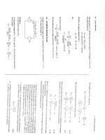
Assume the peak power demand in the United States in 1984 is 480 GW with
an average growth rate of 3.4 percent. Using MATLAB, plot the predicated peak
demand in GW from 1984 to 1999. Estimate the peak power demand for the year
1999.
We use the following commands to plot the demand growth
t0 = 84; P0 = 480;
a =.034;
t =(84:1:99)’;
P =P0*exp(a*(t-t0));
disp(’Predicted Peak Demand - GW’)
disp([t, P])
plot(t, P), grid
xlabel(’Year’), ylabel(’Peak power demand GW’)
P99 =P0*exp(a*(99 - t0))

The result is
1

www.EngineeringBooksPdf.com

2

CONTENTS

Predicted Peak Demand - GW
84.0000 480.0000
85.0000 496.6006
86.0000 513.7753
87.0000 531.5441
88.0000 549.9273
89.0000 568.9463
90.0000 588.6231
91.0000 608.9804
92.0000 630.0418
93.0000 651.8315
94.0000 674.3740
95.0000 697.6978
96.0000 721.8274
97.0000 746.7916
98.0000 772.6190
99.0000 799.3398
P99 =
799.3398
The plot of the predicated demand is shown n Figure 1.
800 . . . . . . . ... . . . . . . ... . . . . . . ... . . . . . . ... . . . . . . ... . . . . . . ... . . . . . . ... . . . . . . ..
.
.

.
.

.
.

.
.

.
.

.
.

.....
...... .
......

.
.

750 . . . . . . . .. . . . . . . ... . . . . . . ... . . . . . . ... . . . . . . ... . . . . . . ... ............................ . . ... . . . . . . ..
700
Peak
650
Power
Demand 600
GW
550
500

.
.
.

.
.
.......
......
.
.
.
.
.
...... .
......
. . . . . . . .. . . . . . . .. . . . . . . .. . . . . . . .. . . . . . . .. . . .............. . . .. .
.
.
.
.
.
. .......
.
.
.
.
.
. ......
.
.......
.
.
.
.

.
........
...... .
.
.
.
.
.
.
.
.
.
.
.
. . . . . . . .. . . . . . . .. . . . . . . .. . . . . . . .. . ............... . . .. . . . . . . .. .
..
.
.
.
.
.
.
.
.
.........
.
.
.
.
.....

.
.
.
.
.
....... .
.......
.
.
.
.
.
.
.......
.
.
.
.
.
.
. . . . . . . . . . . . . . .. . . . . . . .. ........ . . . . .. . . . . . . .. . . . . . . .. .
.
.
.
.
.
.
.
.
.

....
.
.
.
.
.
.
.
..... .
.
.
.
.
.
........
.
. ..............
.
.
.
.
.
.
.
.
.
.
.
. . . . . . . .. . . . . . .............. . . . . . . .. . . . . . . .. . . . . . . .. . . . . . . .. .
.

.
.
.
.
.... .
.
.
.
.
.
.
.
......
.
.
.
.
.
.
........
. .......
.
.
.
.
.
.........
.
.
.

.
.
.
.
.
.
.
.
.
..
. . . .................. . .. . . . . . . .. . . . . . . .. . . . . . . .. . . . . . . .. . . . . . . .. .
.
.
.
.
.
.
.
....
.
.
.
.
.
.
.........
.
.
.
.

.
.
.
.
.
.
.
.
. . . . . . . . . . . . . . .. . . . . . . .. . . . . . . .. . . . . . . .. . . . . . . .. .

450
84

86

88

90

92

94

96

.
.
. . . . . ..
.
.

.
.
. . . . . ..
.
.
.
. . . . . ..
.
.
.
. . . . . ..
.
.
.
.
. . . . . ..
.
.
.
. . . . . ..

98

.
.
. . . . . ..
.
.
.
.

. . . . . ..
.
.
.
. . . . . ..
.
.
.
. . . . . ..
.
.
.
.
. . . . . ..
.
.
.
. . . . . ..

100

Year
FIGURE 1
Peak Power Demand for Problem 1.1

1.2 In a certain country, the energy consumption is expected to double in 10 years.

www.EngineeringBooksPdf.com

CONTENTS

3

Assuming a simple exponential growth given by
P = P0 eat
calculate the growth rate a.
2P0 = P0 e10a
ln 2 = 10a
Solving for a, we have
a =

0.693
= 0.0693 = 6.93%
10

1.3. The annual load of a substation is given in the following table. During each
month, the power is assumed constant at an average value. Using MATLAB and
the barcycle function, obtain a plot of the annual load curve. Write the necessary
statements to find the average load and the annual load factor.
Annual System Load
Interval – Month Load – MW
January
8
February
6
March
4
April
2

May
6
June
12
July
16
August
14
September
10
October
4
November
6
December
8
The following commands
data = [ 0
1
2
3
4
5

1
2
3
4
5
6

8
6
4
2
6
12

www.EngineeringBooksPdf.com

4

CONTENTS

6
7
16
7
8
14
8
9
10
9 10
4
10 11
6
11 12
8];

P = data(:,3);
% Column array of load
Dt = data(:, 2) - data(:,1); % Column array of demand interval
W = P’*Dt;
% Total energy, area under the curve
Pavg = W/sum(Dt)
% Average load
Peak = max(P)
% Peak load
LF = Pavg/Peak*100
% Percent load factor
barcycle(data)
% Plots the load cycle
xlabel(’time, month’), ylabel(’P, MW’), grid
result in
Pavg =
8
Peak =
16
LF =
50

16
14
12
10
P
MW

8

6
4
2
0

.
.
...................................
.
.
...
...
.
.
.
.
...
...
...
.
.
.
.
..
.
..
.
.
.
.

.....
.
.
.
.
.
.
.
..
.
...
....
.
.
.
.
.
.
. . . . . . . . . . . . . . . . . . . . . . . . . ... . . . . . . . . . . . . . .................................. . . . . .. . . . . . . . . .
.
.
.
.
.
...
..
...
...
.
.

.
.
...
.
.
. . . . . . . . . . .. . . . . ................................... . . . . . . . . . . . . . . . . . . . .. . . . . . . . . . .. . . . . . . . . .
.
.
.
.
.
.
.
.
.
.
.
.
.
.
.
.
.
.
.
.

0

2

4

6

8

10

12

time, month
FIGURE 2
Monthly load cycle for Problem 1.3

www.EngineeringBooksPdf.com

CHAPTER 2 PROBLEMS

2.1. Modify the program in Example 2.1 such that the following quantities can be
entered by the user:
The peak amplitude Vm , and the phase angle θv of the sinusoidal supply v(t) =
Vm cos(ωt + θv ). The impedance magnitude Z, and its phase angle γ of the load.
The program should produce plots for i(t), v(t), p(t), pr (t) and px (t), similar to
Example 2.1. Run the program for Vm = 100 V, θv = 0 and the following loads:
An inductive load, Z = 1.25 60◦ Ω
A capacitive load, Z = 2.0 −30◦ Ω
A resistive load, Z = 2.5 0◦ Ω
(a) From pr (t) and px (t) plots, estimate the real and reactive power for each load.

Draw a conclusion regarding the sign of reactive power for inductive and capacitive loads.
(b) Using phasor values of current and voltage, calculate the real and reactive power
for each load and compare with the results obtained from the curves.
(c) If the above loads are all connected across the same power supply, determine
the total real and reactive power taken from the supply.
The following statements are used to plot the instantaneous voltage, current, and
the instantaneous terms given by(2-6) and (2-8).
Vm = input(’Enter voltage peak amplitude Vm = ’);
thetav =input(’Enter voltage phase angle in degree thetav = ’);
Vm = 100; thetav = 0;
% Voltage amplitude and phase angle
Z = input(’Enter magnitude of the load impedance Z = ’);
gama = input(’Enter load phase angle in degree gama = ’);
thetai = thetav - gama;
% Current phase angle in degree
5

www.EngineeringBooksPdf.com

6

CONTENTS

theta = (thetav - thetai)*pi/180;
% Degree to radian
Im = Vm/Z;
% Current amplitude
wt=0:.05:2*pi;
% wt from 0 to 2*pi

v=Vm*cos(wt);
% Instantaneous voltage
i=Im*cos(wt + thetai*pi/180);
% Instantaneous current
p=v.*i;
% Instantaneous power
V=Vm/sqrt(2); I=Im/sqrt(2);
% RMS voltage and current
pr = V*I*cos(theta)*(1 + cos(2*wt));
% Eq. (2.6)
px = V*I*sin(theta)*sin(2*wt);
% Eq. (2.8)
disp(’(a) Estimate from the plots’)
P = max(pr)/2, Q = V*I*sin(theta)*sin(2*pi/4)
P = P*ones(1, length(wt));
% Average power for plot
xline = zeros(1, length(wt));
% generates a zero vector
wt=180/pi*wt;
% converting radian to degree
subplot(221), plot(wt, v, wt, i,wt, xline), grid
title([’v(t)=Vm coswt, i(t)=Im cos(wt +’,num2str(thetai),’)’])
xlabel(’wt, degrees’)
subplot(222), plot(wt, p, wt, xline), grid
title(’p(t)=v(t) i(t)’), xlabel(’wt, degrees’)
subplot(223), plot(wt, pr, wt, P, wt,xline), grid
title(’pr(t)
Eq. 2.6’), xlabel(’wt, degrees’)
subplot(224), plot(wt, px, wt, xline), grid
title(’px(t) Eq. 2.8’), xlabel(’wt, degrees’)

subplot(111)
disp(’(b) From P and Q formulas using phasor values ’)
P=V*I*cos(theta)
% Average power
Q = V*I*sin(theta)
% Reactive power
The result for the inductive load Z = 1.25 60◦ Ω is
Enter
Enter
Enter
Enter

voltage peak amplitude Vm = 100
voltage phase angle in degree thatav = 0
magnitude of the load impedance Z = 1.25
load phase angle in degree gama = 60

(a) Estimate from the plots
P =
2000
Q =
3464
(b) For the inductive load Z = 1.25 60◦ Ω, the rms values of voltage and current
are
100 0◦
V =
= 70.71 0◦ V
1.414

www.EngineeringBooksPdf.com

CONTENTS

v(t) = Vm cos ωt, i(t) = Im cos(ωt − 60)
6000
......
100 ................
....
....
50
0
−50
−100

4000
3000
2000
1000
0

... ........
..
...
......... ..........
..... ..
...
....
....
.... .....

..
.
.
.
...
.
...
...
...
...
...
...
...
...
...
...
.
...
...
...
..
...
.
...
...
..
...
..
...
..

.
...
...
...
...
...
..
...
...
...
..
...
...
...
.... ....
...
...
.
.
.
.
.
.
......
...
....
...
..................
....
...

.....
....
................

0

100

200

300

2000
0

p(t) = v(t)i(t)
........
.........
... .....
... ....
...
...
...
...
...
...
....
....
...
...

.
.
..
..
...
...
.
.
.
.
...
...
..
...
.
...
...
.
.
.
...
...
.
.
..
...
.
...
.
.

...
...
.
...
...
...
...
....
...
..
...
.
...
...
...
..
...
...
...
...
...
...
...
..
...
...
..
...
.
..

... .....
... ....
... ..
... ..
........
......

−2000
400
0

100

200

300

ωt, degrees

ωt, degrees

pr (t), Eq. 2.6

px (t), Eq. 2.8

.....
.........
..
...
... ....

...
...
...
...
...
...
...
..
....
...
.
...
...
..
...
...
...
...
...
...
..
...
...
...
..
...
.
..
.
.

...
...
...
...
..
..
...
...
..
..
.
.
.
.
...
...
...
...
...
...
...
...
...
...
...
...
...
...
...
...

....
....
...
.
...
..
..
...
...
..
... .....
... ....
.... ...
..........
..

0

4000

100

200

300

4000
2000
0
−2000

400

...........
...........
... ....
... .....
...
...
...
...
...
..
..
...
.
.
...
...
...
...
...
...
..
.
....
...
...
..
...

...
...
..
...
...
...
..
..
.
.
...
...
..
..
.
...
.
.
.
...
...
...
...
...
...
...
...
...
...
..

..
...
..
..
...
.
.
.
.
.
.
.... ...
.... ....
......
.....

−4000
400
0

ωt - degrees

7

100

200

300

400

ωt, degrees

FIGURE 3
Instantaneous current, voltage, power, Eqs. 2.6 and 2.8.

I=

70.71 0◦
= 56.57 −60◦ A
1.25 60◦

Using (2.7) and (2.9), we have
P = (70.71)(56.57) cos(60) = 2000 W
Q = (70.71)(56.57) sin(60) = 3464 Var
Running the above program for the capacitive load Z = 2.0 −30◦ Ω will result in
(a) Estimate from the plots
P =
2165
Q =
-1250

www.EngineeringBooksPdf.com

8

CONTENTS

Similarly, for Z = 2.5 0◦ Ω, we get
P =
2000
Q =
0
(c) With the above three loads connected in parallel across the supply, the total real
and reactive powers are
P = 2000 + 2165 + 2000 = 6165 W
Q = 3464 − 1250 + 0 = 2214 Var
2.2. A single-phase load is supplied with a sinusoidal voltage
v(t) = 200 cos(377t)
The resulting instantaneous power is
p(t) = 800 + 1000 cos(754t − 36.87◦ )
(a) Find the complex power supplied to the load.
(b) Find the instantaneous current i(t) and the rms value of the current supplied to
the load.
(c) Find the load impedance.
(d) Use MATLAB to plot v(t), p(t), and i(t) = p(t)/v(t) over a range of 0 to 16.67
ms in steps of 0.1 ms. From the current plot, estimate the peak amplitude, phase
angle and the angular frequency of the current, and verify the results obtained in
part (b). Note in MATLAB the command for array or element-by-element division
is ./.
p(t) = 800 + 1000 cos(754t − 36.87◦ )
= 800 + 1000 cos 36.87◦ cos 754t + sin 36.87◦ sin 754t
= 800 + 800 cos 754t + 600 sin 754t
= 800[1 + cos 2(377)t] + 600 sin 2(377)t
p(t) is in the same form as (2.5), thus P = 600 W, and Q = 600, Var, or
S = 800 + j600 = 1000 36.87◦ VA
(b) Using S = 12 Vm Im ∗ , we have
1

1000 36.87◦ = 200 0◦ Im
2

www.EngineeringBooksPdf.com

CONTENTS

or
Im = 10 −36.87◦ A
Therefore, the instantaneous current is
i(t) = 10cos(377t − 36.87◦ ) A
(c)
ZL =

V
200 0◦
=
= 20 36.87◦ Ω
I
10 −36.87◦

(d) We use the following command
v(t)

p(t)

200 .................

2000

100

1500

0
−100
−200

0

......
....
....
...
...
...
..
...
.
...
...
...
..
..
..
..
..
..
..

.
..
..
..
..
..
..
..
...
...
..
...
.
...
...
...
...
..
..
..
..
..
.
..
..
..
..
..
..
...

..
...
..
.
.
...
...
...
..
...
...
...
....
...
.
.
.
...... .....
........

100

200

300

1000
500
0
400

−500

.......
......
... .....
... .....
..
..
...
...
..
...
...
...
.
..
.
...
.
..
...
.
...
.
..
...
.
.
..

..
..
.
.
...
..
..
.
.
.
.
.
.
...
...
...
...
...
...
...
...
...
...
..
...
...
...
..
..
...

.
.
.
.
...
...
...
...
...
..
..
..
..
..
..
..
...
...
..
..
...
..
...
.
....
..
..
...
..
...

..
...
..
...
..
... ....
... ....
........
........
.

0

100

200

300

ωt, degrees

ωt, degrees
i(t)
10
5
0
−5
−10

................

.....
....
...
...
...
...
..
..
..
..
...
..
...
..
.
.
...
...
...
..
..
..
..
..
..
..
..
.
.
..

..
..
..
..
..
..
..
..
..
..
.
.
..
..
...
...
...
..
...
..
...
.
.
.
..
..
...
..
...
...

...
...
....
.
.
.
.
.....
................

0

100

200

300

400

ωt, degrees
FIGURE 4
Instantaneous voltage, power, and current for Problem 2.2.

www.EngineeringBooksPdf.com

400

9

10

CONTENTS

Vm = 200;
t=0:.0001:0.01667;
% wt from 0 to 2*pi
v=Vm*cos(377*t);
% Instantaneous voltage
p = 800 + 1000*cos(754*t - 36.87*pi/180);% Instantaneous power
i=p./v;
% Instantaneous current
wt=180/pi*377*t;
% converting radian to degree
xline = zeros(1, length(wt));
% generates a zero vector
subplot(221), plot(wt, v, wt, xline), grid
xlabel(’wt, degrees’), title(’v(t)’)
subplot(222), plot(wt, p, wt, xline), grid
xlabel(’wt, degrees’), title(’p(t)’)
subplot(223), plot(wt, i, wt, xline), grid
xlabel(’wt, degrees’), title(’i(t)’), subplot(111)
The result is shown in Figure 4. The inspection of current plot shows that the peak
amplitude of the current is 10 A, lagging voltage by 36.87◦ , with an angular frequency of 377 Rad/sec.
2.3. An inductive load consisting of R and X in series feeding from a 2400-V rms
supply absorbs 288 kW at a lagging power factor of 0.8. Determine R and X.
◦
+

R

I

X

.......... ..... ...... ...... ...... .......................................................
.... ..... ..... ....
..

◦
−

V

FIGURE 5
An inductive load, with R and X in series.

θ = cos−1 0.8 = 36.87◦
The complex power is
S=

288
36.87◦ = 360 36.87◦ kVA
0.8

The current given from S = V I ∗ , is
I=

360 × 103 −36.87◦

= 150 −36.87 A
2400 0◦

Therefore, the series impedance is
Z = R + jX =

V
2400 0◦
= 12.8 + j9.6 Ω
=
I
150 −36.87◦

Therefore, R = 12.8 Ω and X = 9.6 Ω.

www.EngineeringBooksPdf.com

CONTENTS

11

2.4. An inductive load consisting of R and X in parallel feeding from a 2400-V
rms supply absorbs 288 kW at a lagging power factor of 0.8. Determine R and X.
◦

.
..........
..
.

....................................
...
...
...
...
.....
.
..........
.
........
..
.
.
.
.
.
.......
.
.......
.
.
.
............
.
.......
...
............
..
.......
.....

..
...
...
....
..
.................................
...
...

I
+

R

V

X

−
◦

FIGURE 6
An inductive load, with R and X in parallel.

The complex power is
S=

288
36.87◦ = 360 36.87◦ kVA
0.8

= 288 kW + j216 kvar

|V |2
(2400)2
=
= 20 Ω
P
288 × 103
(2400)2
|V |2
=
= 26.667 Ω
X=
Q
216 × 103
R=

2.5. Two loads connected in parallel are supplied from a single-phase 240-V rms
source. The two loads draw a total real power of 400 kW at a power factor of 0.8
lagging. One of the loads draws 120 kW at a power factor of 0.96 leading. Find the
complex power of the other load.
θ = cos−1 0.8 = 36.87◦
The total complex load is
S=

400
36.87◦ = 500 36.87◦ kVA
0.8
= 400 kW + j300 kvar

The 120 kW load complex power is
S=

120
−16.26◦ = 125 −16.26◦ kVA
0.96
= 120 kW − j35 kvar

www.EngineeringBooksPdf.com

12

CONTENTS

Therefore, the second load complex power is
S2 = 400 + j300 − (120 − j35) = 280 kW + j335 kvar
2.6. The load shown in Figure 7 consists of a resistance R in parallel with a capacitor of reactance X. The load is fed from a single-phase supply through a line of
impedance 8.4 + j11.2 Ω. The rms voltage at the load terminal is 1200 0◦ V rms,
and the load is taking 30 kVA at 0.8 power factor leading.
(a) Find the values of R and X.
(b) Determine the supply voltage V .
8.4 + j11.2 Ω

I

.......... ............ ...... ...... ......................................................
..
... .... .... ....

✗✔

V

+

−
✖✕

...
...
...
...................
...
......
..........
..
............
...
............
..
......
...
.................
...
...
..

1200 0◦ V R

−jX

FIGURE 7
Circuit for Problem 2.6.

θ = cos−1 0.8 = 36.87◦
The complex power is
S = 30 −36.87◦ = 24 kW − j18 kvar
(a)
|V |2
(1200)2
=
= 60 Ω
P
24000
|V |2
(1200)2
X=
=
= 80 Ω
Q
18000
R=

From S = V I ∗ , the current is
I=

30000 36.87◦
= 25 36.87 A
1200 0◦

Thus, the supply voltage is
V

= 1200 0◦ + 25 36.87◦ (8.4 + j11.2)
= 1200 + j350 = 1250 16.26◦ V

www.EngineeringBooksPdf.com

CONTENTS

13

2.7. Two impedances, Z1 = 0.8 + j5.6 Ω and Z2 = 8 − j16 Ω, and a singlephase motor are connected in parallel across a 200-V rms, 60-Hz supply as shown
in Figure 8. The motor draws 5 kVA at 0.8 power factor lagging.
❛

+

.............

I

200 0◦ V

0.8

.
.........

..
.......
............
...
............
..
..........
..
...
...
.....
.......
.
.......
.
....
....
...
...

I1

j5.6
−
❛

.
.........
..
........

...........
...
............
..
..........
..
...
...
...
................
..................
...
...
..
...

8
−j16

I2

.......
..

I3

✤✜

M

S3 = 5 kVA
at 0.8 PF lag

✣✢

FIGURE 8
Circuit for Problem 2.7.

(a) Find the complex powers S1 , S2 for the two impedances, and S3 for the motor.
(b) Determine the total power taken from the supply, the supply current, and the
overall power factor.
(c) A capacitor is connected in parallel with the loads. Find the kvar and the capacitance in µF to improve the overall power factor to unity. What is the new line
current?
(a) The load complex power are
|V |2
(200)2
=
= 1000 + j7000 VA
Z1∗
0.8 − j5.6
(200)2
|V |2
= 1000 − j2000 VA
S2 = ∗ =
Z2
8 + j16
S3 = 5000 36.87◦ = 4000 + j3000 VA
S1 =

Therefore, the total complex power is

St = 6 + j8 = 10 53.13◦ kVA
(b) From S = V I ∗ , the current is
I=

10000 −53.13◦
= 50 −53.13 A
200 0◦

and the power factor is cos 53.13◦ = 0.6 lagging.

www.EngineeringBooksPdf.com

14

CONTENTS

(c) For overall unity power factor, QC = 8000 Var, and the capacitive impedance
is
ZC =

|V |2
(200)2
=
= −j5 Ω
SC ∗
j8000

C=

106
= 530.5 µF
(2π)(60)(5)

and the capacitance is

The new current is
I=

6000 0◦
= 30 0 A
200 0◦

2.8. Two single-phase ideal voltage sources are connected by a line of impedance of
0.7 + j2.4 Ω as shown in Figure 9. V1 = 500 16.26◦ V and V2 = 585 0◦ V. Find
the complex power for each machine and determine whether they are delivering or
receiving real and reactive power. Also, find the real and the reactive power loss in
the line.
0.7 + j2.4 Ω

.......... ...... ...... ...... ...... .......................................................
..
.... .... .... ...

I12

✗✔

500 16.26◦ V

+
−
✖✕

✗✔

+
585 0◦ V
−
✖✕

FIGURE 9
Circuit for Problem 2.8.

I12 =

500 16.26◦ − 585 0◦
= 42 + j56 = 70 53.13◦ A
0.7 + j2.4

∗
S12 = V1 I12
= (500 16.26◦ )(70 −53.13◦ ) = 35000 −36.87◦
= 28000 − j21000 VA
∗
◦
◦
S21 = V2 I21 = (585 0 )(−70 −53.13 ) = 40950 −53.13◦
= −24570 + j32760 VA

www.EngineeringBooksPdf.com

CONTENTS

15

From the above results, since P1 is positive and P2 is negative, source 1 generates
28 kW, and source 2 receives 24.57 kW, and the real power loss is 3.43 kW. Similarly, since Q1 is negative, source 1 receives 21 kvar and source 2 delivers 32.76
kvar. The reactive power loss in the line is 11.76 kvar.
2.9. Write a MATLAB program for the system of Example 2.5 such that the voltage
magnitude of source 1 is changed from 75 percent to 100 percent of the given value
in steps of 1 volt. The voltage magnitude of source 2 and the phase angles of the
two sources is to be kept constant. Compute the complex power for each source and
the line loss. Tabulate the reactive powers and plot Q1 , Q2 , and QL versus voltage
magnitude |V1 |. From the results, show that the flow of reactive power along the
interconnection is determined by the magnitude difference of the terminal voltages.
We use the following commands
E1 = input(’Source # 1 Voltage Mag. = ’);
a1 = input(’Source # 1 Phase Angle = ’);
E2 = input(’Source # 2 Voltage Mag. = ’);
a2 = input(’Source # 2 Phase Angle = ’);
R = input(’Line Resistance = ’);
X = input(’Line Reactance = ’);
Z = R + j*X;
% Line impedance
E1 = (0.75*E1:1:E1)’;
% Change E1 form 75% to 100% E1
a1r = a1*pi/180;
% Convert degree to radian

k = length(E1);
E2 = ones(k,1)*E2;%create col. Array of same length for E2
a2r = a2*pi/180;
% Convert degree to radian
V1=E1.*cos(a1r) + j*E1.*sin(a1r);
V2=E2.*cos(a2r) + j*E2.*sin(a2r);
I12 = (V1 - V2)./Z; I21=-I12;
S1= V1.*conj(I12); P1 = real(S1); Q1 = imag(S1);
S2= V2.*conj(I21); P2 = real(S2); Q2 = imag(S2);
SL= S1+S2;
PL = real(SL); QL = imag(SL);
Result1=[E1, Q1, Q2, QL];
disp(’
E1
Q-1
Q-2
Q-L ’)
disp(Result1)
plot(E1, Q1, E1, Q2, E1, QL), grid
xlabel(’ Source #1 Voltage Magnitude’)
ylabel(’ Q, var’)
text(112.5, -180, ’Q2’)
text(112.5, 5,’QL’), text(112.5, 197, ’Q1’)

The result is

www.EngineeringBooksPdf.com

16

CONTENTS

Source # 1 Voltage Mag.
Source # 1 Phase Angle
Source # 2 Voltage Mag.
Source # 2 Phase Angle
Line Resistance = 1
Line Reactance = 7
E1

Q-1

=
=
=
=

120
-5
100
0

Q-2

90.0000 -105.5173 129.1066
91.0000 -93.9497 114.9856
92.0000 -82.1021 100.8646
93.0000 -69.9745
86.7435

94.0000 -57.5669
72.6225
95.0000 -44.8794
58.5015
96.0000 -31.9118
44.3804
97.0000 -18.6642
30.2594
98.0000
-5.1366
16.1383
99.0000
8.6710
2.0173
100.0000
22.7586 -12.1037
101.0000
37.1262 -26.2248
102.0000
51.7737 -40.3458
103.0000
66.7013 -54.4668
104.0000
81.9089 -68.5879
105.0000
97.3965 -82.7089
106.0000 113.1641 -96.8299
107.0000 129.2117 -110.9510
108.0000 145.5393 -125.0720
109.0000 162.1468 -139.1931

110.0000 179.0344 -153.3141
111.0000 196.2020 -167.4351
112.0000 213.6496 -181.5562
113.0000 231.3772 -195.6772
114.0000 249.3848 -209.7982
115.0000 267.6724 -223.9193
116.0000 286.2399 -238.0403
117.0000 305.0875 -252.1614
118.0000 324.2151 -266.2824
119.0000 343.6227 -280.4034
120.0000 363.3103 -294.5245

Q-L
23.5894
21.0359
18.7625
16.7690
15.0556
13.6221
12.4687
11.5952
11.0017
10.6883
10.6548
10.9014
11.4279
12.2345
13.3210
14.6876
16.3341

18.2607
20.4672
22.9538
25.7203
28.7669
32.0934
35.7000
39.5865
43.7531
48.1996
52.9262
57.9327
63.2193
68.7858

Examination of Figure 10 shows that the flow of reactive power along the interconnection is determined by the voltage magnitude difference of terminal voltages.

www.EngineeringBooksPdf.com

CONTENTS

400
300
200
Q
var

100
0

−100
−200

.
.
.
.
.
.
.
.
.
.
.
.
.
.
.
..
.
.
.
.
.
.......
.......
.
.
.
.

.
.......
. . . . . . . . . .. . . . . . . . . . . . . . . . . . . . .. . . . . . . . . .. . . . . . . . . .. . . ............... . . . .
.
..
.......
.
.
.
.
........
.......
.
.
.
.
....... .
.......
.
.
.
.
.
.
.
.
.
.
.
...

.
.
.
.
.
........
. . . . . . . . . .. . . . . . . . . . . . . . . . . . . . .. . . . . . . . . .. ............... . . . . . .. . . . . . . . .
......
.
.
.
.
.......
.
.
.
.
.
.
.
.....
.
.
.
.
.
........
.
.
.

.
.
.
.
.
.
.
.
.
.
..........................................................
.
.
.
.
.
.
.
.
.
.
.
.
.
.
.
.
.
.
.

.
.
.........
.........
..........
.
.
.
......... .
.......... .
.
.
.
.
.
.
.
.
.
.........
......
.
.
.
.
.
.
.
.
.

.
.
.
.
.
.
.
.
.
................ . . . . . . .. . . . . . . . . . . . . . . . . . . . .. .................. . . . . . . . . . . . . . . .. . . . . . . . .
.........
.........
.
.
.
.
.
.
.
.
.
.
.
.
......... .
.
.
.
.
.........

.
.
.
. .........
.
.........
.
.
.
.
.
.......
. . . . . . . . . .. . . . . . . . . . . . . . . . . . . . .. . . . . . . . . . . . . . ................... . .. . . . . . . . .
.
.
.
.
.
.
.
.
.........
.
.
.
.
.
.
.
.

. .................
.........
.
.
.
.
.
.........
........
.
.
.
.
.
.
.
.
.
.

−300
90

Q1

Q2

QL

95

100

105

110

115

17

.
.
.
.
.
..
.
.
.
.
..
.
.
.
.
..
.
.
.

.
..
.
.
.
.
..
.
.
.
.
..
.
.
.
.
.

120

Source # 1 Voltage magnitude
FIGURE 10
Reactive power versus voltage magnitude.

2.10. A balanced three-phase source with the following instantaneous phase voltages
van = 2500 cos(ωt)
vbn = 2500 cos(ωt − 120◦ )
vcn = 2500 cos(ωt − 240◦ )
supplies a balanced Y-connected load of impedance Z = 250 36.87◦ Ω per phase.
(a) Using MATLAB, plot the instantaneous powers pa , pb , pc and their sum versus

ωt over a range of 0 : 0.05 : 2π on the same graph. Comment on the nature of the
instantaneous power in each phase and the total three-phase real power.
(b) Use (2.44) to verify the total power obtained in part (a).
We use the following commands
wt=0:.02:2*pi;
pa=25000*cos(wt).*cos(wt-36.87*pi/180);
pb=25000*cos(wt-120*pi/180).*cos(wt-120*pi/180-36.87*pi/180);
pc=25000*cos(wt-240*pi/180).*cos(wt-240*pi/180-36.87*pi/180);
p = pa+pb+pc;

www.EngineeringBooksPdf.com

18

CONTENTS

plot(wt, pa, wt, pb, wt, pc, wt, p), grid
xlabel(’Radian’)
disp(’(b)’)
V = 2500/sqrt(2);
gama = acos(0.8);
Z = 250*(cos(gama)+j*sin(gama));
I = V/Z;
P = 3*V*abs(I)*0.8
×10..4..................................................................................................................................................................................................................................................................................................... . . . . . . . . . . . .
.
.
.
.

.
.
.
3
.
.
.
.
.
.
.
2.5
2
1.5
1
0.5
0
−0.5

.
.
.
.
.
.
.
.
.
.
.

... . ...
... ..
... ....
... .....
... . ..
... ...
.... ..
.. ..
... ..
... ..
... ...
... ...
... ...
....... .
...... .
.........
......
......
.....
.
.
.
.
.
.
.
.
.
.
....

.
.
..
.. .....
..
... . ....
.....
... . ....
...
.. . .
..
.. . ....
.
.
.
.
..
.
.
.
.
.
.
.
.
...
.
.
.
.

...
...
...
..
..
...
.
. ....
. ....
.
.
...
...
... .
...
...
...
..
... ....
... ...
... ...
... ....
... ....
.
.
. .... ....
.
.
.
.

......
......
......
......
......
......
.
.
.
.
.
.
.
.
.
.
.
.
. .
.. ..
.. ..
.. ..
.. ..
... ..
.
.
. .... ....
.
.
.

.. ....
.. ....
.. ....
.. ....
.
.
.. .....
.
.
.
.
.
.
.
.
.
...
...
...
...
...
.
.
.
.
. ...
. ...
.
.
.

.
...
.
.
.
.
.
.
.
.
.
.
. .. . . .... . . .. ... . . ..... . . . . .. . . ... . . .. ... . . ...... . .. . ... . . ... . .. . . ... . . ..... .. . .
...
.
...
...
....
...
...
..
..
..
.
...
.
...
.
.
.

.
.
.
.
.
.
.
.
.
.
.
.
.
.....
.
....
.
.
.
.
.
.
.
.
.
.
.
.
.
.

.
.
..... ....
...... ....
..... ....
..... .....
..... ......
...............
.........
.........
........
.......
.......
.
.
.
.
.
.
.
.
.
.
.
.

0

1

2

3

4

5

6

.
.
. . . . . ..
.
.
.
. . . . . ..
.
.
.
.
. . . . . ..
.
.
.
. . . . . ..
.
.
.
. . . . . ..

.
.
.
.
. . . . . ..
.
.
.
.

7

. . . . . .

. . . . . .

. . . . . .

. . . . . .

. . . . . .

. . . . . .

8

Radian
FIGURE 11
Instantaneous powers and their sum for Problem 2.10.

(b)
2500
V = √ = 1767.77 0◦ V
2
1767.77 0◦
I=
= 7.071 −36.87◦ A
250 36.87◦
P = (3)(1767.77)(7.071)(0.8) = 30000 W
2.11. A 4157-V rms three-phase supply is applied to a balanced Y-connected threephase load consisting of three identical impedances of 48 36.87◦ Ω. Taking the
phase to neutral voltage Van as reference, calculate
(a) The phasor currents in each line.
(b) The total active and reactive power supplied to the load.
4157
Van = √ = 2400 V
3

www.EngineeringBooksPdf.com

CONTENTS

19

With Van as reference, the phase voltages are:
Van = 2400 0◦ V

Vbn = 2400 −120◦ V

Van = 2400 −240◦ V

(a) The phasor currents are:
Van
2400 0◦
=
= 50 −36.87◦ A
Z
48 36.87◦
Vbn
2400 −120◦
Ib =
=
= 50 −156.87◦ A
Z
48 36.87◦
2400 −240◦
Vcn
Ic =
=
= 50 −276.87◦ A
Z
48 36.87◦

Ia =

(b) The total complex power is
S = 3Van Ia∗ = (3)(2400 0◦ )(50 36.87◦ ) = 360 36.87◦ kVA
= 288 kW + j216 KVAR
2.12. Repeat Problem 2.11 with the same three-phase impedances arranged in a ∆
connection. Take Vab as reference.

4157
Van = √ = 2400 V
3
With Vab as reference, the phase voltages are:
Iab =
Ia =

4157 0◦
Vab
=
= 86.6 −36.87◦ A
Z
48 36.87◦

√
√
3 −30◦ Iab = ( 3 −30◦ )(86.6 −36.87◦ = 150 −66.87◦ A

For positive phase sequence, current in other lines are
Ib = 150 −186.87◦ A, and Ic = 150 53.13◦ A
(b) The total complex power is
∗
S = 3Vab Iab
= (3)(4157 0◦ )(86.6 36.87◦ ) = 1080 36.87◦ kVA
= 864 kW + j648 kvar

2.13. A balanced delta connected load of 15 + j18 Ω per phase is connected at the
end of a three-phase line as shown in Figure 12. The line impedance is 1+j2 Ω per
phase. The line is supplied from a three-phase source with a line-to-line voltage of
207.85 V rms. Taking Van as reference, determine the following:

www.EngineeringBooksPdf.com

20

CONTENTS

1 + j2 Ω
a ❜.............................................................................................................................................................................................................................................................................................................................................................. a
.......
....
.......
...
.... .
...
.. .......
...
....................
.
.
.
..........
....... .. ...
.. ...
......
.
.
.
.

.
.
.
.
.
.
.
......
....
.
.
.
.
.
.
.
.
.
.
.
.
.
.
.
.
.
.
.
.
.

. ..
.......
..........
.. ... ...
........
......... ....
..
...... ......
.....
.... ......... ....
.
.
.
.
.
.
.
.
.
.
.
.
.
.
.
.
.
.
.
.

. . .. .. ..
....................................................................................................... ..... ..... ..... .........................................................................................................................................................................................
. . . .

|VL | = 207.85 V

b

b❜
c❜

15 + j18 Ω

c

FIGURE 12
Circuit for Problem 2.13.

(a) Current in phase a.
(b) Total complex power supplied from the source.
(c) Magnitude of the line-to-line voltage at the load terminal.
Van =

207.85
√
= 120 V
3

Transforming the delta connected load to an equivalent Y-connected load, result in
the phase ’a’ equivalent circuit, shown in Figure 13.

1 + j2 Ω
I
a ❜............................a..........................................................................................................................................................................................................................
+ ......

..
.....
............
..
.
...........
...
..........
....
.....
........
........
.
...
....
...
.
.
........................................................................................................................................................................................................................

V1 = 120 0◦ V

V2

5Ω

j6 Ω

−

n ❜

FIGURE 13
The per phase equivalent circuit for Problem 2.13.

(a)
Ia =

120 0◦
= 12 −53.13◦ A
6 + j8

(b) The total complex power is
S = 3Van Ia∗ = (3)(120 0◦ )(12 53.13◦ = 4320 53.13◦ VA
= 2592 W + j3456 Var
(c)
V2 = 120 0◦ − (1 + j2)(12 −53.13◦ = 93.72 −2.93◦ A

www.EngineeringBooksPdf.com

CONTENTS

Thus, the magnitude of the line-to-line voltage at the load terminal is VL =
162.3 V.

21

√
3(93.72) =

2.14. Three parallel three-phase loads are supplied from a 207.85-V rms, 60-Hz
three-phase supply. The loads are as follows:
Load 1: A 15 HP motor operating at full-load, 93.25 percent efficiency, and 0.6
lagging power factor.
Load 2: A balanced resistive load that draws a total of 6 kW.
Load 3: A Y-connected capacitor bank with a total rating of 16 kvar.
(a) What is the total system kW, kvar, power factor, and the supply current per
phase?
(b) What is the system power factor and the supply current per phase when the
resistive load and induction motor are operating but the capacitor bank is switched
off?
The real power input to the motor is
(15)(746)
= 12 kW
0.9325
12
S1 =
53.13◦ kVA = 12 kW + j16 kvar
0.6
S2 = 6 kW + j0 kvar
S3 = 0 kW − j16 kvar

P1 =

(a) The total complex power is

S = 18 0◦ kVA = 18 kW + j0 kvar
The supply current is
I=

18000
= 50 0◦ A,
(3)(120)

at unity power factor

(b) With the capacitor switched off, the total power is
S = 18 + j16 = 24.08 41.63◦ kVA
I=

24083 −41.63
= 66.89 −41.63◦ A
(3)(120 0◦ )

The power factor is cos 41.63◦ = 0.747 lagging.

www.EngineeringBooksPdf.com

22

CONTENTS

2.15. Three loads are connected in parallel across a 12.47 kV three-phase supply.
Load 1: Inductive load, 60 kW and 660 kvar.
Load 2: Capacitive load, 240 kW at 0.8 power factor.

Load 3: Resistive load of 60 kW.
(a) Find the total complex power, power factor, and the supply current.
(b) A Y-connected capacitor bank is connected in parallel with the loads. Find the
total kvar and the capacitance per phase in µF to improve the overall power factor
to 0.8 lagging. What is the new line current?
S1 = 60 kW + j660 kvar
S2 = 240 kW − j180 kvar
S3 = 60 kW + j0 kvar
(a) The total complex power is
S = 360 kW + j480 kvar = 600 53.13◦ kVA
The phase voltage is
12.47
V = √ = 7.2 0◦ kV
3
The supply current is
I=

600 −53.13◦
= 27.77 −53.13◦ A
(3)(7.2)

The power factor is cos 53.13◦ = 0.6 lagging.
(b) The net reactive power for 0.8 power factor lagging is
Q = 360 tan 36.87◦ = 270 kvar
Therefore, the capacitor kvar is Qc = 480 − 270 = 210 kvar, or Sc = −j210 kVA.
Xc =

|VL |2
(12.47 × 1000)2
=

= −j740.48 Ω
Sc∗
j210000

C=

106
= 3.58µF
(2π)(60)(740.48)

www.EngineeringBooksPdf.com

Power systems analysis 2nd edition by hadi saadat

Tài liệu liên quan

Tài liệu bạn tìm kiếm đã sẵn sàng tải về