SDHLT 02171 entropy theory and its application in environmental and water engineering
Bạn đang xem bản rút gọn của tài liệu. Xem và tải ngay bản đầy đủ của tài liệu tại đây (3.24 MB, 659 trang )
Copyrighted M aterial
ENTROPY THEORY
and its APPLICATION
in ENVIRONMENTAL
and WATER
.ENGINEERING
• •
Vijay P. Singh
Entropy Theory and its Application in
Environmental and Water Engineering
Entropy
Theory and its
Application in
Environmental
and Water
Engineering
Vijay P. Singh
Department of Biological and Agricultural Engineering &
Department of Civil and Environmental Engineering
Texas A & M University
Texas, USA
A John Wiley & Sons, Ltd., Publication
This edition first published 2013 2013 by John Wiley and Sons, Ltd
Wiley-Blackwell is an imprint of John Wiley & Sons, formed by the merger of Wiley’s global Scientific,
Technical and Medical business with Blackwell Publishing.
Registered office: John Wiley & Sons, Ltd, The Atrium, Southern Gate, Chichester, West Sussex, PO19 8SQ, UK
Editorial offices: 9600 Garsington Road, Oxford, OX4 2DQ, UK
The Atrium, Southern Gate, Chichester, West Sussex, PO19 8SQ, UK
111 River Street, Hoboken, NJ 07030-5774, USA
For details of our global editorial offices, for customer services and for information about how to apply for
permission to reuse the copyright material in this book please see our website at
www.wiley.com/wiley-blackwell.
The right of the author to be identified as the author of this work has been asserted in accordance with the UK
Copyright, Designs and Patents Act 1988.
All rights reserved. No part of this publication may be reproduced, stored in a retrieval system, or transmitted,
in any form or by any means, electronic, mechanical, photocopying, recording or otherwise, except as
permitted by the UK Copyright, Designs and Patents Act 1988, without the prior permission of the publisher.
Designations used by companies to distinguish their products are often claimed as trademarks. All brand names
and product names used in this book are trade names, service marks, trademarks or registered trademarks of
their respective owners. The publisher is not associated with any product or vendor mentioned in this book.
This publication is designed to provide accurate and authoritative information in regard to the subject matter
covered. It is sold on the understanding that the publisher is not engaged in rendering professional services. If
professional advice or other expert assistance is required, the services of a competent professional should be
sought.
Limit of Liability/Disclaimer of Warranty: While the publisher and author have used their best efforts in
preparing this book, they make no representations or warranties with the respect to the accuracy or
completeness of the contents of this book and specifically disclaim any implied warranties of merchantability or
fitness for a particular purpose. It is sold on the understanding that the publisher is not engaged in rendering
professional services and neither the publisher nor the author shall be liable for damages arising herefrom. If
professional advice or other expert assistance is required, the services of a competent professional should be
sought.
Library of Congress Cataloging-in-Publication Data
Singh, V. P. (Vijay P.)
Entropy theory and its application in environmental and water engineering / Vijay P. Singh.
pages cm
Includes bibliographical references and indexes.
ISBN 978-1-119-97656-1 (cloth)
1. Hydraulic engineering – Mathematics. 2. Water – Thermal properties – Mathematical models.
3. Hydraulics – Mathematics. 4. Maximum entropy method – Congresses. 5. Entropy. I. Title.
TC157.8.S46 2013
627.01 53673 – dc23
2012028077
A catalogue record for this book is available from the British Library.
Wiley also publishes its books in a variety of electronic formats. Some content that appears in print may not be
available in electronic books.
Typeset in 10/12pt Times-Roman by Laserwords Private Limited, Chennai, India
First Impression 2013
Dedicated to
My wife Anita,
son Vinay,
daughter-in-law Sonali
daughter Arti, and
grandson Ronin
Contents
Preface, xv
Acknowledgments, xix
1 Introduction, 1
1.1 Systems and their characteristics, 1
1.1.1
Classes of systems, 1
1.1.2
System states, 1
1.1.3
Change of state, 2
1.1.4
Thermodynamic entropy, 3
1.1.5
Evolutive connotation of entropy, 5
1.1.6
Statistical mechanical entropy, 5
1.2 Informational entropies, 7
1.2.1
Types of entropies, 8
1.2.2
Shannon entropy, 9
1.2.3
Information gain function, 12
1.2.4
Boltzmann, Gibbs and Shannon entropies, 14
1.2.5
Negentropy, 15
1.2.6
Exponential entropy, 16
1.2.7
Tsallis entropy, 18
1.2.8
Renyi entropy, 19
1.3 Entropy, information, and uncertainty, 21
1.3.1
Information, 22
1.3.2
Uncertainty and surprise, 24
1.4 Types of uncertainty, 25
1.5 Entropy and related concepts, 27
1.5.1
Information content of data, 27
1.5.2
Criteria for model selection, 28
1.5.3
Hypothesis testing, 29
1.5.4
Risk assessment, 29
Questions, 29
References, 31
Additional References, 32
viii
Contents
2 Entropy Theory, 33
2.1 Formulation of entropy, 33
2.2 Shannon entropy, 39
2.3 Connotations of information and entropy, 42
2.3.1
Amount of information, 42
2.3.2
Measure of information, 43
2.3.3
Source of information, 43
2.3.4
Removal of uncertainty, 44
2.3.5
Equivocation, 45
2.3.6
Average amount of information, 45
2.3.7
Measurement system, 46
2.3.8
Information and organization, 46
2.4 Discrete entropy: univariate case and marginal entropy, 46
2.5 Discrete entropy: bivariate case, 52
2.5.1
Joint entropy, 53
2.5.2
Conditional entropy, 53
2.5.3
Transinformation, 57
2.6 Dimensionless entropies, 79
2.7 Bayes theorem, 80
2.8 Informational correlation coefficient, 88
2.9 Coefficient of nontransferred information, 90
2.10 Discrete entropy: multidimensional case, 92
2.11 Continuous entropy, 93
2.11.1
Univariate case, 94
2.11.2
Differential entropy of continuous variables, 97
2.11.3
Variable transformation and entropy, 99
2.11.4
Bivariate case, 100
2.11.5
Multivariate case, 105
2.12 Stochastic processes and entropy, 105
2.13 Effect of proportional class interval, 107
2.14 Effect of the form of probability distribution, 110
2.15 Data with zero values, 111
2.16 Effect of measurement units, 113
2.17 Effect of averaging data, 115
2.18 Effect of measurement error, 116
2.19 Entropy in frequency domain, 118
2.20 Principle of maximum entropy, 118
2.21 Concentration theorem, 119
2.22 Principle of minimum cross entropy, 122
2.23 Relation between entropy and error probability, 123
2.24 Various interpretations of entropy, 125
2.24.1
Measure of randomness or disorder, 125
2.24.2
Measure of unbiasedness or objectivity, 125
2.24.3
Measure of equality, 125
2.24.4
Measure of diversity, 126
2.24.5
Measure of lack of concentration, 126
2.24.6
Measure of flexibility, 126
Contents ix
2.24.7
Measure of complexity, 126
2.24.8
Measure of departure from uniform distribution, 127
2.24.9
Measure of interdependence, 127
2.24.10 Measure of dependence, 128
2.24.11 Measure of interactivity, 128
2.24.12 Measure of similarity, 129
2.24.13 Measure of redundancy, 129
2.24.14 Measure of organization, 130
2.25 Relation between entropy and variance, 133
2.26 Entropy power, 135
2.27 Relative frequency, 135
2.28 Application of entropy theory, 136
Questions, 136
References, 137
Additional Reading, 139
3 Principle of Maximum Entropy, 142
3.1 Formulation, 142
3.2 POME formalism for discrete variables, 145
3.3 POME formalism for continuous variables, 152
3.3.1
Entropy maximization using the method of Lagrange multipliers, 152
3.3.2
Direct method for entropy maximization, 157
3.4 POME formalism for two variables, 158
3.5 Effect of constraints on entropy, 165
3.6 Invariance of total entropy, 167
Questions, 168
References, 170
Additional Reading, 170
4 Derivation of Pome-Based Distributions, 172
4.1 Discrete variable and discrete distributions, 172
4.1.1
Constraint E[x] and the Maxwell-Boltzmann distribution, 172
4.1.2
Two constraints and Bose-Einstein distribution, 174
4.1.3
Two constraints and Fermi-Dirac distribution, 177
4.1.4
Intermediate statistics distribution, 178
4.1.5
Constraint: E[N]: Bernoulli distribution for a single trial, 179
4.1.6
Binomial distribution for repeated trials, 180
4.1.7
Geometric distribution: repeated trials, 181
4.1.8
Negative binomial distribution: repeated trials, 183
4.1.9
Constraint: E[N] = n: Poisson distribution, 183
4.2 Continuous variable and continuous distributions, 185
4.2.1
Finite interval [a, b], no constraint, and rectangular distribution, 185
4.2.2
Finite interval [a, b], one constraint and truncated exponential distribution, 186
4.2.3
Finite interval [0, 1], two constraints E[ln x] and E[ln(1 − x)] and beta
distribution of first kind, 188
4.2.4
Semi-infinite interval (0, ∞), one constraint E[x] and exponential distribution, 191
4.2.5
Semi-infinite interval, two constraints E[x] and E[ln x]
and gamma distribution, 192
x
Contents
4.2.6
4.2.7
4.2.8
Semi-infinite interval, two constraints E[ln x] and E[ln(1 + x)] and beta
distribution of second kind, 194
Infinite interval, two constraints E[x] and E[x 2 ] and normal distribution, 195
Semi-infinite interval, log-transformation Y = ln X, two constraints E[y] and E[y2 ]
and log-normal distribution, 197
Infinite and semi-infinite intervals: constraints and distributions, 199
4.2.9
Questions, 203
References, 208
Additional Reading, 208
5 Multivariate Probability Distributions, 213
5.1 Multivariate normal distributions, 213
5.1.1
One time lag serial dependence, 213
5.1.2
Two-lag serial dependence, 221
5.1.3
Multi-lag serial dependence, 229
5.1.4
No serial dependence: bivariate case, 234
5.1.5
Cross-correlation and serial dependence: bivariate case, 238
5.1.6
Multivariate case: no serial dependence, 244
5.1.7
Multi-lag serial dependence, 245
5.2 Multivariate exponential distributions, 245
5.2.1
Bivariate exponential distribution, 245
5.2.2
Trivariate exponential distribution, 254
5.2.3
Extension to Weibull distribution, 257
5.3 Multivariate distributions using the entropy-copula method, 258
5.3.1
Families of copula, 259
5.3.2
Application, 260
5.4 Copula entropy, 265
Questions, 266
References, 267
Additional Reading, 268
6 Principle of Minimum Cross-Entropy, 270
6.1 Concept and formulation of POMCE, 270
6.2 Properties of POMCE, 271
6.3 POMCE formalism for discrete variables, 275
6.4 POMCE formulation for continuous variables, 279
6.5 Relation to POME, 280
6.6 Relation to mutual information, 281
6.7 Relation to variational distance, 281
6.8 Lin’s directed divergence measure, 282
6.9 Upper bounds for cross-entropy, 286
Questions, 287
References, 288
Additional Reading, 289
7 Derivation of POME-Based Distributions, 290
7.1 Discrete variable and mean E[x] as a constraint, 290
7.1.1
Uniform prior distribution, 291
7.1.2
Arithmetic prior distribution, 293
Contents xi
7.1.3
Geometric prior distribution, 294
7.1.4
Binomial prior distribution, 295
7.1.5
General prior distribution, 297
7.2 Discrete variable taking on an infinite set of values, 298
7.2.1
Improper prior probability distribution, 298
7.2.2
A priori Poisson probability distribution, 301
7.2.3
A priori negative binomial distribution, 304
7.3 Continuous variable: general formulation, 305
7.3.1
Uniform prior and mean constraint, 307
7.3.2
Exponential prior and mean and mean log constraints, 308
Questions, 308
References, 309
8 Parameter Estimation, 310
8.1 Ordinary entropy-based parameter estimation method, 310
8.1.1
Specification of constraints, 311
8.1.2
Derivation of entropy-based distribution, 311
8.1.3
Construction of zeroth Lagrange multiplier, 311
8.1.4
Determination of Lagrange multipliers, 312
8.1.5
Determination of distribution parameters, 313
8.2 Parameter-space expansion method, 325
8.3 Contrast with method of maximum likelihood estimation (MLE), 329
8.4 Parameter estimation by numerical methods, 331
Questions, 332
References, 333
Additional Reading, 334
9 Spatial Entropy, 335
9.1 Organization of spatial data, 336
9.1.1
Distribution, density, and aggregation, 337
9.2 Spatial entropy statistics, 339
9.2.1
Redundancy, 343
9.2.2
Information gain, 345
9.2.3
Disutility entropy, 352
9.3 One dimensional aggregation, 353
9.4 Another approach to spatial representation, 360
9.5 Two-dimensional aggregation, 363
9.5.1
Probability density function and its resolution, 372
9.5.2
Relation between spatial entropy and spatial disutility, 375
9.6 Entropy maximization for modeling spatial phenomena, 376
9.7 Cluster analysis by entropy maximization, 380
9.8 Spatial visualization and mapping, 384
9.9 Scale and entropy, 386
9.10 Spatial probability distributions, 388
9.11 Scaling: rank size rule and Zipf’s law, 391
9.11.1
Exponential law, 391
9.11.2
Log-normal law, 391
9.11.3
Power law, 392
xii
Contents
9.11.4
Law of proportionate effect, 392
Questions, 393
References, 394
Further Reading, 395
10 Inverse Spatial Entropy, 398
10.1 Definition, 398
10.2 Principle of entropy decomposition, 402
10.3 Measures of information gain, 405
10.3.1
Bivariate measures, 405
10.3.2
Map representation, 410
10.3.3
Construction of spatial measures, 412
10.4 Aggregation properties, 417
10.5 Spatial interpretations, 420
10.6 Hierarchical decomposition, 426
10.7 Comparative measures of spatial decomposition, 428
Questions, 433
References, 435
11 Entropy Spectral Analyses, 436
11.1 Characteristics of time series, 436
11.1.1
Mean, 437
11.1.2
Variance, 438
11.1.3
Covariance, 440
11.1.4
Correlation, 441
11.1.5
Stationarity, 443
11.2 Spectral analysis, 446
11.2.1
Fourier representation, 448
11.2.2
Fourier transform, 453
11.2.3
Periodogram, 454
11.2.4
Power, 457
11.2.5
Power spectrum, 461
11.3 Spectral analysis using maximum entropy, 464
11.3.1
Burg method, 465
11.3.2
Kapur-Kesavan method, 473
11.3.3
Maximization of entropy, 473
11.3.4
Determination of Lagrange multipliers λk , 476
11.3.5
Spectral density, 479
11.3.6
Extrapolation of autocovariance functions, 482
11.3.7
Entropy of power spectrum, 482
11.4 Spectral estimation using configurational entropy, 483
11.5 Spectral estimation by mutual information principle, 486
References, 490
Additional Reading, 490
12 Minimum Cross Entropy Spectral Analysis, 492
12.1 Cross-entropy, 492
12.2 Minimum cross-entropy spectral analysis (MCESA), 493
12.2.1
Power spectrum probability density function, 493
Contents
12.2.2
Minimum cross-entropy-based probability density functions given total expected
spectral powers at each frequency, 498
12.2.3
Spectral probability density functions for white noise, 501
12.3 Minimum cross-entropy power spectrum given auto-correlation, 503
12.3.1
No prior power spectrum estimate is given, 504
12.3.2
A prior power spectrum estimate is given, 505
12.3.3
Given spectral powers: Tk = Gj , Gj = Pk , 506
12.4 Cross-entropy between input and output of linear filter, 509
12.4.1
Given input signal PDF, 509
12.4.2
Given prior power spectrum, 510
12.5 Comparison, 512
12.6 Towards efficient algorithms, 514
12.7 General method for minimum cross-entropy spectral estimation, 515
References, 515
Additional References, 516
13 Evaluation and Design of Sampling and Measurement Networks, 517
13.1 Design considerations, 517
13.2 Information-related approaches, 518
13.2.1
Information variance, 518
13.2.2
Transfer function variance, 520
13.2.3
Correlation, 521
13.3 Entropy measures, 521
13.3.1
Marginal entropy, joint entropy, conditional entropy and transinformation, 521
13.3.2
Informational correlation coefficient, 523
13.3.3
Isoinformation, 524
13.3.4
Information transfer function, 524
13.3.5
Information distance, 525
13.3.6
Information area, 525
13.3.7
Application to rainfall networks, 525
13.4 Directional information transfer index, 530
13.4.1
Kernel estimation, 531
13.4.2
Application to groundwater quality networks, 533
13.5 Total correlation, 537
13.6 Maximum information minimum redundancy (MIMR), 539
13.6.1
Optimization, 541
13.6.2
Selection procedure, 542
Questions, 553
References, 554
Additional Reading, 556
14 Selection of Variables and Models, 559
14.1 Methods for selection, 559
14.2 Kullback-Leibler (KL) distance, 560
14.3 Variable selection, 560
14.4 Transitivity, 561
14.5 Logit model, 561
14.6 Risk and vulnerability assessment, 574
xiii
xiv
Contents
14.6.1
Hazard assessment, 576
14.6.2
Vulnerability assessment, 577
14.6.3
Risk assessment and ranking, 578
Questions, 578
References, 579
Additional Reading, 580
15 Neural Networks, 581
15.1 Single neuron, 581
15.2 Neural network training, 585
15.3 Principle of maximum information preservation, 588
15.4 A single neuron corrupted by processing noise, 589
15.5 A single neuron corrupted by additive input noise, 592
15.6 Redundancy and diversity, 596
15.7 Decision trees and entropy nets, 598
Questions, 602
References, 603
16 System Complexity, 605
16.1 Ferdinand’s measure of complexity, 605
16.1.1
Specification of constraints, 606
16.1.2
Maximization of entropy, 606
16.1.3
Determination of Lagrange multipliers, 606
16.1.4
Partition function, 607
16.1.5
Analysis of complexity, 610
16.1.6
Maximum entropy, 614
16.1.7
Complexity as a function of N, 616
16.2 Kapur’s complexity analysis, 618
16.3 Cornacchio’s generalized complexity measures, 620
16.3.1
Special case: R = 1, 624
16.3.2
Analysis of complexity: non-unique K-transition points and conditional complexity,
624
16.4 Kapur’s simplification, 627
16.5 Kapur’s measure, 627
16.6 Hypothesis testing, 628
16.7 Other complexity measures, 628
Questions, 631
References, 631
Additional References, 632
Author Index, 633
Subject Index, 639
Preface
Since the pioneering work of Shannon in 1948 on the development of informational entropy
theory and the landmark contributions of Kullback and Leibler in 1951 leading to the development of the principle of minimum cross-entropy, of Lindley in 1956 leading to the
development of mutual information, and of Jaynes in 1957–8 leading to the development
of the principle of maximum entropy and theorem of concentration, the entropy theory
has been widely applied to a wide spectrum of areas, including biology, genetics, chemistry,
physics and quantum mechanics, statistical mechanics, thermodynamics, electronics and communication engineering, image processing, photogrammetry, map construction, management
sciences, operations research, pattern recognition and identification, topology, economics,
psychology, social sciences, ecology, data acquisition and storage and retrieval, fluid mechanics, turbulence modeling, geology and geomorphology, geophysics, geography, geotechnical
engineering, hydraulics, hydrology, reliability analysis, reservoir engineering, transportation
engineering, and so on. New areas finding application of entropy have since continued to
unfold. The entropy theory is indeed versatile and its application is widespread.
In the area of hydrologic and environmental sciences and water engineering, a range of
applications of entropy have been reported during the past four and half decades, and new
topics applying entropy are emerging each year. There are many books on entropy written in
the fields of statistics, communication engineering, economics, biology and reliability analysis.
These books have been written with different objectives in mind and for addressing different
kinds of problems. Application of entropy concepts and techniques discussed in these books to
hydrologic science and water engineering problems is not always straightforward. Therefore,
there exists a need for a book that deals with basic concepts of entropy theory from a
hydrologic and water engineering perspective and then for a book that deals with applications
of these concepts to a range of water engineering problems. Currently there is no book
devoted to covering basic aspects of the entropy theory and its application in hydrologic and
environmental sciences and water engineering. This book attempts to fill this need.
Much of the material in the book is derived from lecture notes prepared for a course
on entropy theory and its application in water engineering taught to graduate students in
biological and agricultural engineering, civil and environmental engineering, and hydrologic
science and water management at Texas, A & M University, College Station, Texas. Comments,
critics and discussions offered by the students have, to some extent, influenced the style of
presentation in the book.
The book is divided into 16 chapters. The first chapter introduces the concept of entropy.
Providing a short discussion of systems and their characteristics, the chapter goes on to
xvi
Preface
discuss different types of entropies; and connection between information, uncertainty and
entropy; and concludes with a brief treatment of entropy-related concepts. Chapter 2 presents
the entropy theory, including formulation of entropy and connotations of information and
entropy. It then describes discrete entropy for univariate, bivariate and multidimensional cases.
The discussion is extended to continuous entropy for univariate, bivariate and multivariate
cases. It also includes a treatment of different aspects that influence entropy. Reflecting on the
various interpretations of entropy, the chapter provides hints of different types of applications.
The principle of maximum entropy (POME) is the subject matter of Chapter 3, including
the formulation of POME and the development of the POME formalism for discrete variables,
continuous variables, and two variables. The chapter concludes with a discussion of the effect
of constraints on entropy and invariance of entropy. The derivation of POME-based discrete
and continuous probability distributions under different constraints constitutes the discussion
in Chapter 4. The discussion is extended to multivariate distributions in Chapter 5. First,
the discussion is restricted to normal and exponential distributions and then extended to
multivariate distributions by combining the entropy theory with the copula method.
Chapter 6 deals with the principle of minimum cross-entropy (POMCE). Beginning with
the formulation of POMCE, it discusses properties and formalism of POMCE for discrete and
continuous variables and relation to POME, mutual information and variational distance. The
discussion on POMCE is extended to deriving discrete and continuous probability distributions
under different constraints and priors in Chapter 7. Chapter 8 presents entropy-based methods
for parameter estimation, including the ordinary entropy-based method, the parameter-space
expansion method, and a numerical method.
Spatial entropy is the subject matter of Chapter 9. Beginning with a discussion of the organization of spatial data and spatial entropy statistics, it goes on to discussing one-dimensional and
two-dimensional aggregation, entropy maximizing for modeling spatial phenomena, cluster
analysis, spatial visualization and mapping, scale and entropy and spatial probability distributions. Inverse spatial entropy is dealt with in Chapter 10. It includes the principle of entropy
decomposition, measures of information gain, aggregate properties, spatial interpretations,
hierarchical decomposition, and comparative measures of spatial decomposition.
Maximum entropy-based spectral analysis is presented in Chapter 11. It first presents the
characteristics of time series, and then discusses spectral analyses using the Burg entropy,
configurational entropy, and mutual information principle. Chapter 12 discusses minimum
cross-entropy spectral analysis. Presenting the power spectrum probability density function
first, it discusses minimum cross-entropy-based power spectrum given autocorrelation, and
cross-entropy between input and output of linear filter, and concludes with a general method
for minimum cross-entropy spectral estimation.
Chapter 13 presents the evaluation and design of sampling and measurement networks.
It first discusses design considerations and information-related approaches, and then goes on
to discussing entropy measures and their application, directional information transfer index,
total correlation, and maximum information minimum redundancy (MIMR).
Selection of variables and models constitutes the subject matter of Chapter 14. It presents the
methods of selection, the Kullback–Leibler (KL) distance, variable selection, transitivity, logit
model, and risk and vulnerability assessment. Chapter 15 is on neural networks comprising
neural network training, principle of maximum information preservation, redundancy and
Preface
xvii
diversity, and decision trees and entropy nets. Model complexity is treated in Chapter 16.
The complexity measures discussed include Ferdinand’s measure of complexity, Kapur’s
complexity measure, Cornacchio’s generalized complexity measure and other complexity
measures.
Vijay P. Singh
College Station, Texas
Acknowledgments
Nobody can write a book on entropy without being indebted to C.E. Shannon, E.T. Jaynes,
S. Kullback, and R.A. Leibler for their pioneering contributions. In addition, there are a
multitude of scientists and engineers who have contributed to the development of entropy
theory and its application in a variety of disciplines, including hydrologic science and engineering, hydraulic engineering, geomorphology, environmental engineering, and water resources
engineering – some of the areas of interest to me. This book draws upon the fruits of their
labor. I have tried to make my acknowledgments in each chapter as specific as possible. Any
omission on my part has been entirely inadvertent and I offer my apologies in advance. I would
be grateful if readers would bring to my attention any discrepancies, errors, or misprints.
Over the years I have had the privilege of collaborating on many aspects of entropy-related
applications with Professor Mauro Fiorentino from University of Basilicata, Potenza, Italy;
Professor Nilgun B. Harmancioglu from Dokuz Elyul University, Izmir, Turkey; and Professor
A.K. Rajagopal from Naval Research Laboratory, Washington, DC. I learnt much from these
colleagues and friends.
During the course of two and a half decades I have had a number of graduate students
who worked on entropy-based modeling in hydrology, hydraulics, and water resources. I
would particularly like to mention Dr. Felix C. Kristanovich now at Environ International
Corporation, Seattle, Washington; and Mr. Kulwant Singh at University of Houston, Texas.
They worked with me in the late 1980s on entropy-based distributions and spectral analyses.
Several of my current graduate students have helped me with preparation of notes, especially
in the solution of example problems, drawing of figures, and review of written material.
Specifically, I would like to express my gratitude to Mr. Zengchao Hao for help with
Chapters 2, 4, 5, and 11; Mr. Li Chao for help with Chapters 2, 9, 10, 13; Ms. Huijuan Cui for
help with Chapters 11 and 12; Mr. D. Long for help with Chapters 8 and 9; Mr. Juik Koh for
help with Chapter 16; and Mr. C. Prakash Khedun for help with text formatting, drawings
and examples. I am very grateful to these students. In addition, Dr. L. Zhang from University
of Akron, Akron, Ohio, reviewed the first five chapters and offered many comments. Dr.
M. Ozger from Technical University of Istanbul, Turkey; and Professor G. Tayfur from Izmir
Institute of Technology, Izmir, Turkey, helped with Chapter 13 on neural networks.
xx
Acknowledgments
My family members – brothers and sisters in India – have been a continuous source of
inspiration. My wife Anita, son Vinay, daughter-in-law Sonali, grandson Ronin, and daughter
Arti have been most supportive and allowed me to work during nights, weekends, and
holidays, often away from them. They provided encouragement, showed patience, and helped
in myriad ways. Most importantly, they were always there whenever I needed them, and
I am deeply grateful. Without their support and affection, this book would not have come
to fruition.
Vijay P. Singh
College Station, Texas
1
Introduction
Beginning with a short introduction of systems and system states, this chapter presents
concepts of thermodynamic entropy and statistical-mechanical entropy, and definitions of
informational entropies, including the Shannon entropy, exponential entropy, Tsallis entropy,
and Renyi entropy. Then, it provides a short discussion of entropy-related concepts and
potential for their application.
1.1 Systems and their characteristics
1.1.1 Classes of systems
In thermodynamics a system is defined to be any part of the universe that is made up of a
large number of particles. The remainder of the universe then is referred to as surroundings.
Thermodynamics distinguishes four classes of systems, depending on the constraints imposed
on them. The classification of systems is based on the transfer of (i) matter, (ii) heat, and/or
(iii) energy across the system boundaries (Denbigh, 1989). The four classes of systems, as
shown in Figure 1.1, are: (1) Isolated systems: These systems do not permit exchange of matter
or energy across their boundaries. (2) Adiabatically isolated systems: These systems do not
permit transfer of heat (also of matter) but permit transfer of energy across the boundaries.
(3) Closed systems: These systems do not permit transfer of matter but permit transfer of energy
as work or transfer of heat. (4) Open systems: These systems are defined by their geometrical
boundaries which permit exchange of energy and heat together with the molecules of some
chemical substances.
The second law of thermodynamics states that the entropy of a system can only increase or
remain constant; this law applies to only isolated or adiabatically isolated systems. The vast
majority of systems belong to class (4). Isolation and closedness are not rampant in nature.
1.1.2 System states
There are two states of a system: microstate and macrostate. A system and its surroundings
can be isolated from each other, and for such a system there is no interchange of heat or
matter with its surroundings. Such a system eventually reaches a state of equilibrium in a
thermodynamic sense, meaning no significant change in the state of the system will occur. The
state of the system here refers to the macrostate, not microstate at the atomic scale, because the
Entropy Theory and its Application in Environmental and Water Engineering, First Edition. Vijay P. Singh.
2013 John Wiley & Sons, Ltd. Published 2013 by John Wiley & Sons, Ltd.
2
Entropy Theory and its Application in Environmental and Water Engineering
System boundary
System boundary
Matter
Matter
Heat
Heat
Energy
Energy
Energy
(a) Isolated
(b) Adiabatically isolated
System boundary
System boundary
Matter
Matter
Heat
Heat
Energy
Energy
Energy
+
Heat
Energy
+
Heat
+
Matter
(c) Closed
(d) Open
Figure 1.1 Classification of systems.
microstate of such a system will continuously change. The macrostate is a thermodynamic state
which can be completely described by observing thermodynamic variables, such as pressure,
volume, temperature, and so on. Thus, in classical thermodynamics, a system is described by
its macroscopic state entailing experimentally observable properties and the effects of heat
and work on the interaction between the system and its surroundings. Thermodynamics
does not distinguish between various microstates in which the system can exist, and hence
does not deal with the mechanisms operating at the atomic scale (Fast, 1968). For a given
thermodynamic state there can be many microstates. Thermodynamic states are distinguished
when there are measurable changes in thermodynamic variables.
1.1.3 Change of state
Whenever a system is undergoing a change because of introduction of heat or extraction
of heat or any other reason, changes of state of the system can be of two types: reversible
and irreversible. As the name suggests, reversible means that any kind of change occurring
during a reversible process in the system and its surroundings can be restored by reversing
the process. For example, changes in the system state caused by the addition of heat can be
restored by the extraction of heat. On the contrary, this is not true in the case of irreversible
change of state in which the original state of the system cannot be regained without making
changes in the surroundings. Natural processes are irreversible processes. For processes to be
reversible, they must occur infinitely slowly.
CHAPTER 1
Introduction
3
It may be worthwhile to visit the first law of thermodynamics, also called the law of
conservation of energy, which was based on the transformation of work and heat into one
another. Consider a system which is not isolated from its surroundings, and let a quantity
of heat dQ be introduced to the system. This heat performs work denoted as dW . If the
internal energy of the system is denoted by U, then dQ and dW will lead to an increase
in U : dU = dQ + dW . The work performed may be of mechanical, electrical, chemical, or
magnetic nature, and the internal energy is the sum of kinetic energy and potential energy
of all particles that the system is made up of. If the system passes from an initial state 1 to a
2
2
dU =
final state 2, then,
1
2
dQ +
1
2
dW. It should be noted that the integral
1
dU depends on
1
2
the initial and final states but the integrals
2
dQ and
1
dW also depend on the path followed.
1
Since the system is not isolated and is interactive, there will be exchanges of heat and work
with the surroundings. If the system finally returns to its original state, then the sum of
integral of heat and integral of work will be zero, meaning the integral of internal energy will
2
1
dU +
also be zero, that is,
1
2
1
dU = 0, or − dU = − dU. Were it not the case, the energy
2
1
2
would either be created or destroyed. The internal energy of a system depends on pressure,
temperature, volume, chemical composition, and structure which define the system state and
does not depend on the prior history.
1.1.4 Thermodynamic entropy
Let Q denote the quantity of heat. For a system to transition from state 1 to state 2, the
2
amount of heat,
dQ, required is not uniquely defined, but depends on the path that is
1
followed for transition from state 1 to state 2, as shown in Figures 1.2a and b. There can be
two paths: (i) reversible path: transition from state 1 to state 2 and back to state 1 following
the same path, and (ii) irreversible path: transition from state 1 to state 2 and back to state
1 following a different path. The second path leads to what is known in environmental
and water engineering as hysteresis. The amount of heat contained in the system under a
given condition is not meaningful here. On the other hand, if T is the absolute temperature
(degrees kelvin or simply kelvin) (i.e., T = 273.15 + temperature in ◦ C), then a closely related
2
quantity,
dQ/T, is uniquely defined and is therefore independent of the path the system
1
takes to transition from state 1 to state 2, provided the path is reversible (see Figure 1.2a).
Note that when integrating, each elementary amount of heat is divided by the temperature at
which it is introduced. The system must expend this heat in order to accomplish the transition
and this heat expenditure is referred to as heat loss. When calculated from the zero point of
absolute temperature, the integral:
T
S=
dQrev
T
(1.1)
0
is called entropy of the system, denoted by S. Subscript of Q, rev, indicates that the path is
reversible. Actually, the quantity S in equation (1.1) is the change of entropy S (= S − S0 )
4
Entropy Theory and its Application in Environmental and Water Engineering
T
2
Path
1
System response (say Q)
(a) One path
T
2
Path 1
Path 2
1
System response (say Q)
(b) Two paths
Figure 1.2 (a) Single path: transition from state 1 to state 2, and (b) two paths: transition from state 1 to state 2.
occurring in the transition from state 1 (corresponding to zero absolute temperature) to
state 2. Equation (1.1) defines what Clausius termed thermodynamic entropy; it defines the
second law of thermodynamics as the entropy increase law, and shows that the measurement
of entropy of the system depends on the measurement of the quantities of heat, that is,
calorimetry.
Equation (1.1) defines the experimental entropy given by Clausius in 1850. In this manner
it is expressed as a function of macroscopic variables, such as temperature and pressure, and its
numerical value can be measured up to a certain constant which is derived from the third law.
Entropy S vanishes at the absolute zero of temperature. In 1865, while studying heat engines,
Clausius discovered that although the total energy of an isolated system was conserved, some
of the energy was being converted continuously to a form, such as heat, friction, and so on,
and that this conversion was irrecoverable and was not available for any useful purpose; this
part of the energy can be construed as energy loss, and can be interpreted in terms of entropy.
Clausius remarked that the energy of the world was constant and the entropy of the world
was increasing. Eddington called entropy the arrow of time.
The second law states that the entropy of a closed system always either increases or remains
constant. A system can be as small as the piston, cylinder of a car (if one is trying to design a
better car) or as big as the entire sky above an area (if one is attempting to predict weather).
A closed system is thermally isolated from the rest of the environment and hence is a special
kind of system. As an example of a closed system, consider a perfectly insulated cup of water
in which a sugar cube is dissolved. As the sugar cube melts away into water, it would be
CHAPTER 1
Introduction
5
logical to say that the water-sugar system has become more disordered, meaning its entropy
has increased. The sugar cube will never reform to its original form at the bottom of the cup.
However, that does not mean that the entropy of the water-sugar will never decrease. Indeed,
if the system is made open and if enough heat is added to boil off the water, the sugar will
recrystallize and the entropy will decrease. The entropy of open systems is decreased all the
time, as for example, in the case of making ice in the freezer. It also occurs naturally in the case
where rain occurs when disordered water vapor transforms to more ordered liquid. The same
applies when it snows wherein one witnesses pictures of beautiful order in ice crystals or
snowflakes. Indeed, sun shines by converting simple atoms (hydrogen) into more complex
ones (helium, carbon, oxygen, etc.).
1.1.5 Evolutive connotation of entropy
Explaining entropy in the macroscopic world, Prigogine (1989) emphasized the evolutive
connotation of entropy and laid out three conditions that must be satisfied in the evolutionary
world: irreversibility, probability and coherence.
Irreversibility: Past and present cannot be the same in evolution. Irreversibility is related to
entropy. For any system with irreversible processes, entropy can be considered as the sum of
two components: one dealing with the entropy exchange with the external environment and
the other dealing with internal entropy production which is always positive. For an isolated
system, the first component is zero, as there is no entropy exchange, and the second term may
only increase, reaching a maximum. There are many processes in nature that occur in one
direction only, as for example, a house afire goes in the direction of ashes, a man going from
the state of being a baby to being an old man, a gas leaking from a tank or air leaking from
a car tire, food being eaten and getting transformed into different elements, and so on. Such
events are associated with entropy which has a tendency to increase and are irreversible.
Entropy production is related to irreversible processes which are ubiquitous in water and
environmental engineering. Following Prigogine (1989), entropy production plays a dual role.
It does not necessarily lead to disorder, but may often be a mechanism for producing order.
In the case of thermal diffusion, for example, entropy production is associated with heat flow
which yields disorder, but it is also associated with anti-diffusion which leads to order. The
law of increase of entropy and production of a structure are not necessarily opposed to each
other. Irreversibility leads to a structure as is seen in a case of the development of a town or
crop growth.
Probability: Away from equilibrium, systems are nonlinear and hence have multiple
solutions to equations describing their evolution. The transition from instability to probability
also leads to irreversibility. Entropy states that the world is characterized by unstable dynamical
systems. According to Prigogine (1989), the study of entropy must occur on three levels: The
first is the phenomenological level in thermodynamics where irreversible processes have a
constructive role. The second is embedding of irreversibility in classical dynamics in which
instability incorporates irreversibility. The third level is quantum theory and general relativity
and their modification to include the second law of thermodynamics.
Coherence: There exists some mechanism of coherence that would permit an account of
evolutionary universe wherein new, organized phenomena occur.
1.1.6 Statistical mechanical entropy
Statistical mechanics deals with the behavior of a system at the atomic scale and is therefore
concerned with microstates of the system. Because the number of particles in the system is
so huge, it is impractical to deal with the microstate of each particle, statistical methods are
6
Entropy Theory and its Application in Environmental and Water Engineering
therefore resorted to; in other words, it is more important to characterize the distribution
function of the microstates. There can be many microstates at the atomic scale which may be
indistinguishable at the level of a thermodynamic state. In other words, there can be many
possibilities of the realization of a thermodynamic state. If the number of these microstates is
denoted by N, then statistical entropy is defined as
S = k ln N
(1.2)
where k is Boltzmann constant (1.3806 × 10⁻¹⁶ erg/K or 1.3806 × 10⁻²³ J/K (kg-m2 /s2 -K)),
that is, the gas constant per molecule
k=
R
N0
(1.3)
where R is gas constant per mole (1.9872 cal/K), and N0 is Avogadro’s number
(6.0221 × 10²³ per mole). Equation (1.2) is also called Boltzmann entropy, and assumes
that all microstates have the same probability of occurrence. In other words, in statistical
mechanics the Boltzmann entropy is for the canonical ensemble. Clearly, S increases as N
increases and its maximum represents the most probable state, that is, maximum number of
possibilities of realization. Thus, this can be considered as a direct measure of the probability
of the thermodynamic state. Entropy defined by equation (1.2) exhibits all the properties
attributed to the thermodynamic entropy defined by equation (1.1).
Equation (1.2) can be generalized by considering an ensemble of systems. The systems will
be in different microstates. If the number of systems in the i-th microstate is denoted by ni
then the statistical entropy of the i-th microstate is Si = k log ni . For the ensemble the entropy
is expressed as a weighted sum:
N
S=k
ni log ni
(1.4a)
i=1
where N is the total number of microstates in which all systems are organized. Dividing by N,
and expressing the fraction of systems by pi = ni /N, the result is the statistical entropy of the
ensemble expressed as
N
S = −k
pi ln pi
(1.4b)
i=1
where k is again Boltzmann’s constant. The measurement of S here depends on counting the
number of microstates. Equation (1.2) can be obtained from equation (1.4b), assuming the
ensemble of systems is distributed over N states. Then pi = 1/N, and equation (1.4b) becomes
S = −kN
1
1
ln = k ln N
N
N
(1.5)
which is equation (1.2).
Entropy of a system is an extensive thermodynamic property, such as mass, energy,
volume, momentum, charge, or number of atoms of chemical species, but unlike these
quantities, entropy does not obey the conservation law. Extensive thermodynamic quantities
are those that are halved when a system in equilibrium containing these quantities is
CHAPTER 1
Introduction
7
partitioned into two equal parts, but intensive quantities remain unchanged. Examples of
extensive variables include volume, mass, number of molecules, and entropy; and examples
of intensive variables include temperature and pressure. The total entropy of a system equals
the sum of entropies of individual parts. The most probable distribution of energy in a system
is the one that corresponds to the maximum entropy of the system. This occurs under the
condition of dynamic equilibrium. During evolution toward a stationary state, the rate of
entropy production per unit mass should be minimum, compatible with external constraints.
In thermodynamics entropy has been employed as a measure of the degree of disorderliness
of the state of a system.
The entropy of a closed and isolated system always tends to increase to its maximum
value. In a hydraulic system, if there were no energy loss the system would be orderly and
organized. It is the energy loss and its causes that make the system disorderly and chaotic.
Thus, entropy can be interpreted as a measure of the amount of chaos or disorder within a
system. In hydraulics, a portion of flow energy (or mechanical energy) is expended by the
hydraulic system to overcome friction, which then is dissipated to the external environment.
The energy so converted is frequently referred to as energy loss. The conversion is only in
one direction, that is, from available energy to nonavailable energy or energy loss. A measure
of the amount of irrecoverable flow energy is entropy which is not conserved and which
always increases, that is, the entropy change is irreversible. Entropy increase implies increase
of disorder. Thus, the process equation in hydraulics expressing the energy (or head) loss can
be argued to originate in the entropy concept.
1.2 Informational entropies
Before describing different types of entropies, let us further develop an intuitive feel about
entropy. Since disorder, chaos, uncertainty, or surprise can be considered as different shades
of information, entropy comes in handy as a measure thereof. Consider a random experiment
with outcomes x1 , x2 , . . . , xN with probabilities p1 , p2 , . . . , pN , respectively; one can say that
these outcomes are the values that a discrete random variable X takes on. Each value of X,
xi , represents an event with a corresponding probability of occurrence, pi . The probability pi
of event xi can be interpreted as a measure of uncertainty about the occurrence of event xi .
One can also state that the occurrence of an event xi provides a measure of information about
the likelihood of that probability pi being correct (Batty, 2010). If pi is very low, say, 0.01,
then it is reasonable to be certain that event xi will not occur and if xi actually occurred then
there would be a great deal of surprise as to the occurrence of xi with pi = 0.01, because our
anticipation of it was highly uncertain. On the other hand, if pi is very high, say, 0.99, then it
is reasonable to be certain that event xi will occur and if xi did actually occur then there would
hardly be any surprise about the occurrence of xi with pi = 0.99, because our anticipation of
it was quite certain.
Uncertainty about the occurrence of an event suggests that the random variable may take
on different values. Information is gained by observing it only if there is uncertainty about
the event. If an event occurs with a high probability, it conveys less information and vice
versa. On the other hand, more information will be needed to characterize less probable or
more uncertain events or reduce uncertainty about the occurrence of such an event. In a
similar vein, if an event is more certain to occur, its occurrence or observation conveys less
information and less information will be needed to characterize it. This suggests that the more
uncertain an event the more information its occurrence transmits or the more information