Wind Loading of Structures ch09
Bạn đang xem bản rút gọn của tài liệu. Xem và tải ngay bản đầy đủ của tài liệu tại đây (737.68 KB, 27 trang )
9
Tall buildings
9.1 Introduction
Tall buildings, now approaching 500 m in height, project well into the atmospheric boundary layer, and their upper levels may experience the highest winds of large-scale windstorms, such as tropical cyclones or the winter gales of the temperate regions. Resonant
dynamic response in along-wind, cross-wind and torsional modes are a feature of the
overall structural loads experienced by these structures. Extreme local cladding pressures
may be experienced on their side walls.
The post World War II generation of high-rise buildings were the stimulus for the
development of the boundary-layer wind tunnel, which remains the most important tool
for the establishment of design wind loads on major building projects in many countries.
In this chapter, the history of investigations into wind loading of tall buildings, the major
response mechanisms and phenomena, and the available analytical and semi-analytical
techniques, will be discussed.
9.2 Historical
Tall buildings, or ‘skyscrapers’ are amongst the more wind-sensitive of structures, and it
was inevitable that their response to wind would be of concern to structural engineers,
and attract the interest of early experimenters, both in the wind tunnel, and in full scale.
The Empire State Building, at 380 m, was the tallest building in the world for forty
years, and was the subject of three significant studies in the 1930s (Coyle, 1931; Dryden
and Hill, 1933; Rathbun, 1940). These studies have been re-appraised in some detail by
Davenport (1975).
Coyle (1931) used a portable horizontal pendulum to record the motion of the building.
This clearly revealed resonant dynamic response with a period of around 8 seconds.
Rathbun’s (1940) extensive full scale measurements were described by Davenport as: ‘a
monumental piece of full-scale experimentation’. Wind pressures on three floors of the
building were measured with 30 manometers and 28 flash cameras. The pressure coefficients showed considerable scatter, but were clearly much lower than those obtained by
Dryden and Hill (1933) on a wind tunnel model in a uniform flow some years earlier.
Rathbun also performed deflection measurements on the Empire State Building using a
plumb bob extending from the 86th floor to the 6th floor. These results (as re-analysed
by Davenport) indicated the significantly different stiffness of the building in the east–
west direction in comparison with the north–south direction (Figure 9.1).
In the 1960s and 1970s, a resurgence in the building of skyscrapers occurred – particularly in North America, Japan and Australia. There was great interest in wind loads on
tall buildings at this time – this has continued to the end of the twentieth century. The
two main problem areas to emerge were:
© 2001 John D. Holmes
Figure 9.1 Full-scale measurements of mean deflection on the Empire State Building by
Rathbun (1940) – reanalysed by Davenport (1975).
ț
ț
The vulnerability of glazed cladding to both direct wind pressures, and flying debris
in windstorms
Serviceability problems arising from excessive motion near the top of tall buildings
From the early 1970s, many new building proposals were tested in the new boundarylayer wind tunnels (see Chapter 7), and quite a few full-scale monitoring programmes
were commenced.
One of the most comprehensive and well-documented full-scale measurement studies,
with several aspects to it, which lasted for most of the 1970s, was that on the 239 m tall
Commerce Court building in Toronto, Canada (Dalgleish, 1975; Dalgleish et al., 1979;
Dalgleish et al., 1983). The full scale studies were supplemented with wind tunnel studies,
both in the design stage (Davenport et al., 1969) and later on a pressure model (Dalgleish
et al., 1979), and a multi-degree-of-freedom aeroelastic model, in parallel with the full
scale studies (Templin and Cooper, 1981; Dalgleish et al., 1983).
The early full-scale pressure measurements on the Commerce Court building showed
good agreement with the wind tunnel study (at 1/400 scale) for mean pressure coefficients,
and for the mean base shear and overturning moment coefficients. Not as good agreement
with the 1/400 scale wind tunnel tests, was found for the r.m.s. fluctuating pressure coef© 2001 John D. Holmes
ficients for some wind directions (Dalgleish, 1975). The later reported pressure measurements (Dalgleish et al., 1979) showed better agreement for the fluctuating pressure and
peak measurements on a larger (1/200) scale wind tunnel model, with accurately calibrated
tubing and pressure measurement system. The full-scale pressure study on Commerce
Court highlighted the importance of short duration peak pressures in separated flow regions
(at around this time similar observations were being made from the roof of the low-rise
building at Aylesbury – Section 8.2.2). Subsequently, detailed statistical studies of these
were carried out for application to glass loading (see Section 9.4.5). Although the Commerce Court pressure measurements were of a high quality, they suffered from the lack
of an independent reference pressure for the pressure coefficients – an internal pressure
reading from the building was used. For comparison of mean pressure coefficients with
the wind tunnel results, it was necessary to force agreement at one pressure tapping –
usually in wake region.
The full-scale study of acceleration response (Dalgleish et al., 1983) showed the following features:
ț
ț
ț
the significance of the torsional (twisting) motions superimposed on the sway motions
for one direction (E–W). This was explained by an eccentricity in the north–south
direction between the centre of mass, and the elastic axis
generally good agreement between the final aeroelastic model, which included torsional motions, and the full scale data, for winds from a range of directions
reasonable agreement between the full-scale data and predictions of the National
Building Code of Canada for along – and cross-wind accelerations.
The agreements observed occurred despite some uncertainties in the reference velocity
measured at the top of the building, and in the dynamic properties (frequency and damping)
of the building. An interesting observation, not yet clearly explained, but probably an
added mass effect, was a clear decrease in observed building frequency as the mean
speed increased.
Another important full-scale study, significant for its influence on the development of
the British Code of Practice for Wind Loads, was that carried out on the 18-storey Royex
House in London (Newberry et al., 1967). This study revealed aspects of the transient and
fluctuating pressures on the windward and side walls.
The first major boundary-layer wind tunnel study of a tall building was that carried out
for the twin towers of the World Trade Center, New York, in the mid 1960s, at Colorado
State University. This was the first of many commercial studies, now numbering in the
thousands, in boundary-layer wind tunnels.
9.3 Flow around tall buildings
Tall buildings are bluff bodies of medium to high aspect ratio, and the basic characteristics
of flow around this type of body were covered in some detail in Chapter 4. Figure 9.2
shows the general characteristics of boundary-layer wind flow around a tall building. On
the windward face there is a strong downward flow below the stagnation point, which
occurs at a height of 70 to 80% of the overall building height. The down flow can often
cause problems at the base, as high velocity air from upper levels is brought down to
street level. Separation and re-attachment at the side walls are associated with high local
pressures. The rear face is a negative pressure region of lower magnitude mean pressures,
and a low level of fluctuating pressures.
© 2001 John D. Holmes
Figure 9.2 Wind flow around a tall building.
In a mixed extreme wind climate of thunderstorm downbursts (Section 1.3.5) and synoptic winds, the dominant wind for wind loading of tall buildings will normally be the latter,
as the downburst profile has a maximum at a height of 50–100 m (Figure 3.3).
9.4 Cladding pressures
9.4.1 Pressure coefficients
As in previous chapters, pressure coefficients in this chapter will be defined with respect
¯ h. Thus, the mean, root-meanto a mean wind speed at the top of the building, denoted by U
square fluctuating (standard deviation), maximum and minimum pressure coefficients are
defined according to equations (9.1), (9.2), (9.3) and (9.4), respectively.
p¯ Ϫ p0
C¯p =
1
¯ 2
ρU
2 a h
CЈp = σCp =
(9.1)
√p¯Ј2
1
¯ 2
ρU
2 a h
pˆ Ϫ p0
Cˆp =
1
¯ 2
ρU
2 a h
© 2001 John D. Holmes
(9.2)
(9.3)
pˇ Ϫ p0
C˘p =
1
¯ 2
ρU
2 a h
(9.4)
In equations (9.3) and (9.4), the maximum and minimum pressures, pˆ and pˇ, are normally
defined as the average or expected peak pressure at a point in a given averaging time,
which may be taken as a period between 10 minutes and 3 hours in full scale. It is not
usually convenient, or economic, to measure such average peaks directly in wind tunnel
tests, and various alternative statistical procedures have been proposed. These are discussed
in Section 9.4.4.
9.4.2 Pressure distributions on buildings of rectangular cross-section
The local pressures on the wall of a tall building can be used directly for the design of
cladding, which is generally supported over small tributary areas.
Figure 4.15 shows the distribution of mean pressure coefficient on the faces of tall
prismatic shape, representative of a very tall building, with aspect ratio (height/width) of
8, in a boundary-layer flow.
Figures 9.3, 9.4 and 9.5 show the variation in mean, maximum and minimum pressure
coefficients on the windward, side and leeward faces, for a lower building of square crosssection, with aspect ratio equal to 2.1 (Cheung, 1984). The pressures were measured on
a wind tunnel models which represented a building of 85 m height; the building is isolated,
that is there is no shielding from buildings of comparable height, and the approaching
flow was boundary-layer flow over suburban terrain. The value of Jensen number, h/z0,
(see Section 4.4.4) was then approximately 40.
Figure 9.3 shows a stagnation point on the windward face, where the value of C¯p reaches
Figure 9.3 Mean, maximum and minimum pressure coefficients – windward wall of a
building with square cross section – height/width = 2.1 (Cheung, 1984).
© 2001 John D. Holmes
a maximum, at about 0.8 h. The heights for largest maximum pressure coefficient are
slightly lower than this.
The side walls (Figure 9.4) are adjacent to a flow which is separating from the front wall,
and generating strong vortices (see Figures 4.1 and 9.2). The mean pressure coefficients are
generally in the range from –0.6 to –0.8, and not dissimilar to the values on the much
taller building in Figure 4.15. The largest magnitude minimum pressure coefficients of
about –3.8 occur near the base of the buildings, unlike the windward wall pressures. A
wind direction parallel to the side wall produces the largest magnitude negative pressures
in this case.
The mean and largest peak pressures on the leeward wall (Figure 9.5) are also negative,
but are typically half the magnitude of the side wall pressures. This wall is of course
sheltered, and exposed to relatively slowly moving air in the near wake of the building.
9.4.3 The nature of fluctuating local pressures and probability distributions
As discussed in Section 9.2, in the 1970s, full-scale and wind tunnel measurements of
wind pressures on tall buildings, highlighted the local peak negative pressures, that can
occur, for some wind directions, on the walls of tall buildings, particularly on side walls
at locations near windward corners, and on leeward walls. These high pressures generally
only occur for quite short periods of time, and may be very intermittent in nature. An
example of the intermittent nature of these pressure fluctuations is shown in Figure 9.6
(from Dalgleish, 1971).
Several studies (e.g. Dalgleish, 1971; Peterka and Cermak, 1975) indicated that the
probability densities of pressure fluctuations in separated flow regions on tall buildings
were not well fitted by the normal or Gaussian probability distribution (Appendix E). This
is the case, even though the latter is a good fit to the turbulent velocity fluctuations in the
Figure 9.4 Mean, maximum and minimum pressure coefficients – side wall of a building
with square cross section – height/width = 2.1 (Cheung, 1984).
© 2001 John D. Holmes
Figure 9.5 Mean, maximum and minimum pressure coefficients – leeward wall of a building with square cross section – height/width = 2.1 (Cheung, 1984).
Figure 9.6 Record of fluctuating pressure from the leeward wall of a full-scale office
building (Dalgleish, 1971).
wind (see Section 3.3.2). The ‘spiky’ nature of local pressure fluctuations (Figure 9.6)
results in probability densities of peaks of five standard deviations, or greater, below the
mean pressure, being several times greater than that predicted by the Gaussian distribution.
This is illustrated in Figure 9.7 derived from wind tunnel tests of two tall buildings (Peterka
and Cermak, 1975).
A consequence of the intermittency and non-Gaussian nature of pressure fluctuations
on tall buildings, is that the maximum pressure coefficient measured at a particular location
on a building in a defined time period – say 10 minutes in full scale – may vary consider© 2001 John D. Holmes
Figure 9.7 Probability densities of pressure fluctuations from regions in separated flow on
tall buildings (Peterka and Cermak, 1975).
ably from one time period to the next. Therefore they cannot be predicted by knowing
the mean and standard deviation, as is the case with a Gaussian random process
(Davenport, 1964). This has led to a number of different statistical techniques being
adopted to produce more consistent definitions of peak pressures for design – these are
discussed in Section 9.4.4. A related matter is the response characteristics of glass cladding
to short duration peak loads. The latter aspect is discussed in Section 9.4.5.
A detailed study (Surry and Djakovich, 1995) of local negative peak pressures on generic tall building models of constant cross-section, with four different corner geometries,
indicated that the details of the corner geometry do not affect the general magnitude of
the minimum pressure coefficients, but rather the wind direction at which they occur. The
highest peaks were associated with vortex shedding.
9.4.4 Statistical methods for determination of peak local pressures
A simple approach, originally proposed by Lawson (1976), uses the parent probability
distribution of the pressure fluctuations, from which a pressure coefficient, with a designated (low) probability of exceedence is extracted. The probability of exceedence is normally in the range 1 × 10⁻⁴ to 5 × 10⁻⁴, with the latter being suggested by Lawson. This
method can be programmed ‘on the run’ in wind tunnel tests, relatively easily; sometimes
a standard probability distribution, such as the Weibull type (see Appendix C3.4) is used
to fit the measured data and interpolate, or extrapolate, to the desired probability level.
Cook and Mayne (1979) proposed a method in which the total averaging time, T, is
© 2001 John D. Holmes
divided into sixteen equal parts and the measured peak pressure coefficient (maximum or
minimum) within each reduced time period, t, is retained. A Type I Extreme Value
(Gumbel) distribution (see Section 2.2.1 and Appendix C4) is fitted to the measured data,
giving a mode, ct, and scale factor, at. These can then be used to calculate the parameters
of the Extreme Value Type I distribution appropriate to the maxima (or minima) for the
original time period, T, as follows:
cT = ct + aT loge16
(9.5)
aT = at
(9.6)
Knowing the distribution of the extreme pressure coefficients, the expected peak, or any
other percentile, can then be easily determined. The method proposed by Cook and Mayne
(1979), in fact, proposes an effective peak pressure coefficient Cp* given by:
Cp* = cT + 1.4aT
(9.7)
Peterka (1983) proposed the use of the probability distribution of 100 independent maxima within a time period equivalent to 1 h, to determine Cp*.
Another approach is to make use of level crossing statistics. Melbourne (1977) proposed
the use of a normalised rate of crossing of levels of pressure (or structural response). A
nominal rate of crossing (e.g. 10−4 per hour) is chosen to determine a nominal level of
‘peak’ pressure.
The parameters of the (Type I) extreme value distribution for the extreme pressure in
a given time period can also be derived from level crossing rates as follows. The level
crossings are assumed to be uncorrelated events which can be modelled by a Poisson
distribution (Appendix C3.5).
The Poisson distribution gives the probability for the number of events, n, in a given
time period, T, when the average rate of occurrence of the events is ν:
P(n,ν) =
(νT)n
exp( Ϫ νT)
n!
(9.8)
The ‘event’ in this case can be taken as an upcrossing of a particular level, e.g. the
exceedence of a particular pressure level. The probability of getting no crossings of a
pressure level, p, during the time period, T, is also the probability that the largest value
of the process p(t), during the time period, is less than that level, i.e. the cumulative
probability distribution of the largest value in the time period, T.
Thus,
F(p) = P(0,ν) =
(νT)0
exp( Ϫ νT) = exp(ϪνT)
0!
(9.9)
If we assume that the average number of crossings of level x in time T, is given by:
ͫ
νT = exp Ϫ
1
(pϪu)
a
ͬ
where a and u are constants, then,
© 2001 John D. Holmes
(9.10)
ͭ ͫ
F(x) = exp exp Ϫ
ͬͮ
1
(p Ϫ u)
a
(9.11)
This is the Type I (Gumbel) extreme value distribution with a mode of u and a scale
factor of a.
From equation (9.10), taking natural logarithms of both sides,
1
loge(νT) = − (p Ϫ u)
a
(9.12)
The mode and scale factor of the Type I extreme value distribution of the process p(t)
can be estimated by the following procedure:
ț
ț
ț
Plot the natural logarithm of the rate of upcrossings against the level, p
Fit a straight line. From equation (9.12), the slope is (Ϫ1/a), and the intercept (p = 0)
is (u/a)
From these values, estimate u and a, the mode and scale factor of the Type I extreme
value distribution of p.
9.4.5 Strength characteristics of glass in relation to wind loads
Direct wind loading is a major design consideration in the design of glass and its fixing
in tall buildings. However, the need to design for wind-generated flying debris (Section
1.5) – particularly roof gravel − in some cities, also needs to be considered (Minor, 1994).
As has been discussed, wind pressures on the surfaces of buildings fluctuate greatly
with time, and it is known that the strength of glass is quite dependent on the duration of
the loading. The interaction of these two phenomena results in a complex design problem.
The surfaces of glass panels are covered with flaws of various sizes and orientations.
When these are exposed to tensile stresses they grow at a rate dependent on the magnitude
of the stress field, as well as relative humidity and temperature. The result is a strength
reduction which is dependent on the magnitude and duration of the tensile stress. Drawing
on earlier studies of this phenomenon, known as ‘static fatigue’, Brown (1972) proposed
a formula for damage accumulation which has the form of equation (9.13), at constant
humidity and temperature.
͵
T
D = [s(t)]ndt
(9.13)
0
where D is the accumulated damage, s(t) is the time varying stress, T is the time over
which the glass is stressed, n is a higher power (in the range of 12 to 20).
The expected damage, in time T, under a fluctuating wind pressure p(t), in the vicinity
of a critical flaw can be written as equation (9.14).
͵
T
E{D} = K E{[p(t)]m}dt
0
© 2001 John D. Holmes
(9.14)
where K is a constant, and m is a different power, usually lower than n, but dependent
on the size and aspect ratio of the glass, which allows for the non-linear relationship
between load and stress for glass plates due to membrane stresses (Calderone and Melbourne, 1993). E{} is the expectation or averaging operation.
Calderone (1999), after extensive glass tests, found a power law relationship between
maximum stress anywhere in a plate, and the applied pressure, for any given plate; this
may be used to determine the value of m for that plate. Values fall in the range of 5 to 20.
The integral on the right-hand-side of equation (9.14) is T times the mth moment of
the pressure fluctuation, so that:
ͩ ͪ͵
ϱ
1 2
¯
E{D} = KT ρU
2
m
Cpm f Cp(Cp)dCp
(9.15)
0
where Cp(t) is the time-varying pressure coefficient, and fCp(Cp) is the probability density
function for Cp.
The integral in equation (9.15) is proportional to the rate at which damage is accumulated in the glass panel. It can be evaluated from known or expected probability distributions (e.g. Holmes, 1985), or directly from wind tunnel or full-scale pressure-time histories (Calderone and Melbourne, 1993).
The high weighting given to the pressure coefficient by the power, m, in equation (9.15)
means that the main contribution to glass damage comes from isolated peak pressures,
which typically occur intermittently on the walls of tall buildings (see Figure 9.6).
An equivalent static pressure coefficient, Cps, which corresponds to a constant pressure
which gives the same rate of damage accumulation as a fluctuating pressure-time history,
can be defined:
΄͵
ϱ
Cps =
1/m
m
p
Cp
C f (Cp)dCp
0
΅
(9.16)
For the structural design of glazing, it is necessary to relate the computed damage caused
by wind action, to failure loads obtained in laboratory tests of glass panels. The damage
integral (equations (9.13) or (9.14)), can be used to compute the damage sustained by a
glass panel under the ‘ramp’ loading (i.e. increasing linearly with time) commonly used
in laboratory testing. In these tests, failure typically occurs in about 1 min.
An equivalent glass design coefficient, Ck, can be defined (Dalgleish, 1979) which, when
¯ 2), gives a pressure which produces
multiplied by the reference dynamic pressure, (12ρaU
the same damage in a 60 second ramp increase, as in a windstorm of specified duration.
Making use of equations (9.15) and (9.16), it can be easily shown that for a windstorm
of 1 h duration:
Ck = [60(1 + m)]1/mCps
(9.17)
Using typical values of m and typical probability distributions, it can be shown (Dalgleish,
1979; Holmes, 1985) that Ck is approximately equal to the expected peak pressure coefficient occurring during the hour of storm wind. This fortuitous result, which is insensitive
to both the value of m and the probability distribution, means that measured peak pressure
© 2001 John D. Holmes
coefficients from wind tunnel tests are valid for use in calculation of design loads, for
comparison with 1-min loads in glass design charts.
9.5 Overall loading and dynamic response
In Chapter 6, the random or spectral approach to the along-wind response of tall structures
was discussed. This approach is widely used for the prediction of the response of tall
office buildings in simplified forms in codes and standards (see Chapter 15). Dynamic
response of a tall building in the along-wind direction is primarily produced by the turbulent velocity fluctuations in the natural wind (Section 3.3). In the cross-wind direction,
loading and dynamic response is generated by random vortex shedding (Section 4.6.3) –
that is, it is a result of unsteady separating flow generated by the building itself, with a
smaller contribution from cross-wind turbulence.
9.5.1 General response characteristics
In this section some general characteristics of the dynamic response of tall buildings to
wind will be outlined.
By a dimensional analysis, or by application of the theory given in Section 5.3.1, it can
be demonstrated (Davenport, 1966, 1971) that the root-mean-square fluctuating deflection
at the top of a tall building of given geometry in a stationary (synoptic) wind, is given to
a good approximation for the along-wind response by:
ͩ ͪͩ ͪ
¯h
ρa U
σx
= Ax
h
ρb n1b
kx
1
√η
(9.18)
and for the cross-wind response:
ͩ ͪͩ ͪ
¯h
σy
ρa U
= Ay
h
ρb n1b
ky
1
√η
(9.19)
where, h is the building height, Ax, Ay are constants for a particular building shape, ρa is
¯ h is the mean wind speed at the top
the density of air, ρb is an average building density, U
of the building, b is the building breadth, kx, ky are exponents, n1 is the first mode natural
frequency, and η is the critical damping ratio in the first mode of vibration.
Equations (9.18) and (9.19) are based on the assumption that the responses are dominated by the resonant components. For along-wind response, the background component
is independent of the natural frequency. In the case of the cross-wind response, there is
no mean component, but some background contribution due to cross-wind turbulence. The
assumption of dominance of resonance is valid for slender tall buildings with first mode
natural frequencies less than about 0.5 Hz, and damping ratios less than about 0.02.
The equations illustrate that the fluctuating building deflection can be reduced by either
increasing the building density or the damping. The damping term, η, includes aerodynamic damping as well as structural damping; however this is normally small for tall buildings.
¯ h/n1b) is a non-dimensional mean wind speed, known as the reduced veloThe term (U
city. The exponent, kx, for the fluctuating along-wind deflection is greater than 2, since
the spectral density of the wind speed near the natural frequency, n1, increases at a greater
© 2001 John D. Holmes
power than 2, as does the aerodynamic admittance function (Section 5.3.1 and Figure 5.4)
at that frequency. The exponent for cross-wind deflection, ky, is typically about 3, but can
be as high as 4.
Figure 9.8 shows the variation of (σx/h) and (σx/h) with reduced velocity for a building
of circular cross section (as well as the variation of X¯).
9.5.2 Effect of building cross-section
In a study used to develop an optimum building shape for the U.S. Steel building, Pittsburgh, the response of six buildings of identical height and dynamic properties, but with
different cross-sections were investigated in a boundary-layer wind tunnel (Davenport,
1971). The probability distributions of the extreme responses in a typical synoptic wind
climate was determined, and are shown plotted in Figure 9.9. The figure shows a range
of 3:1 in the responses with a circular cross-section producing the lowest response, and
an equilateral triangular cross-section the highest. Deflection across the shortest (weakest)
axis of a 2:1 rectangular cross-section was also large.
9.5.3 Corner modifications
Slotted and chamfered corners on rectangular building cross-sections have significant
effects on both along-wind and cross-wind dynamic responses to wind (Kwok and Bailey,
1987; Kwok et al., 1988; Kwok, 1995). Chamfers of the order of 10% of the building
Figure 9.8 The mean and fluctuating response of a tall building of circular cross-section
(from Davenport, 1971).
© 2001 John D. Holmes
Figure 9.9 Effect of cross-sectional shape on maximum deflections of six buildings
(Davenport, 1971).
width produce up to 40% reduction in the along-wind response and 30% reduction in the
cross-wind response.
9.5.4 Prediction of cross-wind response
Along-wind response of isolated tall buildings can be predicted reasonably well from the
turbulence properties in the approaching flow by applying the random vibration theory
methods discussed in Section 5.3.1. Cross-wind response however is more difficult to
predict, since vortex shedding plays a dominant role in the exciting forces in the crosswind direction. However, an approach which has been quite successful, is the use of the
high-frequency base balance technique to measure the spectral density of the generalised
force in wind tunnel tests (Section 7.6.2). Multiplication by the mechanical admittance
and integration over frequency can then be performed to predict the building response.
Examples of generalized force spectra for buildings of square cross-section are shown
in Figure 9.10 (Saunders, 1974). Non-dimensional spectra for three different height/breadth
ratios are shown, and the approach flow is typical of suburban terrain. The mode shapes
are assumed to be linear with height. The abscissa of this graph is reduced frequency –
the reciprocal of reduced velocity.
For reduced velocities of practical importance (2 to 8), the non-dimensional spectra
vary with reduced velocity to a power of 3 to 5, or with reduced frequency to a power
of –3 to −5 (represented by the slope on the log-log plot). Such data have been incorporated
in the some standards and codes for design purposes (see Section 15.9).
9.6 Combination of along- and cross-wind response
When dealing with the response of tall buildings to wind loading, the question arises: how
should the responses in the along- and cross-wind directions be combined statistically?
Since clearly the along-wind and cross-wind responses are occurring simultaneously on a
structure it would be unconservative (and potentially dangerous!) to treat these as separate
© 2001 John D. Holmes
Figure 9.10 Cross-wind generalized force spectra for buildings of square cross-section
(Saunders, 1974).
load cases. The question arises when applying those wind loading codes and standards
which provide methods for calculating both along-wind and cross-wind dynamic response
for tall buildings (see Chapter 15). It also arises when wind tunnel tests are carried out
using either aeroelastic (Section 7.6.1), or base-balance methods (Section 7.6.2). In these
cases, predictions are usually provided for each wind direction, with respect to body- or
building- axes rather than wind axes (see Section 4.2.2. and Figure 4.2). These axes are
usually the two principal axes for sway of the building.
Two cases can be identified:
ț
ț
‘scalar’ combination rules for load effects
‘vector’ combination of responses
The former case is the more relevant case for structural load effects being designed for
strength, as in most cases structural elements will ‘feel’ internal forces and stresses from
both response directions, and will be developed in the following. The second case is
relevant when axi-symmetric structures are under consideration, i.e. structures of circular
cross-section such as chimneys.
Load effects (i.e. member forces and internal stresses) resulting from overall building
response in two orthogonal directions (x- and y-) can very accurately be combined by the
following formula:
εˆ t = ε¯ x + ε¯ y + √(εˆ xϪ|ε¯ x|)2 + (εˆ yϪ|ε¯ y|)2
(9.20)
where εˆ t is total combined maximum peak load effect (e.g. the axial load in a column),
© 2001 John D. Holmes
ε¯ x is the load effect derived from the mean response in the x-direction (usually derived
from the mean base bending moment in that direction), ε¯ y is the load effect derived from
the mean response in the y-direction, εˆ x is the peak load effect derived from the response
in the x-direction and εˆ y is the peak load effect derived from the response in the x-direction.
Equation (9.20) is quite an accurate one, as it is based on the combination of uncorrelated Gaussian random processes, for which it is exact. Most responses dominated by
resonant contributions to wind, have been found to be very close to Gaussian, and if
the two orthogonal sway frequencies are well separated, the dynamic responses will be
poorly correlated.
As an alternative approximation, the following load cases can be studied:
(a) [Mean x-load + 0.75(peak − mean)x] with [mean y-load] + 0.75(peak − mean)y]
(b) [Mean x-load + (peak − mean)x] with [mean y-load]
(c) [Mean x-load] with [mean y-load + (peak − mean)y]
The case (a) corresponds to the following approximation to equation (9.20) for peak
load effect:
εt = ε¯ x + ε¯ y + 0.75((εˆ x Ϫ |ε¯ x|) + (εˆ y Ϫ |ε¯ y|))
(9.21)
Equation (9.21) is a good approximation to equation (9.20) for the range:
1/3 < (εˆ x Ϫ |ε¯ x|)/(εˆ y Ϫ |ε¯ y|)< 3
The other two cases (b) and (c) are intended to cover the cases outside this range, i.e.
when (εˆ x Ϫ |ε¯ x|) is much larger than (εˆ y Ϫ |ε¯ y|), and vice-versa.
9.7 Torsional loading and response
The significance of torsional components in the dynamic response of tall buildings was
highlighted by the Commerce Court study of the 1970s (Section 9.2), when a building of
a uniform rectangular cross-section experienced significant and measurable dynamic twist
due to an eccentricity between the elastic and mass centres. Such a possibility had been
overlooked in the original wind tunnel testing. Now, when considering accelerations at
the top of tall building, the possibility of torsional motions increasing the perceptible
motions at the periphery of the cross-section may need to be considered.
There are two mechanisms for producing dynamic torque and torsional motions in
tall buildings:
ț
ț
Mean torque and torsional excitation resulting from non-uniform pressure distributions, or from non-symmetric cross-sectional geometries, and
Torsional response resulting from sway motions through coupled mode shapes and/or
eccentricities between elastic (shear) and geometric centres.
The first aspect was studied by Isyumov and Poole (1983), Lythe and Surry (1990), and
Cheung and Melbourne (1992). Torsional response of tall buildings has been investigated
both computationally making use of experimentally obtained dynamic pressure or force
data from wind tunnel models (Tallin and Ellingwood, 1985; Kareem, 1985), and exper© 2001 John D. Holmes
imentally on aeroelastic models with torsional degrees of freedom (Xu et al., 1992a;
Beneke and Kwok, 1993; Zhang et al., 1993).
A mean torque coefficient, C¯Mz, can be defined as:
C¯Mz =
¯z
M
1
¯ 2b 2h
ρU
2 a h max
(9.22)
¯ z is the mean torque, bmax is the maximum projected width of the cross-section,
where M
h is the height of the building.
Lythe and Surry (1990), from wind tunnel tests on sixty-two buildings, ranging from
those with simple cross-sections to complex shapes, found an average value of C¯Mz, as
defined above, of 0.085, with a standard deviation of 0.04. The highest values appear to
be a function of the ratio of the minimum projected width, bmin to the maximum projected
width, bmax, with a maximum value of C¯Mz approaching 0.2, when (bmin/bmax) is equal to
around 0.45 (Figure 9.11 from Cheung and Melbourne, 1992). The highest value of C¯Mz
for any section generally occurs when the mean wind direction is about 60–80 degrees
from the normal to the widest building face.
Isyumov and Poole (1983) used simultaneous fluctuating pressures and pneumatic averaging (Section 7.5.2) on building models with a square or 2:1 rectangular cross-section
in a wind tunnel, to determine the contribution to the fluctuating torque coefficient from
various height levels on the buildings, and from the various building faces. The main
contribution to the fluctuating torque on the square and rectangular section with the wind
parallel to the long faces, came from pressures on the side faces, and could be predicted
from the mean torque by quasi-steady assumptions (Section 4.6.2). On the other hand, for
Figure 9.11 Mean torque coefficients on tall buildings of various cross sections (Cheung
and Melbourne, 1992).
© 2001 John D. Holmes
a mean wind direction parallel to the short walls of the rectangular cross-section, the main
contribution was pressure fluctuations on the rear face, induced by vortex shedding.
A double peak in the torque spectra for the wind direction parallel to the long face of
a 2:1 building has been attributed to buffetting by lateral turbulence, and by re-attaching
flow on to the side faces (Xu et al., 1992a). Measurements on an aeroelastic wind tunnel
tall building model designed only to respond torsionally (Xu et al., 1992a), indicated that
aerodynamic damping effects (Section 5.5.1) for torsional motion of cross-section shapes
characteristic of tall buildings are quite small in the range of design reduced velocities,
in contrast to bridge decks. However at higher reduced velocities, high torsional dynamic
response and significant negative aerodynamic damping has been found for a triangular
cross-section (Beneke and Kwok, 1993).
A small amount of eccentricity can increase both the mean twist angle and dynamic
torsional response. For example for a building with square cross-section, a shift of the
elastic centre from the geometric and mass centre by 10% of the breadth of the crosssection, is sufficient to double the mean angle of twist and increase the dynamic twist by
40–50% (Zhang et al., 1993).
9.8 Interference effects
High-rise buildings are most commonly clustered together in groups – as office buildings
grouped together in a city-centre business district, or in multiple building apartment developments, for example. The question of aerodynamic interference effects from other buildings of similar size on the structural loading and response of tall buildings arises.
9.8.1 Upwind building
A single similar upwind building on a building with square cross-section and height/width
(aspect) ratio of six produces increases of up to 30% in peak along-wind base moment,
and 70% in cross-wind moment, at reduced velocities representative of design wind conditions in suburban approach terrain (Melbourne and Sharp, 1976). The maximum
increases occur when the upwind building is two to three building widths to one side of
a line taken upwind, and about eight building widths upstream. Contours of percentage
increases in peak cross-wind loading for square-section buildings with an aspect ratio of
4, are shown in Figure 9.12. It can be seen that reductions, i.e. shielding, occurs when
the upstream building is within four building heights upstream and ±2 building heights to
one side of the downstream building. The effect of increasing turbulence in the approach
flow, i.e. increasing roughness lengths in the approach terrain, is to reduce the increases
produced by interference.
The effect of increasing aspect ratio is to further increase the interference effects of
upstream buildings, with increases of up to 80% being obtained, although this was for
buildings with an atypical aspect ratio of 9, and in relatively low turbulence conditions.
(Bailey and Kwok, 1985).
9.8.2 Downwind building
As shown in Figure 9.12, downwind buildings can also increase cross-wind loads on buildings if they are located in particular critical positions. In the case of the buildings of
4:1 aspect ratio of Figure 9.12, this is about one building width to the side, and two
widths downwind.
© 2001 John D. Holmes
Figure 9.12 Percentage change in cross-wind response of a building (B) due to a similar
building (A) at (X,Y) (Standards Australia, 1989).
More detailed reviews of interference effects on wind loads on tall buildings are given
by Kwok (1995) and Khanduri et al. (1998). For a complex of tall buildings in the centre
of large cities, wind tunnel model tests (Chapter 7) will usually be carried out, and these
should reveal any significant interference effects on new buildings, such as those described
in the previous paragraphs. Anticipated new construction should be included in the models
when carrying out such tests. However, existing buildings may be subjected to unpredicted
higher loads produced by new buildings of similar size at any time during their future
life, and this should be considered by designers, when considering load factors.
9.9 Damping
The dynamic response of a tall building or other structure, to along-wind or cross-wind
forces, depends on its ability to dissipate energy, known as ‘damping’. Structural damping
is derived from energy dissipation mechanisms within the material of the structure itself
(i.e. steel, concrete, etc.), or from friction at joints or from movement of partitions, etc.
For some large structures constructed in the last twenty years, the structural damping
alone has been insufficient to limit the resonant dynamic motions to acceptable levels for
serviceability considerations, and auxiliary dampers have been added. Three types of
auxiliary damping devices will be discussed in this chapter: viscoelastic dampers, tuned
mass dampers (T.M.D.) and tuned liquid dampers (T.L.D.).
9.9.1 Structural damping
An extensive database of free vibration measurements from tall buildings in Japan has
been collected (Tamura et al., 2000). This database includes data on frequency as well as
damping. More than 200 buildings were studied, although there is a shortage of values at
larger heights − the tallest (steel encased) reinforced concrete building was about 170 m
in height, and the highest steel-framed building was 280 m.
For reinforced concrete buildings, the Japanese study proposed the following empirical
formula for the critical damping ratio in the first mode of vibration, for buildings less than
100 m in height, and for low-amplitude vibrations (drift ratio, (xt/h) less than 2 × 10⁻⁵).
© 2001 John D. Holmes
η1 Х 0.014n1 + 470
ͩͪ
xt
Ϫ 0.0018
h
(9.23)
where n1 is the first mode natural frequency, and xt is the amplitude of vibration at the
top of the building (z=h).
The corresponding relationship for steel-framed buildings is:
η1 Х 0.013n1 + 400
ͩͪ
xt
+ 0.0029
h
(9.24)
The range of application for equation (9.24) is stated to be: h < 200 metres, and (xt/h)
less than 2 × 10⁻⁵.
Equations (9.23) and (9.24) may be applied to tall buildings for serviceability limit
states criteria (i.e. for the assessment of acceleration limits). Much higher values are applicable for the high amplitudes appropriate to strength (ultimate) limit states, but unfortunately little, or no, measured data are available.
9.9.2 Visco-elastic dampers
Visco-elastic dampers incorporate visco-elastic material which dissipates energy as heat
through shear stresses in the material. A typical damper, as shown in Figure 9.13, consists
of two visco-elastic layers bonded between three parallel plates (Mahmoodi, 1969). The
force versus displacement characteristic of such a damper forms a hysteresis loop as shown
in Figure 9.14. The enclosed area of the loop is a measure of the energy dissipated per
cycle, and for a given damper, is dependent on the operating temperature (Mahmoodi and
Keel, 1986) and heat transfer to the adjacent structure.
The World Trade Center buildings in New York City were the first major structures
to utilise visco-elastic dampers (Mahmoodi, 1969). Approximately 10,000 dampers were
Figure 9.13 A viscoelastic damper (Mahmoodi, 1969).
© 2001 John D. Holmes
Figure 9.14 Hysteresis loop for viscoelastic damper (Mahmoodi, 1969).
installed in each 110-storey tower, with about 100 dampers at the ends of the floor trusses
at each floor from the 7th to the 107th. More recently visco-elastic dampers have been
installed in the 76-storey Columbia Seafirst Center Building, in Seattle, U.S.A. The dampers used in this building were significantly larger than those used at the World Trade
Center, and only 260 were required to effectively reduce accelerations in the structure to
acceptable levels (Skilling et al., 1986; Keel and Mahmoodi, 1986).
A detailed review of the use of visco-elastic dampers in tall buildings has been given
by Samali and Kwok (1995).
9.9.3 Tuned mass dampers
A relatively popular method of mitigating vibrations has been the tuned mass damper
(T.M.D.) or vibration absorber. Vibration energy is absorbed through the motion of an
auxiliary or secondary mass connected to the main system by viscous dampers. The characteristics of a vibrating system with T.M.D. can be investigated by studying the two-degreeof-freedom system shown in Figure 9.15 (e.g. den Hartog, 1956; Vickery and Davenport, 1970).
Tuned mass damper systems have successfully been installed in the Sydney Tower in
Australia, the Citycorp Center, New York (275 m), the John Hancock Building, Boston,
U.S.A. (60 storeys), and in the Chiba Port Tower in Japan (125 m). In the first and last
of these, extensive full-scale measurements have been made to verify the effectiveness of
the systems.
For the Sydney Tower, a 180-tonne doughnut-shaped water tank, located near the top
of the Tower, and required by law for fire protection, was incorporated into the design of
the T.M.D. The tank is 2.1 m deep and 2.1 m from inner to outer radius, weighs about 200
tonnes, and is suspended from the top radial members of the turret. Energy is dissipated in
eight shock absorbers attached tangentially to the tank and anchored to the turret wall. A
40-tonne secondary damper is installed lower down on the tower to further increase the
damping, particularly in the second mode of vibration (Vickery and Davenport, 1970;
Kwok, 1984).
The system installed in the Citycorp Center Building, New York, (McNamara, 1977),
© 2001 John D. Holmes
Figure 9.15 Two degree-of-freedom representation of a tuned mass damper.
consists of a 400-tonne concrete mass riding on a thin oil film. The damper stiffness is
provided by pneumatic springs, whose rate can be adjusted to match the building frequency. The energy absorption is provided by pneumatic shock absorbers, as for the Sydney Tower. The building was extensively wind tunnel tested (Isyumov et al., 1975). The
aeroelastic model tests included the evaluation of the tuned mass damper. The T.M.D.
was found to significantly reduce the wind-induced dynamic accelerations to acceptable
levels. The effective damping of the model damper was found to be consistent with theoretical estimates of effective viscous damping based on the two-degree-of-freedom model
(Vickery and Davenport, 1970).
T.M.D. systems similar to those in the Citycorp Building have been installed in both
the John Hancock Building, Boston, and in the Chiba Port Tower. In the case of the latter
structure, the system has been installed to mitigate vibrations due to both wind (typhoon)
and earthquake. Adjustable coil springs are used to restrain the moving mass, which is
supported on frames sliding on rails in two orthogonal directions.
The performance of tuned mass dampers in tall buildings and towers under wind loading
has been reviewed by Kwok and Samali (1995).
9.9.4 Tuned liquid dampers
Tuned liquid dampers are relatively new devices in building and structures applications,
although similar devices have been used in marine and aerospace applications for many
years. They are similar in principle to the tuned mass damper, in that they provide a
heavily damped auxiliary vibrating system attached to the main system. However the mass,
stiffness and damping components of the auxiliary system are all provided by moving
liquid. The stiffness is in fact gravitational; the energy absorption comes from mechanisms
such as viscous boundary layers, turbulence or wave breaking, depending on the type of
system. Two categories of T.L.D. will be discussed briefly here: tuned sloshing dampers
(T.S.D.) and tuned liquid column dampers (T.L.C.D.).
The tuned sloshing damper type (Figure 9.16) relies on the motion of shallow liquid in
a rigid container for absorbing and dissipating vibrational energy (Fujino et al., 1988; Sun
et al., 1989). Devices of this type have already been installed in at least two structures in
Japan (Fujii et al., 1990) and on a television broadcasting tower in Australia.
© 2001 John D. Holmes
Figure 9.16 Tuned sloshing damper.
Although a very simple system in concept, the physical mechanisms behind this type
of damper are in fact quite complicated. Parametric studies of dampers with circular containers were carried out by Fujino et al. (1988). Some of their conclusions can be summarised as follows:
ț
ț
ț
Wave breaking is dominant mechanism for energy dissipation but not the only one.
The additional damping produced by the damper is highly dependent on the amplitude
of vibration.
At small to moderate amplitudes, the damping achieved is sensitive to the frequency
of sloshing of liquid in the container. For dampers with circular containers, the fundamental sloshing frequency is given by equation (9.25).
ns = (1/2π)√[(1.84g/R)tanh(1.84h/R)]
ț
ț
(9.25)
where g is the acceleration due to gravity, h is the height of the liquid and R is the
radius of the container, as shown in Figure 9.16. This formula is derived from linear
potential theory of shallow waves.
High viscosity sloshing liquid is not necessarily desirable at high amplitudes of
vibration, as wave breaking is inhibited. However, at low amplitudes, at which energy
is dissipated in the boundary layers on the bottom and side walls of the container,
there is an optimum viscosity for maximum effectiveness (Sun et al., 1989).
Roughening the container bottom does not improve the effectiveness because it has
little effect on wave breaking.
The above conclusions were based on a limited number of free vibration tests with only
two diameters of container. Further investigations are required, including the optimal size
of T.S.D. for a given mass of sloshing liquid. However the simplicity and low cost of this
type of damper makes them very suitable for many types of structure.
Variations in the geometrical form are possible, for example Modi et al. (1990) has
examined T.S.D.s with torus (doughnut)-shaped containers.
The ‘tuned liquid column damper’ (TLCD) damper (Figure 9.17) comprises an auxiliary
vibrating system consisting of a column of liquid moving in a tube-like container. The
restoring force is provided by gravity, and energy dissipation is achieved at orifices
© 2001 John D. Holmes
Figure 9.17 Tuned liquid column damper.
installed in the container (Sakai et al., 1989; Hitchcock et al., 1997a, 1997b). The same
principle has been utilised in anti-rolling tanks used in ships.
The T.L.C.D., like the T.S.D., is simple and cheap to implement. Unlike the T.S.D.,
the theory of its operation is relatively simple and accurate. Sakai et al. (1989) has designed
a T.L.C.D. system for the Citycorp Building, New York as a feasibility study; he found
that the resulting damper was simpler, lighter and presumably cheaper than the T.M.D.
system actually used in this building (Section 9.9.3). Xu et al. (1992b) have examined
theoretically the along-wind response of tall, multi-degree-of-freedom structures, with
T.M.D.s, T.L.C.D.s, and a hybrid damper − the Tuned Liquid Column Mass Damper
(T.L.C.M.D.). They found that the T.M.D. and T.L.C.D., with the same amount of added
mass, achieved similar response reductions. The T.L.C.M.D., in which the mass of the
container, as well as the liquid, is used as part of the auxiliary vibrating system, is less
effective when the liquid column frequency is tuned to the same frequency as the whole
damper frequency (with the water assumed to remain still). The performance of the latter
is improved when the liquid column frequency is set higher than the whole damper frequency.
The effectiveness of tuned liquid dampers in several tall structures in Japan has been
reviewed by Tamura et al. (1995).
9.10 Case studies
Very many tall buildings have been studied in wind tunnels over several decades. These
studies include the determination of the overall loading and response, cladding pressures,
and other wind effects, such as environmental wind conditions at ground level. However,
these studies are usually proprietary in nature, and not generally available. However, Willford (1985) has described a response study for the Hong Kong and Shanghai Bank Building, Hong Kong. A detailed wind engineering study for a building of intermediate height,
including wind loading aspects, is presented by Surry et al. (1977). Relatively few tall
buildings have been studied in full scale for wind loads, although many have been studied
for their basic dynamic properties (e.g. Tamura et al., 2000). Case studies of wind-induced
accelerations on medium height buildings are described by Wyatt and Best (1984), and
Snaebjornsson and Reed (1991).
© 2001 John D. Holmes
9.11 Summary
This chapter has discussed various aspects of the design of tall buildings for wind loads.
The general characteristics of wind pressures on tall buildings, and local cladding loads
have been considered. The special response characteristics of glass have been discussed.
The overall response of tall buildings in along-wind and cross-wind directions, and in
twist (torsion) has been covered. Aerodynamic interference effects, and the application of
auxiliary damping systems to mitigate wind-induced vibration have been discussed.
References
Bailey, P. A. and Kwok, K. C. S. (1985) ‘Interference excitation of twin tall buildings’, Journal of
Wind Engineering and Industrial Aerodynamics 21: 323–38.
Beneke, D. L. and Kwok, K. C. S. (1993) ‘Aerodynamic effect of wind induced torsion on tall buildings’, Journal of Wind Engineering and Industrial Aerodynamics 50: 271–80.
Brown, W. G. (1972) ‘A load duration theory for glass design’, Division of Building Research.
National Research Council of Canada. Research paper 508.
Calderone, I. J. (1999) ‘The equivalent wind load for window glass design’, Ph.D. thesis Monash University.
Calderone, I. and Melbourne, W. H. (1993) ‘The behaviour of glass under wind loading’, Journal of
Wind Engineering and Industrial Aerodynamics 48: 81–94.
Cheung, J. C. K. (1984) ‘Effect of tall building edge configurations on local surface wind pressures’,
3rd International Conference on Tall Buildings, Hong Kong and Guangzhou, 10–15 December.
Cheung, J. C. K. and Melbourne, W. H. (1992) ‘Torsional moments of tall buildings’, Journal of
Wind Engineering and Industrial Aerodynamics 41–44: 1125–6.
Cook, N. J. and Mayne, J. R. (1979) ‘A novel working approach to the assessment of wind loads for
equivalent static design’, Journal of Industrial Aerodynamics 4: 149–64.
Coyle, D. C. (1931) ‘Measuring the behaviour of tall buildings’, Engineering News-Record 310–13.
Dalgleish, W. A. (1971) ‘Statistical treatment of peak gusts on cladding’, ASCE Journal of the Structural Division 97: 2173–87.
—— (1975) ‘Comparison of model/full-scale wind pressures on a high-rise building’, Journal of
Industrial Aerodynamics 1: 55–66.
—— (1979) ‘Assessment of wind loads for glazing design’, IAHR/IUTAM Symposium on Flowinduced Vibrations, Karslruhe, September.
Dalgleish, W. A. Cooper, K. R. and Templin, J. T. (1983) ‘Comparison of model and full-scale
accelerations of a high-rise building’, Journal of Wind Engineering and Industrial Aerodynamics
13: 217–28.
Dalgleish, W. A., Templin, J. T. and Cooper, K. R. (1979) ‘Comparison of wind tunnel and full-scale
building surface pressures with emphasis on peaks’, Proceedings, 5th International Conference on
Wind Engineering, Fort Collins, Colorado, Pergamon Press, pp 553–65.
Davenport, A. G. (1964) ‘Note on the distribution of the largest value of a random function with
application to gust loading’, Proceedings, Institution of Civil Engineers 28: 187–96.
—— (1966) ‘The treatment of wind loading on tall buildings’, Proceedings Symposium on Tall Buildings, Southampton U.K. April, 3–44.
—— (1971) ‘The response of six building shapes to turbulent wind’, Philosophical Transactions,
Royal Society, A 269, 385–94.
—— (1975) ‘Perspectives on the full-scale measurements of wind effects’, Journal of Industrial Aerodynamics 1: 23–54.
Davenport, A. G., Hogan, M. and Isyumov, N. (1969) ‘A study of wind effects on the Commerce
Court Tower, Part I’, University of Western Ontario, Boundary Layer Wind Tunnel Report, BLWT7-69.
den Hartog, J. P. (1956) Mechanical Vibrations. New York: McGraw-Hill.
Dryden, H. L. and Hill, G. C. (1933) ‘Wind pressure on a model of the Empire State Building’,
Journal of Research of the National Bureau of Standards 10: 493–523.
© 2001 John D. Holmes