www.downloadslide.net


Government Policies to Deal with Externalities

199

Price
(dollars
per gallon)
Supply
Market
equilibrium
without tax

PMarket
PEfficient

Efficient
equilibrium

D1 = marginal private
benefit before tax
D2 = marginal social benefit

QEfficient QMarket

0

Quantity
(gallons of gasoline

produced per week)



Step 3: Answer part (b) by explaining the size of the necessary tax, indicating the
tax on your graph from part (a), and explaining the effect of the tax on
the equilibrium price. If Parry and Small are correct that the external cost
from consuming gasoline is $1.00 per gallon, then the tax per gallon should
be raised from $0.50 to $1.00 per gallon. You should show the effect of the
increase in the tax on your graph.
Price
(dollars
per gallon)
Supply
P

Market
equilibrium
without tax
Tax

PMarket
PEfficient

Efficient
equilibrium

D1 = marginal private
benefit before tax
D2 = marginal social benefit


0




QEfficient QMarket

Quantity
(gallons of gasoline
produced per week)

The graph shows that although the tax shifts down the demand curve for
gasoline by $0.50 per gallon, the price consumers pay increases by less than
$0.50. To see this, note that the price consumers pay rises from PMarket to P,
which is smaller than the $0.50 per gallon tax, which equals the vertical distance between PEfficient and P.

Source: Ian W. H. Parry and Kenneth A. Small, “Does Britain or the United States Have the Right Gasoline Tax?” American
Economic Review, Vol. 95, No. 4, September 2005, pp. 1276–1289.

Your Turn: For more practice, do related problems 3.9, 3.10, and 3.11 on page 214 at the end of
this chapter.

M05_HUBB9457_05_SE_C05.indd 199

MyEconLab Study Plan

25/06/14 8:38 PM



www.downloadslide.net
200

C h a p t e r 5 Externalities, Environmental Policy, and Public Goods

Pigovian taxes and subsidies 
Government taxes and subsidies
intended to bring about an efficient
level of output in the presence of
externalities.

Because Pigou was the first economist to propose using government taxes and subsidies to deal with externalities, they are sometimes referred to as Pigovian taxes and
subsidies. Note that a Pigovian tax eliminates deadweight loss and improves economic
efficiency, unlike most taxes, which are intended simply to raise revenue and can reduce
consumer surplus and producer surplus and create a deadweight loss (see Chapter 4).
In fact, one reason that economists support Pigovian taxes as a way to deal with negative externalities is that the government can use the revenues raised by Pigovian taxes to
lower other taxes that reduce economic efficiency. For instance, the Canadian province
of British Columbia has enacted a Pigovian tax on carbon dioxide emissions and uses
the revenue raised to reduce personal income taxes.

Command-and-Control versus Market-Based Approaches
Command-and-control approach 
A policy that involves the government
imposing quantitative limits on the
amount of pollution firms are allowed
to emit or requiring firms to install
specific pollution control devices.

Although the federal government has sometimes used taxes and subsidies to deal with
externalities, in dealing with pollution, it has traditionally used a command-and-control

approach. A command-and-control approach to reducing pollution involves the government imposing quantitative limits on the amount of pollution firms are allowed to
emit or requiring firms to install specific pollution control devices. For example, in the
1980s, the federal government required auto manufacturers such as Ford and General
Motors to install catalytic converters to reduce auto emissions on all new automobiles.
Congress could have used direct pollution controls to deal with the problem of acid
rain. To achieve its objective of a reduction of 8.5 million tons per year in sulfur dioxide
emissions by 2010, Congress could have required every utility to reduce sulfur dioxide
emissions by the same specified amount. However, this approach would not have been
an economically efficient solution to the problem because utilities can have very different costs of reducing sulfur dioxide emissions. Some utilities that already used low-sulfur
coal could reduce emissions further only at a high cost. Other utilities, particularly
those in the Midwest, were able to reduce emissions at a lower cost.
Congress decided to use a market-based approach to reducing sulfur dioxide emissions by setting up a cap-and-trade system of tradable emission allowances. The federal
government gave allowances to utilities equal to the total target amount of sulfur dioxide
emissions. The utilities were then free to buy and sell the allowances. An active market
where the allowances could be bought and sold was conducted on the Chicago Mercantile
Exchange. Utilities that could reduce emissions at low cost did so and sold their allowances. Utilities that could only reduce emissions at high cost bought allowances. Using
tradable emission allowances to reduce acid rain was a success in that it made it possible
for utilities to meet Congress’s emissions goal at a much lower cost than expected. Just
before Congress enacted the allowances program in 1990, the Edison Electric Institute
estimated that the cost to utilities of complying with the program would be $7.4 billion
by 2010. By 1994, the federal government’s General Accounting Office estimated that the
cost would be less than $2 billion. In practice, the cost was almost 90 percent less than the
initial estimate, or only about $870 million.
MyEconLab Concept Check

The End of the Sulfur Dioxide Cap-and-Trade System
The dollar value of the total benefits of reducing sulfur dioxide emissions turned out
to be at least 25 times as large as the costs. Despite its successes, however, the sulfur
dioxide cap-and-trade system had effectively ended by 2013. Over the years, research
showed that the amount of illnesses caused by sulfur dioxide emissions was greater than

had been thought. In response to these findings, President George W. Bush proposed
legislation lowering the cap on sulfur dioxide emissions, but Congress did not pass the
legislation. Court rulings kept the Environmental Protection Agency (EPA) from using
regulations to set up a new trading system for sulfur dioxide allowances with a lower
cap. As a result, the EPA reverted to the previous system of setting limits on sulfur dioxide emissions at the state or the individual power plant level.
Because nationwide trading of emission allowances was no longer possible, the
allowances lost their value. Many economists continue to believe that market-based policies, such as the sulfur dioxide cap-and-trade system, are an efficient way to deal with
the externalities of pollution. But in the end, any policy requires substantial political
support to be enacted and maintained.
MyEconLab Concept Check

M05_HUBB9457_05_SE_C05.indd 200

25/06/14 8:38 PM


www.downloadslide.net


Government Policies to Deal with Externalities

201

Are Tradable Emission Allowances Licenses to Pollute?
Tradable emission allowances also face a political problem because some environmentalists have criticized them for being “licenses to pollute.” These environmentalists argue
that just as the government does not issue licenses to rob banks or drive drunk, it should
not issue l­icenses to pollute. But, this criticism ignores one of the central lessons of economics: Resources are scarce, and trade-offs exist. Resources that are spent on reducing
one type of pollution are not available to reduce other types of pollution or for any other
use. Because reducing acid rain using tradable emission allowances has cost utilities
$870 million per year, rather than $7.4 billion, as originally estimated, society has saved

more than $6.5 billion per year.
MyEconLab Concept Check

Making
the

Connection
MyEconLab Video

Can a Carbon Tax Reduce Global Warming?
In the past 35 years, the global temperature has increased about
0.75 degree Fahrenheit (or 0.40 degree Centigrade) compared with
the average for the period between 1951 and 1980. The following
graph shows changes in temperature over the years since 1880.

Differences in 0.8
temperature
from the
average for 0.6
1951–1980
(in degrees
Centigrade)
0.4

The higher-than-normal
temperatures of the past
35 years are generally
believed to be due to
global warming.


0.2

0

20.2

2 0.4

2 0.6
1880

1900

1920

1940

1960

1980

2000

Source: NASA, Goddard Institute for Space Studies, data.giss.nasa.gov/gistemp/tabledata_v3/GLB.Ts.txt.

Over the centuries, global temperatures have gone through many long periods
of warming and cooling. Nevertheless, many scientists are convinced that the recent
warming trend is not part of the natural fluctuations in temperature but is primarily
caused by the burning of fossil fuels, such as coal, natural gas, and petroleum. Burning
these fuels releases carbon dioxide, which accumulates in the atmosphere as a “greenhouse gas.” Greenhouse gases cause some of the heat released from the earth to be reflected back, increasing temperatures. Annual carbon dioxide emissions have increased

from about 50 million metric tons of carbon in 1850 to 1,600 million metric tons in
1950 and to nearly 9,500 million metric tons in 2011.
If greenhouse gases continue to accumulate in the atmosphere, according to some
estimates global temperatures could increase by 3 degrees Fahrenheit or more during
the next 100 years. Such an increase in temperature could lead to significant changes in
climate, which might result in more hurricanes and other violent weather conditions,
disrupt farming in many parts of the world, and lead to increases in sea levels, which
could lead to flooding in coastal areas.
Although most economists and policymakers agree that emitting carbon dioxide
results in a significant negative externality, there has been an extensive debate over
which policies should be adopted. Part of the debate arises from disagreements over
how rapidly global warming is likely to occur and what the economic cost will be. In

M05_HUBB9457_05_SE_C05.indd 201

25/06/14 8:38 PM


www.downloadslide.net
202

C h a p t e r 5 Externalities, Environmental Policy, and Public Goods

addition, carbon dioxide emissions are a global problem; sharp reductions in carbon
dioxide emissions only in the United States and Europe, for instance, would not be
enough to stop global warming. But coordinating policy across countries has proven
difficult. Finally, policymakers and economists debate the relative effectiveness of
different policies.
Governments have used several approaches to reducing carbon dioxide emissions. In
2005, 24 countries in the European Union established a cap-and-trade system, similar to

the one used successfully in the United States to reduce sulfur dioxide emissions. Under this
program, each country issues emission allowances that can be freely traded among firms
in different countries. In 2013, the system suffered a setback when the European Parliament voted against a plan to reduce the number of allowances available. Without a reduction in allowances, it was unclear how the system could be used to further reduce carbon
dioxide emissions. In 2009, President Barack Obama proposed a cap-and-trade system for
the United States to reduce carbon dioxide emissions to their 1990 level by 2020. However,
­Congress failed to approve the plan. California has introduced its own carbon dioxide capand-trade system, as have Australia, South Korea, and several provinces in China.
In 2013, members of Congress introduced a bill to reduce carbon dioxide emissions.
Economists working at federal government agencies have estimated that the m
­ arginal
social cost of carbon dioxide emissions is about $21 per ton. The Congressional Budget
­Office estimates that a Pigovian tax equal to that amount would reduce carbon ­dioxide
emissions in the United States by about 8 percent over 10 years. The federal ­government
would collect about $1.2 trillion in revenues from the tax over the same period. One
government study indicates that 87 percent of a carbon tax would be borne by consumers in the form of higher prices for gasoline, electricity, natural gas, and other goods. For
­example, a $21 ­per ton carbon tax would increase the price of gasoline by about $0.18
to $0.20 per gallon. Because lower-income households spend a larger fraction of their
incomes on gasoline than do higher income households, they would bear a proportionally larger share of the tax. Most proposals for a carbon tax include a way of r­ efunding to
lower-income households some part of their higher tax payments.
As of late 2013, it seemed doubtful that Congress would pass a carbon tax. The
­debate over policies toward global warming is likely to continue for many years.
Sources: “ETS, RIP?” The Economist, April 20, 2013; Congressional Budget Office, “Effects of a Carbon Tax on the
­ conomy and the Environment,” May 2013, www.cbo.gov/publication/44223; and Daniel F. Morris and Clayton Munnings,
E
­“Progressing to a Fair Carbon Tax,” Resources for the Future, April 2013, www.rff.org/RFF/Documents/RFF-IB-13-03.pdf.

MyEconLab Study Plan

Your Turn:

Test your understanding by doing related problem 3.16 on page 215 at the end of this


chapter.

5.4 Learning Objective
Explain how goods can be
categorized on the basis
of whether they are rival or
excludable and use graphs to
illustrate the efficient quantities
of public goods and common
resources.
Rivalry  The situation that occurs
when one person consuming a unit
of a good means no one else can
consume it.
Excludability  The situation in which
anyone who does not pay for a good
cannot consume it.
Private good  A good that is both
rival and excludable.

M05_HUBB9457_05_SE_C05.indd 202

Four Categories of Goods
We can explore further the question of when the market is likely to succeed in supplying the efficient quantity of a good by understanding that goods differ on the basis
of whether their consumption is rival and excludable. Rivalry occurs when one person
consuming a unit of a good means no one else can consume it. If you consume a Big
Mac, for example, no one else can consume it. Excludability means that anyone who
does not pay for a good cannot consume it. If you don’t pay for a Big Mac, McDonald’s
can exclude you from consuming it. The consumption of a Big Mac is therefore rival

and excludable. The consumption of some goods, however, can be either nonrival or
nonexcludable. Nonrival means that one person’s consumption does not interfere with
another person’s consumption. Nonexcludable means that it is impossible to exclude
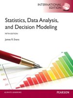
others from consuming the good, whether they have paid for it or not. Figure 5.7 shows
four possible categories into which goods can fall.
We next consider each of the four categories:
1.A private good is both rival and excludable. Food, clothing, haircuts, and many other
goods and services fall into this category. One person consuming a unit of these goods
precludes other people from consuming that unit, and no one can consume these goods

25/06/14 8:38 PM


www.downloadslide.net


Four Categories of Goods

Rival

Nonrival

Excludable

Nonexcludable

Private Goods
Examples:
Big Macs
Running shoes


Common Resources
Examples:
Tuna in the ocean
Public pasture land

Quasi-Public Goods
Examples:
Cable TV
Toll road

Public Goods
Examples:
National defense
Court system

without buying them. Although we didn’t state it explicitly, when we analyzed the demand and supply for goods and services in earlier chapters, we assumed that the goods
and services were all private goods.
2.A public good is both nonrival and nonexcludable. Public goods are often, although
not always, supplied by a government rather than private firms. The classic example
of a public good is national defense. Your consuming national defense does not interfere with your neighbor consuming it, so consumption is nonrival. You also cannot be excluded from consuming it, whether you pay for it or not. No private firm
would be willing to supply national defense because everyone can consume national
defense whether they pay for it or not. The behavior of consumers in this situation is
called free riding because individuals benefit from a good—in this case, the provision of national defense—without paying for it.
3.A quasi-public good is excludable but not rival. An example is cable television.
People who do not pay for cable television do not receive it, but one person
watching it doesn’t affect other people watching it. The same is true of a toll road.
­Anyone who doesn’t pay the toll doesn’t get on the road, but one person using the
road doesn’t interfere with someone else using the road (unless so many people
are using the road that it becomes congested). Goods that fall into this category

are called quasi-public goods.
4. A common resource is rival but not excludable. Forest land in many poor countries
is a common resource. If one person cuts down a tree, no one else can use the tree.
But if no one has a property right to the forest, no one can be excluded from using it.
As we will discuss in more detail later, people often overuse common resources.

203

MyEconLab Animation
Figure 5.7
Four Categories of Goods
Goods and services can be divided into four
categories on the basis of whether people
can be excluded from consuming them
and whether they are rival in consumption.
A good or service is rival in consumption
if one person consuming a unit of a good
means that another person cannot consume
that unit.

Public good  A good that is both
nonrival and nonexcludable.

Free riding  Benefiting from a good
without paying for it.

Common resource  A good that is
rival but not excludable.

We discussed the demand and supply for private goods in earlier chapters. For

the remainder of this chapter, we focus on the categories of public goods and common
resources. To determine the optimal quantity of a public good, we have to modify our
usual demand and supply analysis to take into account that a public good is both nonrival and nonexcludable.

The Demand for a Public Good
We can determine the market demand curve for a good or service by adding up the
quantity of the good demanded by each consumer at each price. To keep things simple,
let’s consider the case of a market with only two consumers. Figure 5.8 shows that the
market demand curve for hamburgers depends on the individual demand curves of Jill
and Joe.
At a price of $4.00, Jill demands 2 hamburgers per week and Joe demands 4. Adding horizontally, the combination of a price of $4.00 per hamburger and a quantity
demanded of 6 hamburgers will be a point on the market demand curve for hamburgers. Similarly, adding horizontally at a price of $1.50, we have a price of $1.50 and a
quantity demanded of 11 as another point on the market demand curve. A consumer’s
demand curve for a good represents the marginal benefit the consumer receives from
the good, so when we add together the consumers’ demand curves, we have not only the
market demand curve but also the marginal social benefit curve for this good, assuming
that there is no externality in consumption.

M05_HUBB9457_05_SE_C05.indd 203

25/06/14 8:38 PM


www.downloadslide.net
204

C h a p t e r 5 Externalities, Environmental Policy, and Public Goods

Price


Price

Price

$4.00

$4.00

$4.00

1.50

1.50

1.50

Jill’s
demand
0

2

3

Quantity

(a) Jill’s demand for
hamburgers

Demand =

marginal social
benefit

Joe’s
demand
0

4

8

Quantity

(b) Joe’s demand for hamburgers

6

0

11

Quantity

(c) Market demand for hamburgers

MyEconLab Animation
Figure 5.8   Constructing the Market Demand Curve for a Private Good
The market demand curve for private goods is determined by adding horizontally
the quantity of the good demanded at each price by each consumer. For instance,
in panel (a), Jill demands 2 hamburgers when the price is $4.00, and in panel (b),


Joe demands 4 hamburgers when the price is $4.00. So, a quantity of 6 hamburgers
and a price of $4.00 is a point on the market demand curve in panel (c).

How can we find the demand curve or marginal social benefit curve for a public
good? Once again, for simplicity, assume that Jill and Joe are the only consumers. Unlike
with a private good, where Jill and Joe can end up consuming different quantities, with
a public good, they will consume the same quantity. Suppose that Jill owns a service station on an isolated rural road, and Joe owns a car dealership next door. These are the
only two businesses around for miles. Both Jill and Joe are afraid that unless they hire a
security guard at night, their businesses may be burgled. Like national defense, the services of a security guard are in this case a public good: Once hired, the guard will be able
to protect both businesses, so the good is nonrival. It also will not be possible to exclude
either business from being protected, so the good is nonexcludable.
To arrive at a demand curve for a public good, we don’t add quantities at each
price, as with a private good. Instead, we add the price each consumer is willing to pay
for each quantity of the public good. This value represents the total dollar amount consumers as a group would be willing to pay for that quantity of the public good. In other
words, to find the demand curve, or marginal social benefit curve, for a private good,
we add the demand curves of individual consumers horizontally; for public goods, we
add individual demand curves vertically. Figure 5.9 shows how the marginal social
benefit curve for security guard services depends on the individual demand curves of
Jill and Joe.
The figure shows that Jill is willing to pay $8 per hour for the guard to provide
10 hours of protection per night. Joe would suffer a greater loss from a burglary, so he is
willing to pay $10 per hour for the same amount of protection. Adding the dollar amount
that each is willing to pay gives us a price of $18 per hour and a quantity of 10 hours as
a point on the marginal social benefit curve for security guard services. The figure also
shows that because Jill is willing to spend $4 per hour for 15 hours of guard services and
Joe is willing to pay $5, a price of $9 per hour and a quantity of 15 hours is another point
on the marginal social benefit curve for security guard services. MyEconLab Concept Check

The Optimal Quantity of a Public Good

We know that to achieve economic efficiency, a good or service should be produced up
to the point where the sum of consumer surplus and producer surplus is maximized, or,
alternatively, where the marginal social cost equals the marginal social benefit. Therefore, the optimal quantity of security guard services—or any other public good—will

M05_HUBB9457_05_SE_C05.indd 204

25/06/14 8:38 PM


www.downloadslide.net


Four Categories of Goods

MyEconLab Animation

Price (dollars
per hour)

Figure 5.9

$8

Constructing the Demand
Curve for a Public Good

4
Jill’s
demand
0


205

10

15

Quantity
(hours of
protection)

(a) Jill’s demand for security guard services
Price (dollars
per hour)
$10

To find the demand curve for a public good,
we add up the price at which each consumer
is willing to purchase each quantity of
the good. In panel (a), Jill is willing to pay
$8 per hour for a security guard to provide
10 hours of protection. In panel (b), Joe is
willing to pay $10 for that level of protection. Therefore, in panel (c), the price of $18
per hour and the quantity of 10 hours will
be a point on the demand curve for security
guard services.

5
Joe’s
demand

0

10

15

Quantity
(hours of
protection)

(b) Joe’s demand for security guard services
Price (dollars
per hour)
$18

9
Demand =
marginal social
benefit

0

10

15

Quantity
(hours of
protection)


(c) Total demand for security guard services

occur where the marginal social benefit curve intersects the supply curve. As with private goods, in the absence of an externality in production, the supply curve represents
the marginal social cost of supplying the good. Figure 5.10 shows that the optimal quantity of security guard services supplied is 15 hours, at a price of $9 per hour.
Will the market provide the economically efficient quantity of security guard services? One difficulty is that the individual preferences of consumers, as shown by their
demand curves, are not revealed in this market. This difficulty does not arise with
private goods because consumers must reveal their preferences in order to purchase
private goods. If the market price of Big Macs is $4.00, Joe either reveals that he is willing
to pay that much by buying it or he does without it. In our example, neither Jill nor Joe
can be excluded from consuming the services provided by a security guard once either
hires one, and, therefore, neither has an incentive to reveal her or his preferences. In this

M05_HUBB9457_05_SE_C05.indd 205

25/06/14 8:38 PM


www.downloadslide.net
206

C h a p t e r 5 Externalities, Environmental Policy, and Public Goods

MyEconLab Animation

Price
(dollars
per
hour)

Figure 5.10

The Optimal Quantity of a
Public Good
The optimal quantity of a public good is
produced where the sum of consumer surplus and producer surplus is maximized,
which occurs where the demand curve intersects the supply curve. In this case, the
optimal quantity of security guard services
is 15 hours, at a price of $9 per hour.

Supply =
marginal
social cost

$9

Demand =
marginal
social benefit
15

0

Quantity
(hours of protection)

case, though, with only two consumers, it is likely that private bargaining will result in
an efficient quantity of the public good. This outcome is not likely for a public good—
such as national defense—that is supplied by the government to millions of consumers.
Governments sometimes use cost–benefit analysis to determine what quantity of a
public good should be supplied. For example, before building a dam on a river, the federal government will attempt to weigh the costs against the benefits. The costs include
the opportunity cost of other projects the government cannot carry out if it builds the

dam. The benefits include improved flood control or new recreational opportunities
on the lake formed by the dam. However, for many public goods, including national
defense, the government does not use a formal cost–benefit analysis. Instead, the quantity of national defense supplied is determined by a political process involving Congress
and the president. Even here, of course, Congress and the president realize that tradeoffs are involved: The more resources used for national defense, the fewer resources
available for other public or private goods.
MyEconLab Concept Check

Solved Problem 5.4

MyEconLab Interactive Animation

Determining the Optimal Level of Public Goods
Suppose, once again, that Jill and Joe run businesses that are
next door to each other on an isolated road and both need

a security guard. Their demand schedules for security guard
services are as follows:

Joe

Jill

Price (dollars per hour)

Quantity (hours of protection)

Price (dollars per hour)

Quantity (hours of protection)


$20

0

$20

1

18

1

18

2

16

2

16

3

14

3

14


4

12

4

12

5

10

5

10

6

8

6

8

7

6

7


6

8

4

8

4

9

2

9

2

10

M05_HUBB9457_05_SE_C05.indd 206

25/06/14 8:38 PM


www.downloadslide.net


Four Categories of Goods


The supply schedule for security guard services is as follows:
Price (dollars per hour)

Quantity (hours of protection)

$8
10
12
14
16
18
20
22
24

1
2
3
4
5
6
7
8
9

207

a. Draw a graph that shows the optimal level of security guard services. Be sure to label the curves on
the graph.
b. Briefly explain why 8 hours of security guard protection is not an optimal quantity.


Solving the Problem
Step 1: Review the chapter material. This problem is about determining the optimal
level of public goods, so you may want to review the section “The Optimal
Quantity of a Public Good,” which begins on page 204.
Step 2: Begin by deriving the demand curve or marginal social benefit curve for security guard services. To calculate the marginal social benefit of guard services,
we need to add the prices that Jill and Joe are willing to pay at each quantity:
Demand or Marginal Social Benefit
Price (dollars per hour)

Quantity (hours of protection)

$38
34
30
26
22
18
14
10
6

1
2
3
4
5
6
7
8

9

Step 3: Answer part (a) by plotting the demand (marginal social benefit) and supply (marginal social cost) curves. The graph shows that the optimal level of
security guard services is 6 hours.
Price
(dollars
per
hour)

Supply =
marginal
social cost

$18

Demand =
marginal
social benefit
0

6

Quantity
(hours of protection)

Step 4: Answer part (b) by explaining why 8 hours of security guard protection is
not an optimal quantity. For each hour beyond 6, the supply curve is above
the demand curve. Therefore, the marginal social benefit received will be less
than the marginal social cost of supplying these hours. This results in a deadweight loss and a reduction in economic surplus.
Your Turn: For more practice, do related problem 4.4 on page 216 at the end of this chapter.


M05_HUBB9457_05_SE_C05.indd 207

MyEconLab Study Plan

25/06/14 8:38 PM


www.downloadslide.net
208

C h a p t e r 5 Externalities, Environmental Policy, and Public Goods

Common Resources
In England during the Middle Ages, each village had an area of pasture, known as the commons, on which any family in the village was allowed to graze its cows or sheep without
charge. Of course, the grass one family’s cow ate was not available for another family’s cow,
so consumption was rival. But every family in the village had the right to use the commons, so it was nonexcludable. Without some type of restraint on usage, the commons
would be overgrazed. To see why, consider the economic incentives facing a family that
was thinking of buying another cow and grazing it on the commons. The family would
gain the benefits from increased milk production, but adding another cow to the commons would create a negative externality by reducing the amount of grass available for the
cows of other families. Because this family—and the other families in the village—did not
take this negative externality into account when deciding whether to add another cow to
the commons, too many cows would be added. The grass on the commons would eventually be depleted, and no family’s cow would get enough to eat.
Tragedy of the commons  The
tendency for a common resource to
be overused.

The Tragedy of the Commons  The tendency for a common resource to be over-

used is called the tragedy of the commons. The forests in many poor countries are a

modern example. When a family chops down a tree in a public forest, it takes into account the benefits of gaining firewood or wood for building, but it does not take into
account the costs of deforestation. Haiti, for example, was once heavily forested. Today,
80 percent of the country’s forests have been cut down, primarily to be burned to create
charcoal for heating and cooking. Because the mountains no longer have tree roots to
hold the soil, heavy rains lead to devastating floods.
Figure 5.11 shows that with a common resource such as wood from a forest, the
efficient level of use, QEfficient, is determined by the intersection of the demand curve,
which represents the marginal social benefit received by consumers, and S2, which represents the marginal social cost of cutting the wood. As in our discussion of negative
externalities, the social cost is equal to the private cost of cutting the wood plus the
external cost. In this case, the external cost represents the fact that the more wood each
person cuts, the less wood there is available for others and the greater the deforestation,
which increases the chances of floods. Because each individual tree cutter ignores the
external cost, the equilibrium quantity of wood cut is QActual, which is greater than the
efficient quantity. At the actual equilibrium level of output, there is a deadweight loss, as
shown in Figure 5.11 by the yellow triangle.

Is There a Way out of the Tragedy of the Commons?  Notice that our discussion of the tragedy of the commons is very similar to our earlier discussion of negative
externalities. The source of the tragedy of the commons is the same as the source of
negative externalities: lack of clearly defined and enforced property rights. For instance,
MyEconLab Animation
Figure 5.11
Overuse of a Common
Resource
For a common resource such as wood from
a forest, the efficient level of use, QEfficient,
is determined by the intersection of the
demand curve, which represents the marginal benefit received by consumers, and S2,
which represents the marginal social cost of
cutting the wood. Because each individual
tree cutter ignores the external cost, the

equilibrium quantity of wood cut is QActual,
which is greater than the efficient quantity.
At the actual equilibrium level of output,
there is a deadweight loss, as shown by the
yellow triangle.

Benefit
or cost
(dollars
per cord)

S1 = marginal
private cost

Efficient
equilibrium

True social
cost of tree
cutting
Deadweight
loss

Cost as seen
by individual
tree cutters
Actual
equilibrium

Demand


0

M05_HUBB9457_05_SE_C05.indd 208

S2 = marginal
social cost

QEfficient

QActual

Quantity
(cords of wood)

25/06/14 8:38 PM


www.downloadslide.net


Conclusion

suppose that instead of being held as a collective resource, a piece of pastureland is
owned by one person. That person will take into account the effect of adding another
cow on the grass available to cows already using the pasture. As a result, the optimal
number of cows will be placed on the pasture. Over the years, most of the commons
lands in England were converted to private property. Most of the forestland in Haiti and
other developing countries is actually the property of the government. The failure of the
government to protect the forests against trespassers or convert them to private property is the key to their overuse.

In some situations, though, enforcing property rights is not feasible. An example is
the oceans. Because no country owns the oceans beyond its own coastal waters, the fish
and other resources of the ocean will remain a common resource. In situations in which
enforcing property rights is not feasible, two types of solutions to the tragedy of the commons are possible. If the geographic area involved is limited and the number of people
involved is small, access to the commons can be restricted through community norms and
laws. If the geographic area or the number of people involved is large, legal restrictions on
access to the commons are required. As an example of the first type of solution, the tragedy of the commons was avoided in the Middle Ages by traditional limits on the number
of animals each family was allowed to put on the common pasture. Although these traditions were not formal laws, they were usually enforced adequately by social pressure.
With the second type of solution, the government imposes restrictions on access
to the common resources. These restrictions can take several different forms, of which
taxes, quotas, and tradable permits are the most common. By setting a tax equal to the
external cost, governments can ensure that the efficient quantity of a resource is used.
Quotas, or legal limits, on the quantity of the resource that can be taken during a given
time period have been used in the United States to limit access to pools of oil that are
MyEconLab Concept Check
beneath property owned by many different persons.

209

MyEconLab Study Plan

Continued from page 185

Economics in Your Life
What’s the “Best” Level of Pollution?

At the beginning of this chapter, we asked you to think about what is the “best” level of carbon
emissions. Conceptually, this is a straightforward question to answer: The efficient level of carbon
emissions is the level for which the marginal benefit of reducing carbon emissions exactly equals the
marginal cost of reducing carbon emissions. In practice, however, this question is very difficult to answer. For example, scientists disagree about how much carbon emissions are contributing to climate

change and what the damage from climate change will be. In addition, the cost of reducing carbon
emissions depends on the method of reduction used. As a result, neither the marginal cost curve nor
the marginal benefit curve for reducing carbon emissions is known with certainty. This uncertainty
makes it difficult for policymakers to determine the economically efficient level of carbon emissions
and is the source of much of the current debate. In any case, economists agree that the total cost of
completely eliminating carbon emissions is much greater than the total benefit.

Conclusion
Government interventions in the economy, such as imposing price ceilings and price
floors, can reduce economic efficiency. But in this chapter, we have seen that the government plays an indispensable role in the economy when the absence of well-defined and
enforceable property rights keeps the market from operating efficiently. For instance,
because no one has a property right for clean air, in the absence of government intervention, firms will produce too great a quantity of products that generate air pollution.
We have also seen that public goods are nonrival and nonexcludable and are, therefore,
often supplied directly by the government.
Visit MyEconLab for a news article and analysis related to the concepts in this chapter.

M05_HUBB9457_05_SE_C05.indd 209

25/06/14 8:38 PM


www.downloadslide.net
210

C h a p t e r 5 Externalities, Environmental Policy, and Public Goods

Chapter Summary and Problems
Key Terms
Coase theorem, p. 195


Externality, p. 186

Private benefit, p. 187

Rivalry, p. 202

Command-and-control
approach, p. 200

Free riding, p. 203

Private cost, p. 186

Social benefit, p. 187

Common resource, p. 203

Market failure, p. 188

Private good, p. 202

Social cost, p. 187

Pigovian taxes and subsidies,
p. 200

Property rights, p. 188

Tragedy of the commons, p. 208


Public good, p. 203

Transactions costs, p. 194

Excludability, p. 202

5.1

Externalities and Economic Efficiency, pages 186–189
LEARNING OBJECTIVE: Identify examples of positive and negative externalities and use graphs to show how
externalities affect economic efficiency.

Summary
An externality is a benefit or cost to parties who are not involved
in a transaction. Pollution and other externalities in production
cause a difference between the private cost borne by the producer of a good or service and the social cost, which includes
any external cost, such as the cost of pollution. An externality in
consumption causes a difference between the private benefit received by the consumer and the social benefit, which includes
any external benefit. If externalities exist in production or consumption, the market will not produce the optimal level of a
good or service. This outcome is referred to as market failure.
Externalities arise when property rights do not exist or cannot
be legally enforced. Property rights are the rights individuals or
businesses have to the exclusive use of their property, including
the right to buy or sell it.

MyEconLab

Visit www.myeconlab.com to complete select
exercises online and get instant feedback.


Review Questions
1.1What is an externality? Give an example of a positive externality, and give an example of a negative externality.
1.2When will the private cost of producing a good differ from
the social cost? Give an example. When will the private
benefit from consuming a good differ from the social benefit? Give an example.
1.3How are externalities related to the efficiency of the
­competitive market equilibrium?
1.4How do market failures relate to the necessity of government intervention in certain markets?
1.5Briefly explain the relationship between property rights
and the existence of externalities.

Problems and Applications
1.6Externalities are costs and benefits that affect people who
are not directly involved in the production or consumption of a good or service. In some cases the existence of
externalities is evident; for example, when individuals

M05_HUBB9457_05_SE_C05.indd 210

use motor vehicles they consume a transportation service
and at the same time they contribute towards air pollution. However, in other cases things are not so clear. For
example, studying at a university is an activity that can
be thought to have a number of different externalities.
Would you be able to list at least two externalities that
you have observed at your university? Briefly explain your
choices.
1.7Would it be possible for an externality to be considered
positive by some people and negative by others? For example, what if Bon Jovi was performing in an open stadium
and people outside were able to hear the music?
1.8Yellowstone National Park is in bear country. The National
Park Service, at its Yellowstone Web site, states the following about camping and hiking in bear country:

Do not leave packs containing food unattended, even for a few minutes. Allowing
a bear to obtain human food even once often results in the bear becoming aggressive
about obtaining such food in the future.
Aggressive bears present a threat to human
safety and eventually must be destroyed or
removed from the park. Please obey the law
and do not allow bears or other wildlife to
obtain human food.
What negative externality does obtaining human food
pose for bears? What negative externality do bears obtaining human food pose for future campers and hikers?
Source: National Park Service, Yellowstone National Park, “Backcountry Camping and Hiking,” June 7, 2013, www.nps.gov/yell/­
planyourvisit/backcountryhiking.htm.

1.9Every year at the beginning of flu season, many people, including the elderly, get a flu shot to reduce their chances of
contracting the flu. One result is that people who do not
get a flu shot are less likely to contract the flu.
a.
What type of externality (negative or positive) arises
from getting a flu shot?
b.
On the graph that follows, show the effects of this
­e xternality by drawing in and labelling any additional curves that are needed and by labeling the

25/06/14 8:38 PM


www.downloadslide.net


Chapter Summary and Problems


efficient quantity and the efficient price of flu shots.
Label the area representing deadweight loss in this
market.
Price of
a flu shot

S = marginal
social cost

PMarket

D = marginal
private benefit
QMarket

Quantity of
flu shots

1.10John Cassidy, a writer for the New Yorker magazine,
wrote a blog post arguing against New York City’s having installed bike lanes. Cassidy complained that the bike
lanes had eliminated traffic lanes on some streets as well
as some on-street parking. A writer for the Economist
magazine disputed Cassidy’s argument with the following comment: “I hate to belabour the point, but driving,
as it turns out, is associated with a number of negative
externalities.” What externalities are associated with
driving? How do these externalities affect the debate over
whether big cities should install more bike lanes?
Sources: John Cassidy, “Battle of the Bike Lanes,” New Yorker, March 8,
2011; and “The World Is His Parking Spot,” Economist, March 9, 2011.


1.11In a study at a large state university, students were randomly assigned roommates. Researchers found that, on
average, males assigned to roommates who reported
drinking alcohol in the year before entering college had
GPAs one-quarter point lower than those assigned to nondrinking roommates. For males who drank frequently before college, being assigned to a roommate who also drank
frequently before college reduced their GPAs by two-thirds
of a point. Draw a graph showing the price of alcohol and
the quantity of alcohol consumption on college campuses.
Include in the graph the demand for drinking and the private and social costs of drinking. Label any deadweight
loss that arises in this market.
Source: Michael Kremer and Dan M. Levy, “Peer Effects and Alcohol
Use among College Students,” Journal of Economic Perspectives, Vol. 22,
No. 3, Summer 2008, pp. 189–206.

1.12Tom and Jacob are college students. Each of them will
probably get married later and have two or three children.
Each knows that if he studies more in college, he’ll get a
better job and earn more money. Earning more will enable them to spend more on their future families for things
such as orthodontia, nice clothes, admission to expensive colleges, and travel. Tom thinks about the potential

M05_HUBB9457_05_SE_C05.indd 211

211

benefits to his potential children when he decides how
much studying to do. Jacob doesn’t.
a.
What type of externality arises from studying?
b.
Draw a graph showing this externality, contrasting the

responses of Tom and Jacob. Who studies more? Who
acts more efficiently? Briefly explain.
1.13 Fracking, or hydraulic fracturing, has been used more
frequently in recent years to drill for oil and natural gas
that previously was too expensive to obtain. According
to an article in the New York Times, “horizontal drilling has enabled engineers to inject millions of gallons of
high-pressure water directly into layers of shale to create the fractures that release the gas. Chemicals added
to the water dissolve minerals, kill bacteria that might
plug up the well, and insert sand to prop open the fractures.” Experts are divided about whether fracking results in significant pollution, but some people worry
that chemicals used in fracking might lead to pollution
of underground supplies of water used by households
and farms.
a.
First, assume that fracking causes no significant pollution. Use a demand and supply graph to show the effect
of fracking on the market for natural gas.
b.
Now assume that fracking does result in pollution. On
your graph from part (a), show the effect of fracking.
Be sure to carefully label all curves and all equilibrium
points.
c.
In your graph in part (b), what has happened to the
efficient level of output and the efficient price in the
market for natural gas compared with the situation before fracking? Can you be certain that the efficient level
of output and the efficient price have risen or fallen as a
result of fracking? Briefly explain.
Source: Susan L. Brantley and Anna Meyendorff, “The Facts on
Fracking,” New York Times, March 13, 2013.

1.14 It is widely believed that football grounds generate a

number of negative externalities on their surrounding
areas. This could probably be because they are located
in high-density residential areas. Therefore, it has often
been suggested that relocating football clubs to areas
that have a low-density population or in the outskirts
of a town would help in eliminating some of those
negative externalities, if not all. Mason and Moncrieff
(1993) have discussed their doubts about this proposed
alternative being a solution for the problems related to
football grounds and having them in a neighborhood.
What types of negative externalities would having a
football field in a high-density residential area
­g enerate? Explain why having such football facilities would generate negative externalities in residential ­areas. Is hooliganism seen as the greater nuisance
as compared to traffic congestion or car parking?
­H ypothesize why relocating the football stadiums
would not solve the negative externality issue that is
faced in such situations. Also, if the space were used
for a non-football activity, a rock concert for example,
would the negative externalities be less or more?
Source: C. Mason & A. Moncrieff, 1993, “The effect of relocation on
the externality fields of football stadia: The case of St Johnstone FC,”
The Scottish Geographical Magazine 109(2), 96–105; John Bale, Handbook of Sports Studies, SAGE Publications Ltd., 2000.

25/06/14 8:38 PM


www.downloadslide.net
212

C h a p t e r 5 Externalities, Environmental Policy, and Public Goods


1.15In an article in the agriculture magazine Choices, Oregon
State University economist JunJie Wu made the following
observation about the conversion of farmland to urban
development:
Land use provides many economic and social
benefits, but often comes at a substantial cost
to the environment. Although most economic
costs are figured into land use decisions, most
environmental externalities are not. These environmental “externalities” cause a divergence
between private and social costs for some land
uses, leading to an inefficient land allocation.
For example, developers may not bear all the



5.2



environmental and infrastructural costs generated by their projects. Such “market failures”
provide a justification for private conservation efforts and public land use planning and
regulation.
What does the author mean by market failures and inefficient land allocation? Explain why the author describes inefficient land allocation as a market failure. Illustrate your
argument with a graph showing the market for land to be
used for urban development.
Source: JunJie Wu, “Land Use Changes: Economic, Social, and Environmental Impacts,” Choices, Vol. 23, No. 4, Fourth Quarter 2008,
pp. 6–10.

Private Solutions to Externalities: The Coase Theorem,

pages 189–195
LEARNING OBJECTIVE: Discuss the Coase theorem and explain how private bargaining can lead to
economic efficiency in a market with an externality.

Summary
Externalities and market failures result from incomplete property rights or from the difficulty of enforcing property rights in
certain situations. When an externality exists, and the efficient
quantity of a good is not being produced, the total cost of reducing the externality is usually less than the total benefit. According to the Coase theorem, if transactions costs are low, private
bargaining will result in an efficient solution to the problem of
externalities.

MyEconLab

Visit www.myeconlab.com to complete select
exercises online and get instant feedback.

Review Questions
2.1Is talking about an economically efficient (sometimes
­labeled “optimal”) level of pollution paradoxical? Explain.
2.2Under what conditions would private solutions to the problem of externalities be possible? Briefly describe them.
2.3What are transactions costs? When are we likely to see private solutions to the problem of externalities?

Problems and Applications
2.4Is it ever possible for an increase in pollution to make society better off? Briefly explain, using a graph like Figure 5.3
on page 191.

M05_HUBB9457_05_SE_C05.indd 212

2.5If the marginal cost of reducing a certain type of pollution is zero, should all that type of pollution be eliminated?
Briefly explain.

2.6Discuss the factors that determine the marginal cost
of reducing crime. Discuss the factors that determine
the marginal benefit of reducing crime. Would it be
economically efficient to reduce the amount of crime to
zero? Briefly explain.
2.7In discussing the reduction of air pollution in the developing world, Richard Fuller of the Blacksmith Institute, an environmental organization, observed, “It’s the 90/10 rule. To do
90 percent of the work only costs 10 percent of the money. It’s
the last 10 percent of the cleanup that costs 90 percent of the
money.” Why should it be any more costly to clean up the
last 10 percent of polluted air than to clean up the first 90
percent? What trade-offs would be involved in cleaning up
the final 10 percent?
Source: Tiffany M. Luck, “The World’s Dirtiest Cities,” Forbes,
­February 28, 2008.

2.8[Related to the Making the Connection on page 190]
In the first years following the passage of the Clean Air Act
in 1970, air pollution declined sharply, and there were important health benefits, including a decline in infant mortality. According to an article in the Economist magazine,
however, recently some policymakers “worry that the EPA
is constantly tightening restrictions on pollution, at ever
higher cost to business but with diminishing returns in
terms of public health.”
a.
Why might additional reductions in air pollution come
at “ever higher cost”? What does the article mean that

25/06/14 8:38 PM


www.downloadslide.net



Chapter Summary and Problems

these reductions will result in “ever diminishing returns in terms of public health”?
b.
How should the federal government decide whether
further reductions in air pollution are needed?
Source: “Soaring Emissions,” Economist, June 2, 2011.

2.9[Related to the Don’t Let This Happen to You on page
193] Briefly explain whether you agree or disagree
with the following statement: “Sulfur dioxide emissions
cause acid rain and breathing difficulties for people
with respiratory problems. The total benefit to society
is greatest if we completely eliminate sulfur dioxide
emissions. Therefore, the economically efficient level of
emissions is zero.”

5.3

213

2.10 Think about the Coase theorem. Assume that a polluting
plant is only damaging one farmer, who has fields all
around the plant. There are no transaction costs; both
the plant owner and the farmer have perfect knowledge about the negative externality that is being caused
by the plant. Can the plant owner buy the “right to
pollute”?
2.11 [Related to the Making the Connection on page 193]

We know that owners of apple orchards and beehives are
able to negotiate private agreements. Is it likely that as a
result of these private agreements, the market supplies the
efficient quantities of apple trees and beehives? Are there
any real-world difficulties that might stand in the way of
achieving this efficient outcome?

Government Policies to Deal with Externalities, pages 195–202
LEARNING OBJECTIVE: Analyze government policies to achieve economic efficiency in a market with
an externality.

Summary

Problems and Applications

When private solutions to externalities are unworkable, the
government sometimes intervenes. One way to deal with a
negative externality in production is to impose a tax equal to
the cost of the externality. The tax causes the producer of the
good to internalize the externality. The government can deal
with a positive externality in consumption by giving consumers a subsidy, or payment, equal to the value of the externality. Government taxes and subsidies intended to bring about
an efficient level of output in the presence of externalities are
called Pigovian taxes and subsidies. Although the federal government has sometimes used subsidies and taxes to deal with
externalities, in dealing with pollution it has more often used
a command-and-control approach. A command-and-control
approach involves the government imposing quantitative
­limits on the amount of pollution allowed or requiring firms to
install specific pollution control devices. Direct pollution controls of this type are not economically efficient, however. As a
result, economists generally prefer reducing pollution by using
market-based policies.


3.4The author of a newspaper article remarks that many
economists “support Pigovian taxes because, in some
sense, we are already paying them.” In what sense might
consumers in a market be “paying” a Pigovian tax even if
the government hasn’t imposed an explicit tax?

MyEconLab

Visit www.myeconlab.com to complete select
exercises online and get instant feedback.

Review Questions
3.1Define a Pigovian tax. Briefly list and explain the problems
related to the implementation of the tax.
3.2What does it mean for a producer or consumer to internalize an externality? What would cause a producer or
consumer to internalize an externality?
3.3Why do most economists prefer tradable emission allowances to the command-and-control approach to
pollution?

M05_HUBB9457_05_SE_C05.indd 213

Source: Adam Davidson, “Should We Tax People for Being Annoying?” New York Times, January 8, 2013.

3.5The British government has recently started to consider
the introduction of a 20 percent tax on sugary drinks. Why
has this been positively received by the National Health
Service?
Source: “Sugary drinks tax ‘effective public health measure’, ” BBC
News health, November 1, 2013.


3.6Many antibiotics that once were effective in eliminating
infections no longer are because bacteria have evolved to
become resistant to them. Some bacteria are now resistant
to all but one or two existing antibiotics. Some policymakers have argued that pharmaceutical companies should
receive subsidies for developing new antibiotics. A newspaper article states:
While the notion of directly subsidizing drug
companies may be politically unpopular in
many quarters, proponents say it is necessary
to bridge the gap between the high value that
new antibiotics have for society and the low
returns they provide to drug companies.
Is there a positive externality in the production of antibiotics? Should firms producing every good where there is a
gap between the value of the good to society and the profit
to the firms making the good receive subsidies? Briefly
explain.
Source: Andrew Pollack, “Antibiotics Research Subsidies Weighed by
U.S.,” New York Times, November 5, 2010.

25/06/14 8:38 PM


www.downloadslide.net
214

C h a p t e r 5 Externalities, Environmental Policy, and Public Goods

3.7A newspaper article has the headline: “Should We Tax
People for Being Annoying?”
a.

Do annoying people cause a negative externality?
Should they be taxed? Do crying babies on a bus or
plane cause a negative externality? Should the babies
(or their parents) be taxed?
b.
Do people who plant flowers and otherwise have beautiful gardens visible from the street cause a positive
externality? Should these people receive a government
subsidy?
c.
Should every negative externality be taxed? Should
every positive externality be subsidized? How might
the government decide whether using Pigovian taxes
and subsidies is appropriate?

a.
Explain how a government can use a tax on dry cleaning to bring about the efficient level of production.
What should the value of the tax be?
b.
How large is the deadweight loss (in dollars) from
excessive dry cleaning, according to the figure?
3.11 [Related to Solved Problem 5.3 on page 198] Companies that produce toilet paper bleach the paper to make
it white. Some paper plants discharge the bleach into rivers and lakes, causing substantial environmental damage.
Suppose the following graph illustrates the situation in the
toilet paper market.

Price
(per ton
of toilet
Source: Adam Davidson, “Should We Tax People for Being Annoy- paper)


S2 = marginal social cost
S1 = marginal
private cost

ing?” New York Times, January 8, 2013.

3.8Is government intervention (for instance in the form of
subsidies) always justified in the case of positive externalities? Is the fact that all activities create benefits that
may not be appropriable by their creators a debatable
statement? Briefly discuss the reasons for your answer.
3.9[Related to Solved Problem 5.3 on page 198] Solved
Problem 5.3 contains the statement: “Of course, the government actually collects the tax from sellers rather than
from consumers, but we get the same result whether the
government imposes a tax on the buyers of a good or on
the sellers.” Demonstrate that this statement is correct by
solving the problem assuming that the increase in the tax
on gasoline shifts the supply curve rather than the demand
curve.
3.10 [Related to Solved Problem 5.3 on page 198] The fumes
from dry cleaners can contribute to air pollution. Suppose the following graph illustrates the situation in the dry
cleaning market.
Price
(dollars
per item
cleaned)

S2 = marginal
social cost
S1 = marginal
private cost


$7.50
7.25
7.15

D

0

M05_HUBB9457_05_SE_C05.indd 214

600,000 750,000
Quantity
(items cleaned per week)

$150
125
100

Demand

0

350,000 450,000

Quantity
(tons of toilet paper
produced per week)

Explain how the federal government can use a tax on toilet paper to bring about the efficient level of production.

What should be the value of the tax?

3.12 [Related to the Making the Connection on page 196]
Eric Finklestein, an economist at Duke University, has argued that the external costs from being obese are larger
than the external costs from smoking because “the mortality effect for obesity is much smaller than it is for smoking
and the costs start much earlier in life.”
a.
What does Finklestein mean by the “mortality effect”? Why would the mortality effect of obesity being
smaller than the mortality effect of smoking result in
obesity having a larger external cost?
b.
Tobacco taxes have been more politically popular than
taxes on soda. Why might the general public be more
willing to support cigarette taxes than soda taxes?
Source: David Leonhardt, “Obama Likes Some Sin Taxes More Than
Others,” New York Times, April 10, 2013.

3.13A few years ago, Governor Deval Patrick of Massachusetts
proposed that criminals would have to pay a “safety fee” to
the government. The size of the fee would be based on the
seriousness of the crime (that is, the fee would be larger for
more serious crimes).

25/06/14 8:38 PM


www.downloadslide.net


Chapter Summary and Problems


a.
Is there an economically efficient amount of crime?
Briefly explain.
b.
Briefly explain whether the “safety fee” is a Pigovian tax
of the type discussed in this chapter.
Source: Michael Levenson, “Patrick Proposes New Fee on Criminals,”
Boston Globe, January 14, 2007.

3.14The following graph illustrates the situation in the dry
cleaning market assuming that the marginal social cost
of the pollution increases as the quantity of items cleaned
per week increases. The graph includes two demand
curves: one for a smaller city, DS, and the other for a
larger city, DL.
Price
(dollars
per item
cleaned)
$6.60

S1 = marginal
private cost

5.60
DL

5.40


a.
Explain why the marginal social cost curve has a different slope than the marginal private cost curve.
b.
What tax per item cleaned will achieve economic
efficiency in the smaller city? In the larger city?
Explain why the efficient tax is different in the two
cities.
3.15 [Related to the Chapter Opener on page 185] According to an article in the New York Times: “Top economists
agree a tax on fuels and the carbon they spew into the atmosphere would be the cheapest way to combat climate
change.” Why would a carbon tax be a cheaper way to reduce carbon dioxide emissions than the command-andcontrol approach of ordering utilities to emit less carbon
dioxide and automobile companies to produce more fuelefficient cars?
Source: Eduardo Porter, “In Energy Taxes, Tools to Help Tackle Climate Change,” New York Times, January 29, 2013.

S2 = marginal
social cost

5.85

215

5.25

3.16 [Related to the Making the Connection on page 201]
Think about the economically efficient level of pollution
reduction, which has been mentioned in this Chapter in
relation to the global warming problem.
a.
Is it possible for us to fully understand the costs that
are related to global warming?
b.

Why does the fact that the world governments are willing to start taking serious and concrete measures to
tackle the problem of global warming, within the next
few years, seem unrealistic?

5.00
DS

Quantity
(items cleaned per week)

0

5.4

Four Categories of Goods, pages 202–209
LEARNING OBJECTIVE: Explain how goods can be categorized on the basis of whether they are rival or
excludable and use graphs to illustrate the efficient quantities of public goods and common resources.

Summary
There are four categories of goods: private goods, public goods,
quasi-public goods, and common resources. Private goods are
both rival and excludable. Rivalry means that when one person
consumes a unit of a good, no one else can consume that unit.
Excludability means that anyone who does not pay for a good
cannot consume it. Public goods are both nonrival and nonexcludable. Private firms are usually not willing to supply public
goods because of free riding. Free riding involves benefiting from
a good without paying for it. Quasi-public goods are excludable
but not rival. Common resources are rival but not excludable.
The tragedy of the commons refers to the tendency for a common resource to be overused. The tragedy of the commons results
from a lack of clearly defined and enforced property rights. We

find the market demand curve for a private good by adding the

M05_HUBB9457_05_SE_C05.indd 215

quantity of the good demanded by each consumer at each price.
We find the demand curve for a public good by adding vertically
the price each consumer would be willing to pay for each quantity
of the good. The optimal quantity of a public good occurs where
the demand curve intersects the curve representing the marginal
cost of supplying the good.

MyEconLab

Visit www.myeconlab.com to complete select
exercises online and get instant feedback.

Review Questions
4.1Define the four categories of goods illustrated in the chapter. How would you distinguish one from another?

25/06/14 8:38 PM


www.downloadslide.net
216

C h a p t e r 5 Externalities, Environmental Policy, and Public Goods

4.2What is free riding? How is free riding related to the
­tendency of a public good to create market failure?
4.3What is the tragedy of the commons? How can it be

avoided?

Problems and Applications
4.4[Related to Solved Problem 5.4 on page 206] Suppose
that Jill and Joe are the only two people in the small town
of Andover. Andover has land available to build a park of
no more than 9 acres. Jill and Joe’s demand schedules for
the park are as follows:
Joe
Price per Acre

Number of Acres

$10

0

9

1

8

2

7

3

6


4

5

5

4

6

3

7

2

8

1

9

Jill
Price per Acre

Number of Acres

$15


0

14

1

13

2

12

3

11

4

10

5

9

6

8

7


7

8

6

9

The supply curve is as follows:
Price per Acre

Number of Acres

$11

1

13

2

15

3

17

4

19


5

21

6

23

7

25

8

27

9

M05_HUBB9457_05_SE_C05.indd 216

a.
Draw a graph showing the optimal size of the park. Be
sure to label the curves on the graph.
b.
Briefly explain why a park of 2 acres is not optimal.
4.5Commercial whaling has been described as a modern
example of the tragedy of the commons. Briefly explain
whether you agree.
4.6Three researchers have recently proposed (Costello et al.

2012) to put a price on killing whales. This would in turn
allow conservationists and whalers alike to bid on the right
to take them. Do you think that this proposal should be
taken seriously?
Source: C. Costello, S. Gaines, and L.R. Gerber, 2012, “Conservation
science: A market approach to saving the whales,” Nature 481.7380,
139–140.

4.7The more frequently bacteria are exposed to antibiotics,
the more quickly the bacteria will develop resistance to the
antibiotics. An article from MayoClinic.com includes the
following about antibiotic use:
If antibiotics are used too often for things
they can’t treat—like colds, flu or other viral
infections—not only are they of no benefit, they
become less effective against the bacteria they’re
intended to treat…. Nearly all significant bacterial infections in the world are becoming
resistant to commonly used antibiotics. When
you misuse antibiotics, you help create resistant microorganisms that can cause new and
hard-to-treat infections.
Briefly discuss in what sense antibiotics can be considered
a common resource.
Source: Mayo Clinic Staff, “Antibiotics: Misuse Puts You and Others
at Risk,” www.MayoClinic.com, February 4, 2012.

4.8Put each of these goods or services into one of the boxes
in Figure 5.7 on page 203. That is, categorize them as private goods, public goods, quasi-public goods, or common
resources.
a.
A television broadcast of baseball’s World Series

b.
Home mail delivery
c.
Education in a public school
d.
Education in a private school
e.
Hiking in a park surrounded by a fence
f.
Hiking in a park not surrounded by a fence
g.
An apple
4.9How do private goods differ from public goods with regard to the construction of their respective market demand curves? Discuss with appropriate examples.
4.10Do you think it possible to consider public transportation
services to be public goods? Briefly explain why free riding
is frequently mentioned as one of the problems affecting
public transport services in an economy?

25/06/14 8:38 PM


www.downloadslide.net


4.11In the early 1800s, more than 60 million American
bison (commonly known as the buffalo) roamed the Great
Plains. By the late 1800s, the buffalo was nearly extinct.
Considering the four categories of goods discussed in this
chapter, why might it be that hunters nearly killed buffalo
to extinction but not cattle?

4.12William Easterly in The White Man’s Burden shares the following account by New York University Professor L
­ eonard
Wantchekon of how Professor Wantchekon’s village in
­B enin, Africa, managed the local fishing pond when he
was growing up:
To open the fishing season, elders performed ritual tests at Amlé, a lake fifteen kilometers from
the village. If the fish were large enough, fishing

M05_HUBB9457_05_SE_C05.indd 217

Chapter Summary and Problems

217

was allowed for two or three days. If they were
too small, all fishing was forbidden, and anyone who secretly fished the lake at this time was
outcast, excluded from the formal and informal
groups that formed the village’s social structure.
Those who committed this breach of trust were
often shunned by the whole community; no one
would speak to the offender, or even acknowledge his existence for a year or more.
What economic problem were the village elders trying to
prevent? Do you think their solution was effective?
Source: William Easterly, The White Man’s Burden: Why the West’s
­Efforts to Aid the Rest Have Done So Much Ill and So Little Good, New
York: Penguin Books, 2006, p. 94.

25/06/14 8:38 PM



www.downloadslide.net

Chapter

6

Elasticity:
The Responsiveness
of Demand and Supply

Chapter Outline
and Learning
Objectives
6.1

The Price Elasticity of Demand and
Its Measurement, page 220
Define price elasticity of
demand and understand how
to measure it.

6.2

The Determinants of the Price
Elasticity of Demand, page 226
Understand the determinants
of the price elasticity of
demand.

6.3


The Relationship between Price
Elasticity of Demand and Total
Revenue, page 229
Understand the relationship
between the price elasticity of
demand and total revenue.

6.4

Other Demand Elasticities,
page 233
Define cross-price elasticity of
demand and income elasticity
of demand and understand
their determinants and how
they are measured.

6.5

Using Elasticity to Analyze the
Disappearing Family Farm,
page 235
Use price elasticity and income
elasticity to analyze economic
issues.

6.6

The Price Elasticity of Supply and

Its Measurement, page 237
Define price elasticity of supply
and understand its main
determinants and how it is
measured.

M06_HUBB9457_05_SE_C06.indd 218

25/06/14 8:49 PM


www.downloadslide.net

Do People Respond to Changes
in the Price of Gasoline?
“Get ready for a roller coaster.” This advice
came from Steve Mosby, a partner with
Admo Energy, a supplier of gasoline to retailers. Mr. Mosby was referring to swings in
gasoline prices that were predicted for the
summer of 2013. The fluctuations in gasoline prices over the previous few years had
been much larger than normal.
But do fluctuations in gas prices have
much effect on sales of gasoline? Some people would say that they don’t. These people
argue that consumers don’t vary the quantity
of gas they buy as the price fluctuates because the number of miles they need to drive
to get to work or school or to run errands
is roughly constant. Actual consumer behavior contradicts this argument. For example,
in September 2012, when the average price
of gasoline was $3.91 per gallon, U.S. consumers bought about 5 percent less gasoline
than they had during September 2011, when

the average price of gasoline was $3.66 per
gallon.
When gasoline prices have reached
$4 per gallon on several occasions in recent years, consumers found many ways to
cut back on the quantity they purchased. As
Dennis Jacobe, chief economist of Gallup,

a public opinion poll firm, put it: “At $4 a
gallon, you get people who might have
money to spend, but with the amount gasoline costs, they start to cut back in response
to the price. At $4 a gallon … they make
fewer trips.” In California, rising gas prices
have resulted in a decline in the number of
cars crossing the Golden Gate Bridge, as
commuters switch to using buses and ferries. Car dealers report that sales of smaller,
more fuel-efficient cars are increasing compared with sales of SUVs and other less fuelefficient vehicles.
All businesses have a strong interest in
knowing how much their sales will decrease
as prices rise. Governments are also interested in knowing how consumers will react
if the price of a product such as gasoline rises
following a tax increase. In this chapter, we
will explore what determines the responsiveness of the quantity demanded and the quantity supplied to changes in the market price.
Sources: Steve Everly, “‘Get Ready for a Roller Coaster’ as
Gas Prices Swing Wildly,” Kansas City Star, April 21, 2013;
Meg Handley, “Memorial Day 2013: Higher Gas Prices,
Fewer Travelers,” U.S. News & World Report, May 23, 2013;
and data on gasoline prices and consumption from the U.S.
Energy Information Administration.

Economics in Your Life

How Much Do Gas Prices Matter to You?

What factors would make you more or less responsive to price when purchasing gasoline? Have you
responded differently to price changes during different periods of your life? Why do consumers
seem to respond more to changes in gas prices at a particular service station but seem less sensitive
when gas prices rise or fall at all service stations? As you read this chapter, try to answer these questions. You can check your answers against those we provide on page 242 at the end of this chapter.

219

M06_HUBB9457_05_SE_C06.indd 219

25/06/14 8:49 PM


www.downloadslide.net
220

C h a p t er 6 Elasticity: The Responsiveness of Demand and Supply

Elasticity  A measure of how much
one economic variable responds to
changes in another economic variable.

6.1 Learning Objective
Define price elasticity of
demand and understand how
to measure it.
Price elasticity of demand  The
responsiveness of the quantity
demanded to a change in price,

measured by dividing the percentage
change in the quantity demanded of a
product by the percentage change in
the product’s price.

W

hether you are managing a service station, a pizza parlor, or a coffee shop,
you need to know how an increase or a decrease in the price of your products will affect the quantity consumers are willing to buy. We know that
cutting the price of a good increases the quantity demanded and that raising the price reduces the quantity demanded. But the critical question is: How much will the
quantity demanded change as a result of a price increase or decrease? Economists use the concept of elasticity to measure how one economic variable—such as the quantity demanded—
responds to changes in another economic variable—such as the price. For example, the
responsiveness of the quantity demanded of a good to changes in its price is called the price
elasticity of demand. Knowing the price elasticity of demand allows you to compute the effect of a price change on the quantity demanded.
We also know that the quantity of a good that consumers demand depends not just on
the price of the good but also on consumer income and on the prices of related goods. As a
manager, you would also be interested in measuring the responsiveness of demand to these
other factors. As we will see, we can use the concept of elasticity here as well. We are also
interested in the responsiveness of the quantity supplied of a good to changes in its price,
which is called the price elasticity of supply.
Elasticity is an important concept not just for business managers but for policymakers as well. If the government wants to discourage teenage smoking, it can raise the price
of cigarettes by increasing the tax on them. If we know the price elasticity of demand for
cigarettes, we can calculate how many fewer packs of cigarettes will be demanded at a higher
price. In this chapter, we will also see how policymakers use the concept of elasticity.

The Price Elasticity of Demand and Its Measurement
We know from the law of demand that when the price of a product falls, the quantity
demanded of the product increases. But the law of demand tells firms only that the
demand curves for their products slope downward. More useful is a measure of the
responsiveness of the quantity demanded to a change in price. This measure is called

the price elasticity of demand.

Measuring the Price Elasticity of Demand
We might measure the price elasticity of demand by using the slope of the demand
curve because the slope of the demand curve tells us how much quantity changes as
price changes. Using the slope of the demand curve to measure price elasticity has a
drawback, however: The measurement of slope is sensitive to the units chosen for quantity and price. For example, suppose a $1 per gallon decrease in the price of gasoline
leads to an increase in the quantity demanded from 10.1 million gallons to 10.2 million
gallons per day. The change in quantity is 0.1 million gallons, and the change in price is
-$1, so the slope is 0.1/-1 = -0.1. But if we measure price in cents, rather than in dollars, the slope is 0.1/-100 = -0.001. If we measure price in dollars and gallons in thousands, instead of millions, the slope is 100/-1 = -100. Clearly, the value we compute for
the slope can change dramatically, depending on the units we use for quantity and price.
To avoid this confusion over units, economists use percentage changes when measuring the price elasticity of demand. Percentage changes are not dependent on units
of measurement. (For a review of calculating percentage changes, see the appendix to
Chapter 1.) No matter what units we use to measure the quantity of gasoline, 10 percent
more gasoline is 10 percent more gasoline. Therefore, the price elasticity of demand is
measured by dividing the percentage change in the quantity demanded by the percentage change in the product’s price. Or:
Price elasticity of demand =

M06_HUBB9457_05_SE_C06.indd 220

Percentage change in quantity demanded
.
Percentage change in price

25/06/14 8:49 PM


www.downloadslide.net



The Price Elasticity of Demand and Its Measurement

221

It’s important to remember that the price elasticity of demand is not the same as the slope
of the demand curve.
If we calculate the price elasticity of demand for a price cut, the percentage change
in price will be negative, and the percentage change in quantity demanded will be positive. Similarly, if we calculate the price elasticity of demand for a price increase, the
percentage change in price will be positive, and the percentage change in quantity demanded will be negative. Therefore, the price elasticity of demand is always negative.
In comparing elasticities, though, we are usually interested in their relative size. So, we
often drop the minus sign and compare their absolute values. For example, although -3
is actually a smaller number than -2, we say that a price elasticity of -3 is larger than a
price elasticity of -2.
MyEconLab Concept Check

Elastic Demand and Inelastic Demand
If the quantity demanded is very responsive to changes in price, the percentage change
in quantity demanded will be greater than the percentage change in price, and the price
elasticity of demand will be greater than 1 in absolute value. In this case, demand is
elastic. For example, if a 10 percent decrease in the price of bagels results in a 20 percent
increase in the quantity of bagels demanded, then:
Price elasticity of demand =

20%
= - 2,
- 10%

and we can conclude that the demand for bagels is elastic.
When the quantity demanded is not very responsive to price, however, the percentage change in quantity demanded will be less than the percentage change in price, and
the price elasticity of demand will be less than 1 in absolute value. In this case, demand

is inelastic. For example, if a 10 percent decrease in the price of wheat results in a 5 percent increase in the quantity of wheat demanded, then:
Price elasticity of demand =

5%
= - 0.5,
- 10%

and we can conclude that the demand for wheat is inelastic.
In the special case where the percentage change in quantity demanded is equal to
the percentage change in price, the price elasticity of demand equals -1 (or 1 in absolute
value). In this case, demand is unit elastic.
MyEconLab Concept Check

An Example of Computing Price Elasticities
Suppose you own a service station, and you are trying to decide whether to cut the price
you are charging for a gallon of gas. You are currently at point A in Figure 6.1, selling
1,000 gallons per day at a price of $4.00 per gallon. How many more gallons you will sell
by cutting the price to $3.70 depends on the price elasticity of demand for gasoline at
your service station. Let’s consider two possibilities: If D1 is the demand curve for gasoline at your station, your sales will increase to 1,200 gallons per day, point B. But if D2 is
your demand curve, your sales will increase only to 1,050 gallons per day, point C. We
might expect—correctly, as we will see—that between these points, demand curve D1 is
elastic, and demand curve D2 is inelastic.
To confirm that D1 is elastic between these points and that D2 is inelastic, we need
to calculate the price elasticity of demand for each curve. In calculating price elasticity between two points on a demand curve, though, we face a problem because we get
a different value for price increases than for price decreases. Suppose we calculate the
price elasticity for D1 as the price is cut from $4.00 to $3.70. This 7.5 percent price cut
increases the quantity demanded from 1,000 gallons to 1,200 gallons, or by 20 percent.
Therefore, the price elasticity of demand between points A and B is 20/-7.5 = -2.7. Now
let’s calculate the price elasticity for D1 as the price is increased from $3.70 to $4.00. This
8.1 percent price increase causes a decrease in the quantity demanded from 1,200 gallons

to 1,000 gallons, or by 16.7 percent. So, now our measure of the price elasticity of demand between points A and B is -16.7/8.1 = -2.1. It can be confusing to have different

M06_HUBB9457_05_SE_C06.indd 221

Elastic demand  Demand is elastic
when the percentage change in the
quantity demanded is greater than
the percentage change in price, so
the price elasticity is greater than 1 in
absolute value.

Inelastic demand  Demand is
inelastic when the percentage change
in quantity demanded is less than
the percentage change in price, so
the price elasticity is less than 1 in
absolute value.

Unit-elastic demand  Demand is unit
elastic when the percentage change
in quantity demanded is equal to the
percentage change in price, so the
price elasticity is equal to 1 in absolute
value.

25/06/14 8:49 PM


www.downloadslide.net
222


C h a p t er 6 Elasticity: The Responsiveness of Demand and Supply

MyEconLab Animation
Figure 6.1
Elastic and Inelastic Demand
Along D 1 , cutting the price from $4.00
to $3.70 increases the number of gallons
­d emanded from 1,000 to 1,200 per day.
Because the percentage change in quantity
demanded is greater than the percentage
change in price (in absolute value), d­ emand
is elastic between point A and point B.
Along D 2 , cutting the price from $4.00
to $3.70 increases the number of gallons
­demanded only from 1,000 to 1,050 per day.
Because the percentage change in quantity
demanded is smaller than the percentage
change in price (in absolute value), demand
is inelastic between point A and point C.

Price
(dollars
per
gallon)
D2 is inelastic
between point
A and point C.

$4.00


A
C

3.70

B

D1 is elastic
between point
A and point B.
D1

D2

0

1,000 1,050

1,200

Quantity
(gallons per day)

values for the price elasticity of demand between the same two points on the same demand curve. As we will see in the next section, economists use a formula that allows
them to avoid this confusion when calculating elasticities.
MyEconLab Concept Check

The Midpoint Formula
We can use the midpoint formula to ensure that we have only one value of the price

elasticity of demand between the same two points on a demand curve. The midpoint
formula uses the average of the initial and final quantities and the initial and final prices.
If Q1 and P1 are the initial quantity and price, and Q2 and P2 are the final quantity and
price, the midpoint formula is:
Price elasticity of demand =

1Q2 - Q12
1P2 - P12
,
.
Q1 + Q2
P1 + P2
b
b
a
a
2
2

The midpoint formula may seem challenging at first, but the numerator is just the
change in quantity divided by the average of the initial and final quantities, and the
denominator is just the change in price divided by the average of the initial and final
prices.
Let’s apply the formula to calculating the price elasticity of D1 in Figure 6.1. Between
point A and point B on D1, the change in quantity is 200, and the average of the two
quantities is 1,100. Therefore, there is an 18.2 percent change in quantity demanded.
The change in price is -$0.30, and the average of the two prices is $3.85. Therefore,
there is a -7.8 percent change in price. So, the price elasticity of demand is 18.2/-7.8 =
-2.3. Notice these three results from calculating the price elasticity of demand using the
midpoint formula:

1.As we suspected from examining Figure 6.1, demand curve D1 is elastic between
points A and B.
2.The value for the price elasticity calculated using the midpoint formula is between
the two values we calculated earlier.
3.The midpoint formula will give us the same value whether we are moving from the
higher price to the lower price or from the lower price to the higher price.
We can also use the midpoint formula to calculate the elasticity of demand between point A
and point C on D2. In this case, there is a 4.9 percent change in quantity and a -7.8 percent
change in price. So, the elasticity of demand is 4.9/-7.8 = -0.6. Once again, as we suspected,
demand curve D2 is price inelastic between points A and C.
MyEconLab Concept Check

M06_HUBB9457_05_SE_C06.indd 222

25/06/14 8:49 PM


www.downloadslide.net


The Price Elasticity of Demand and Its Measurement

Solved Problem 6.1

223

MyEconLab Interactive Animation

Calculating the Price Elasticity of Demand
Suppose you own a service station, and you are currently

selling gasoline for $3.50 per gallon. At this price, you can
sell 2,000 gallons per day. You are considering cutting the
price to $3.30 to attract drivers who have been buying their
gas at competing stations. The following graph shows two
possible increases in the quantity of gasoline sold as a result

of your price cut. Use the information in the graph to calculate the price elasticity between these two prices on each
of the demand curves. Use the midpoint formula in your
calculations. State whether each demand curve is elastic or
inelastic between these two prices.

Price
(dollars
per
gallon)

A

$3.50

B

C

3.30

D1

D2


2,000 2,100

0

2,500

Quantity
(gallons per day)

Solving the Problem
Step 1: Review the chapter material. This problem requires calculating the price
elasticity of demand, so you may want to review the material in the section
“The Midpoint Formula,” which begins on page 222.
Step 2: To begin using the midpoint formula, calculate the average quantity and
the average price for demand curve D1.
Average quantity =

2,000 + 2,500
= 2,250
2

Average price =

+3.50 + +3.30
= +3.40
2

Step 3: Now calculate the percentage change in the quantity demanded and the
percentage change in price for demand curve D1.
Percentage change in quantity demanded =

Percentage change in price =

M06_HUBB9457_05_SE_C06.indd 223

2,500 - 2,000
* 100 = 22.2%
2,250
+3.30 - +3.50
* 100 = - 5.9%
+3.40

25/06/14 8:49 PM