Solution manual investments 10th by jones ch07
Bạn đang xem bản rút gọn của tài liệu. Xem và tải ngay bản đầy đủ của tài liệu tại đây (63.98 KB, 16 trang )
Chapter 7:
Expected Return and Risk
CHAPTER OVERVIEW
Part II provides a concise, but complete, coverage of
returns and risk—all that a student in a beginning Investments
course needs. Chapter 7 concludes Part II with a discussion of
expected return and risk, whereas Chapter 6 focuses exclusively
on realized return and risk. This organization allows the reader
to focus on expected return and risk in Chapter 7 where portfolio
theory, which is based on expected returns, is developed.
Chapter 7 covers basic portfolio theory, allowing students
to be exposed to the most important, basic concepts of
diversification, Markowitz portfolio theory, and capital market
theory relatively early in the semester. They can then use these
concepts throughout the remaining chapters. For example, it is
very useful to know the implications of saying that stock A is
very highly correlated with stock C, or with the market, and to
be able to use the CAPM in some basic applications.
Chapter 7 serves as an introduction to portfolio theory. It
is a standard treatment of basic portfolio theory, centering on
the important building blocks of the Markowitz model. Students
learn about such well known concepts as diversification,
efficient portfolios, the risk of the portfolio, covariances, and
so forth.
The first part of the chapter discusses the estimation of
individual security return and risk, which provides the basis for
considering portfolio return and risk in the next section. It
begins with a discussion of uncertainty, and develops the concept
of a probability distribution. The important calculation of
expected value, or, as used here, expected return, is presented,
as is the equation for standard deviation.
The next part of the chapter presents the Markowitz model
along the standard dimensions of efficient portfolios, the inputs
needed, and so forth. The discussion first examines expected
portfolio return and risk. The portfolio risk discussion shows
why portfolio risk is not a weighted average of individual
security risks, which leads naturally into a discussion of
analyzing portfolio risk. The concept of risk reduction is
84
illustrated for the cases of independent returns (the insurance
principle), random diversification, and Markowitz
diversification.
Correlation coefficients and covariances are explained in
detail. This is a very standard discussion.
The calculation of portfolio risk is explained in two
stages, starting with the two-security case and progressing to
the n-security case. Sufficient detail is provided in order for
students to really understand the concept of calculating
portfolio risk using the Markowitz model, and why the problem of
the large number of covariances is significant.
Efficient portfolios are explained and illustrated in brief
fashion so that this concept can be referred to throughout the
course. This concept is elaborated on further in Chapter 19.
Because of its importance, the concepts of diversifiable and
non-diversifiable risk are explained in Chapter 7. This allows
instructors to discuss systematic risk throughout the course, and
the related concept of beta, which is discussed next.
Chapter 7 concludes with a brief discussion of the CAPM, and
the concept of beta. This allows students to use the concept
when necessary to calculate a required rate of return, or for
other purposes. The final issue mentioned is that of the SML.
This discussion gives students what they need to use the CAPM in
the course without getting bogged down in great detail with
Capital Market Theory, which is discussed in detail in Chapter
20.
CHAPTER OBJECTIVES
To explain the meaning and calculation of expected return
and risk for individual securities using probabilities.
To fully explain the concepts of expected return and risk
for portfolios, based on correlations/covariances.
To present the basics of Markowitz portfolio theory,
including the concept of efficient portfolios.
85
To develop and analyze the basics of systematic risk, beta,
the CAPM and the SML, for use throughout the course.
86
MAJOR CHAPTER HEADINGS [Contents]
Dealing With Uncertainty
Using Probability Distributions
Calculating Expected Return
[expected value/expected return]
Calculating Risk
[standard deviation using probabilities]
Portfolio Return And Risk
Portfolio Expected Return
[portfolio weights; portfolio expected return is a weighted
average of individual security returns]
Portfolio Risk
[portfolio risk is not a weighted average]
Analyzing Portfolio Risk
Risk Reduction: The Insurance Principle
[insurance principle—risk sources are independent]
Diversification
[random diversification; international diversification; how
many securities are needed to diversify properly?]
Markowitz Diversification
[basic ideas of Markowitz]
Measuring Comovements In Security Returns
Markowitz Portfolio Theory
[description; the basic concepts]
The Correlation Coefficient
[description; graphs of perfect positive correlation,
perfect negative correlation, 0.55 positive correlation]
Covariance
[description; relation with correlation coefficient]
87
Calculating Portfolio Risk
The Two-Security Case
[detailed example and explanation]
The n-Security Case
[formula; explanation; the variance-covariance matrix
illustrated]
Simplifying the Markowtiz Analysis
[the problem with too many covariances]
Efficient Portfolios
[the attainable set and the efficient set of portfolios]
Diversifiable Risk Versus Nondiversifiable Risk
[the concepts of systematic and nonsystematic risk—what
diversification can accomplish]
The Capital Asset Pricing Model
[the concept of beta; graphs of beta]
The CAPM’s Expected Reeturn-Beta Relationship
[the CAPM model; the SML]
POINTS TO NOTE ABOUT CHAPTER 7
Tables and Figures
NOTE: The figures and tables in this chapter are either the
standard figures typically seen in portfolio theory or
illustrate calculations and examples. As such, they can be
referred to directly or instructors can substitute their own
figures and examples without any loss of continuity.
88
Table 7-1 illustrates the calculation of standard deviation
when probabilities are involved.
Table 7-2 shows the expected standard deviation of annual
portfolio returns for various numbers of stocks in a portfolio.
Table 7-3 illustrates the variance-covariance matrix
involved in calculating the standard deviation of a portfolio of
two securities and of four securities. The point illustrated is
that the number of covariances involved increases quickly as more
securities are considered.
Figure 7-1 illustrates a discrete and a continuous
probability distribution.
Figure 7-2 illustrates the concept of risk reduction when
returns are independent. Risk continues to decline as the number
of observations increase.
Figure 7-3 illustrates diversification possibilities with
international stocks as opposed to only domestic stocks.
Figures 7-4, 7-5 and 7-6 illustrate, respectively:
.
.
.
the case of
the case of
the case of
returns for
correlation
perfect positive correlation,
perfect negative correlation,
partial positive correlations between the
two securities based on the average
for NYSE stocks of approximately +0.55.
Figure 7-7 illustrates the effects of portfolio weights on
the standard deviation of the portfolio.
Figure 7-8 shows the attainable set and the efficient set of
portfolios as developed by Markowitz. This allows students to
understand the efficient frontier.
Figure 7-9 illustrates the important concepts of systematic
(non-diversifiable) risk and nonsystematic (diversifiable) risk.
These terms are used throughout the course.
Figure 7-10 is a graph of different betas.
Figure 7-11 shows the SML, which is the CAPM in graphical
form.
89
Box Inserts
There are no boxed inserts for Chapter 7.
90
ANSWERS TO END-OF-CHAPTER QUESTIONS
7-1.
Historical returns are realized returns, such as those
reported by Ibbotson Associates and Wilson and Jones in
Chapter 6.
Expected returns are ex ante returns--they are the most
likely returns for the future, although they may not
actually be realized because of risk.
7-2.
The expected return for one security is determined from a
probability distribution consisting of the likely
outcomes, and their associated probabilities, for the
security.
The expected return for a portfolio is calculated as a
weighted average of the individual securities’ expected
returns. The weights used are the percentages of total
investable funds invested in each security.
7-3.
The basis of portfolio theory is that the whole is not
equal to the sum of its parts, at least with respect to
risk. Portfolio risk, as measured by the standard
deviation, is not equal to the weighted sum of the
individual security standard deviations. The reason, of
course, is that the covariances must be accounted for.
7-4.
In the Markowitz model, three factors determine portfolio
risk: individual variances, the covariances between
securities, and the weights (percentage of investable
funds) given to each security.
7-5.
The Markowitz approach is built around return and risk.
The return is, in effect, the mean of the probability
distributions, and variance is a proxy for risk.
Efficient portfolios, a key concept, are defined on the
basis of return and risk--that is, mean and variance.
7-6.
A stock with a large risk (standard deviation) could be
desirable if it has high negative correlation with other
stocks. This will lead to large negative covariances
which help to reduce the portfolio risk.
91
7-7.
The correlation coefficient is a relative measure of risk
ranging from -1 to +1. The covariance is an absolute
measure of risk.
Since COVAB = rAB σA σB
rAB
COVAB
= ─────
σA σB
7-8.
Markowitz was the first to formally develop the concept
of portfolio diversification. He showed quantitatively
why, and how, portfolio diversification works to reduce
the risk of a portfolio to an investor. In effect, he
showed that diversification involves the relationships
among securities.
7-9.
The expected return for a portfolio of 500 securities is
calculated exactly as the expected return for a portfolio
of 2 securities--namely, as a weighted average of the
individual security returns. With 500 securities, the
weights for each of the securities would be very small.
7-10.
Each security in a portfolio, in terms of dollar amounts
invested, is a percentage of the total dollar amount
invested in the portfolio. This percentage is a weight,
and the general assumption is that these weights sum to
1.0, accounting for all of the portfolio funds.
7-11.
The expected return for a portfolio must be between the
lowest expected return for a security in the portfolio
and the highest expected return for a security in the
portfolio. The exact position depends upon the weights
of each of the securities.
7-12.
Naive or random diversification refers to the act of
randomly diversifying without regard to relevant
investment characteristics such as expected return and
industry classification.
7-13.
For 10 securities, there would be n (n-1) covariances, or
90. Divide by 2 to obtain unique covariances; that is,
[n(n-1)] / 2, or in this case, 45.
7-14.
With 30 securities, there would be 900 terms in the
variance-covariance matrix. Of these 900 terms, 30 would
92
be variances, and n (n - 1), or 870, would be
covariances. Of the 870 covariances, 435 are unique.
7.15.
Most stocks have a significant level of co-movement with
the overall market of stocks--that is, they have
systematic risk. The risks are not independent, and
risk cannot be eliminated because common sources of risk
affect all firms.
7-16.
The correlation coefficient is more useful in explaining
diversification concepts because it is a relative measure
of association between security returns--we know the
boundaries of the association.
7-17.
Investors should expect stock and bond returns to be
positively related, and bond and bill returns, and these
relationships have been true in the past. Stocks and
gold have been negatively related, but stocks and real
estate have been positively related.
7-18.
The number of unique covariances needed for 500
securities using the Markowitz model is:
n(n-1)
──────
2
=
500(499)
────────
2
=
249,500
─────── = 124,750
2
The total pieces of information needed:
[n(n+3)]/2 = [500(503)]/2 = 251,500
CFA
7-19.
c
CFA
7.20.
c
CFA
7-21.
d
CFA
7-22.
d
CFA
7-23.
b
93
7.24.
No—their systematic risk differs, and they should priced
in relation to their systematic risk
7-25.
c
7.26.
d answer b: exp. return is always a wgtd.av.)
7-27.
c
7-28.
a,b, and d
7-29.
b
(30 securities would have 30 x 30 = 900 terms)
94
ANSWERS TO END-OF-CHAPTER PROBLEMS
7-1.
(.15)(.20)
(.20)(.16)
(.40)(.12)
(.10)(.05)
(.15)(-.05)
= .030
= .032
= .048
= .005
= -.0075
.1075 or 10.75% = expected return
To calculate the standard deviation for General
Foods, use the formula
n
VARi = Σ [PRi-ERi]2Pi
i=1
VARGF = [(.20-.1075)2.15] + [(.16-.1075)2.20] +
[(.12-.1075)2.40] + [(.05-.1075)2.10]
+ [(-.05-.1075)2.15]
= .00128 + .00055 + .00006 + .00033 +
.00372
= .00594
Since σi = (VAR)1/2
the σ for GF = (.00594)1/2
= .0771 = 7.71%
7-2.
(a)
(.25)(15)+(.25)(12)+(.25)(30)+(.25)(22)= 19.75%
(b)
(.10)(15)+(.30)(12)+(.30)(30)+(.30)(22)= 20.70%
(c)
(.10)(15)+(.10)(12)+(.40)(30)+(.40)(22)= 23.50%
7-3.
(a)
(1){3 decimal places} (1/3)2(10)2
+(1/3)2( 8)2
+(1/3)2(20)2
+
(2)(1/3)(1/3)(.6)( 8)(10)
+
(2)(1/3)(1/3)(.2)(20)(10)
+
(2)(1/3)(1/3)(-1)(20)( 8)
variance =
= 11.089
=
7.097
= 44.360
= 10.645
=
8.871
= -35.485
46.577
46.577; σ = 6.82%
(2)
variance = (.5)2(8)2 + (.5)2(20)2 + 2(.5)(.5)
(-1)(20)(8)
=
16
+
100
80
= 36
σ = 6%
(3)
variance = (.5)2(8)2 + (.5)2(16)2 +
2(.5)(.5)(.3)(8)(16)
=
16
+
64
+
= 99.2
σ = 9.96%
19.2
variance = (.5)2(20)2 + (.5)2(16)2 +
2(.5)(.5)(8)(20)(16)
=
100
+
64
+
= 292
σ = 17.09%
128
(4)
(b)
(1)
variance = (.4)2(8)2 + (.6)2(20)2 + 2(.6)(.4)
(-1)(8)(20)
=
100
+
144
76.8
= 77.44
σ = 8.8%
(2)
variance = (.6)2(8)2 + (.4)2(20)2 + 2(.6)(.4)
(-1)(8)(20)
= 23.04 + 64 - 76.8
= 10.24
σ = 3.2%
(c)
In part (a), the minimum risk portfolio is 50%
of the portfolio in B and 50% in C. But this
may not be the highest return. For the
combinations in (a) above, the return/risk
combinations are:
Portfolio
(1)
(2)
(3)
(4)
A, B, C
B&C
B&D
C&D
ER
19%
21%
17%
26%
SD
6.82%
6.00%
9.96%
17.09%
Combination (BC) is clearly preferable over
(ABC) and (BD), because there is a higher ER at
lower risk. The choice between (BC) and (CD)
would depend on the investor's risk-return
tradeoff.
NOTE: Problems 7-4 through 7-7 are based on the
same data.
7-4.
We will confirm the expected return for the third
case shown in the table-- 0.6 weight on EG&G and 0.4
weight on GF. Each of the other expected returns in
column 1 are calculated exactly the same way.
ERp = 0.6 (25) + 0.4 (23) = 24.2
7-5.
We will confirm the portfolio variance for the third
case, 0.6 weight on EG&G and 0.4 weight on GF. Each
of the other portfolio variances in column 2 are
calculated exactly the same way.
variancep = (.6)2(30)2 + (.4)2(25)2 +
2(.6)(.4)(112.5)
= 324 + 100 + 54
= 478
7-6.
Knowing the variance for any combination of
portfolio weights, the standard deviation is, of
course, simply the square root. Thus, for the case
of 0.6 and 0.4 weights, respectively, using the
variance calculated in 7-5, we confirm the standard
deviation as
(478)1/2 = 21.86 or 21.9 as per column 3.
7-7.
The lowest risk portfolio would consist of 20% in
EG&G and 80% in GF.
CFA
7-8.
d
CFA
7-9.
c
CFA
7.10.
b
CFA
7-11.
a
CFA
7-12.
b
7-13.
(a)
In order to calculate the beta for each stock,
it is necessary to calculate each of the
covariances with the market, using the
correlation coefficient for the stock with the
market, the standard deviation of the stock,
and the standard deviation of the market.
Stock A
cov
= (.8)(25)(21) = 420
beta = 420/(20)2 = 0.952
Stock B
cov
= (.6)(30)(21) = 378
beta = 378/(21)2 = 0.857
(b)
From the SML, Ri
Stock A
Stock B
= 8 + (12-8)bi
= 8 + (12-8)(0.952) = 11.8%
= 8 + (12-8)(0.857) = 11.4%
7-14.
(a) ER = (.6)(7) + (.4)(12)
8%
1
(b) ER = (-.5)(7) + (1.5)(12) = 14.5% SD = 1.5(20)=
30%
(c) ER = (0)(7) + (1.0)(12)
7-15.
SD = .4(20) =
= 12%
SD = 20%
E(Ri) = 7.0 + (13.0-7.0)bi = 7.0 + 6.0bi
GF
PepsiCo
IBM
NCNB
EG&G
EAL
7-16.
= 9%
7
7
7
7
7
7
+
+
+
+
+
+
6( .8)
6( .9)
6(1.0)
6(1.2)
6(1.2)
6(1.5)
=
=
=
=
=
=
11.8%
12.4%
13.0%
14.2%
14.2%
16.0%
<
<
<
>
<
>
12%
13%
14%
11%
20%
10%
undervalued
undervalued
undervalued
overvalued
undervalued
overvalued
If Exxon is in equilibrium, the relationship is:
.14 = RF + [E(RM) - RF] ß
= 6 + [E(RM) - 6] 1.1
Therefore,
CFA
7-17.
a.
the slope of the SML must be [E(RM) - 6] or
approximately 7.3% in order for the
relationship to hold on both sides
b.
the expected return on the market is 7.3% + 6%
or 13.3%(approximately)
d