In addition to being well-known tech companies, what

So why would Cisco and Oracle issue debt after

do Cisco and Oracle have in common? The answer

all these years? And, perhaps more important, why

is that both companies issued debt for the first time

would Affiliated Computer Services issue debt to

in 2006. In January 2006, Oracle sold $5.75 billion in

repurchase stock, a move that lowered the company’s

bonds. Cisco followed suit in February, selling bonds

credit rating? To answer these questions, this chapter

worth $6.5 billion. Investors eagerly snapped up the

covers the basic

bonds, and, in fact, Cisco had offers totaling $20 billion

ideas underly-

for its bonds before they were sold. Of course, these

ing optimal debt

weren’t the only two tech companies altering their bal-

policies and how

ance sheets. Affiliated Computer Services, Inc., issued

firms establish

$5 billion in debt to buy back part of its stock, a move

them.

that reduced the company’s credit rating to junk status.

Visit us at www.mhhe.com/rwj
DIGITAL STUDY TOOLS
• Self-Study Software
• Multiple-Choice Quizzes
• Flashcards for Testing and Key
Terms

Thus far, we have taken the firm’s capital structure as given. Debt–equity ratios don’t just
drop on firms from the sky, of course, so now it’s time to wonder where they come from.
Going back to Chapter 1, recall that we refer to decisions about a firm’s debt– equity ratio as
capital structure decisions.1
For the most part, a firm can choose any capital structure it wants. If management so
desired, a firm could issue some bonds and use the proceeds to buy back some stock,
thereby increasing the debt– equity ratio. Alternatively, it could issue stock and use the
money to pay off some debt, thereby reducing the debt– equity ratio. Activities such as

these, which alter the firm’s existing capital structure, are called capital restructurings. In
general, such restructurings take place whenever the firm substitutes one capital structure
for another while leaving the firm’s assets unchanged.
Because the assets of a firm are not directly affected by a capital restructuring, we
can examine the firm’s capital structure decision separately from its other activities. This
means that a firm can consider capital restructuring decisions in isolation from its investment decisions. In this chapter, then, we will ignore investment decisions and focus on the
long-term financing, or capital structure, question.
What we will see in this chapter is that capital structure decisions can have important implications for the value of the firm and its cost of capital. We will also find that important elements
of the capital structure decision are easy to identify, but precise measures of these elements

Cost of Capital and Long-Term
Capital
Financial
Budgeting
Policy P A R T 6
4

17

FINANCIAL LEVERAGE AND
CAPITAL STRUCTURE POLICY

1

It is conventional to refer to decisions regarding debt and equity as capital structure decisions. However, the
term financial structure decisions would be more accurate, and we use the terms interchangeably.

ros3062x_Ch17.indd 551

551


2/23/07 11:50:11 AM


552

PA RT 6

Cost of Capital and Long-Term Financial Policy

are generally not obtainable. As a result, we are only able to give an incomplete answer to the
question of what the best capital structure might be for a particular firm at a particular time.

17.1 The Capital Structure Question
How should a firm go about choosing its debt– equity ratio? Here, as always, we assume
that the guiding principle is to choose the course of action that maximizes the value of a
share of stock. As we discuss next, however, when it comes to capital structure decisions,
this is essentially the same thing as maximizing the value of the whole firm, and, for convenience, we will tend to frame our discussion in terms of firm value.

FIRM VALUE AND STOCK VALUE: AN EXAMPLE
The following example illustrates that the capital structure that maximizes the value of the
firm is the one financial managers should choose for the shareholders, so there is no conflict in our goals. To begin, suppose the market value of the J.J. Sprint Company is $1,000.
The company currently has no debt, and J.J. Sprint’s 100 shares sell for $10 each. Further
suppose that J.J. Sprint restructures itself by borrowing $500 and then paying out the proceeds to shareholders as an extra dividend of $500͞100 ϭ $5 per share.
This restructuring will change the capital structure of the firm with no direct effect on
the firm’s assets. The immediate effect will be to increase debt and decrease equity. However, what will be the final impact of the restructuring? Table 17.1 illustrates three possible
outcomes in addition to the original no-debt case. Notice that in Scenario II, the value of
the firm is unchanged at $1,000. In Scenario I, firm value rises to $1,250; it falls by $250,
to $750, in Scenario III. We haven’t yet said what might lead to these changes. For now,
we just take them as possible outcomes to illustrate a point.

Because our goal is to benefit the shareholders, we next examine, in Table 17.2, the net
payoffs to the shareholders in these scenarios. We see that, if the value of the firm stays the
same, shareholders will experience a capital loss exactly offsetting the extra dividend. This
is Scenario II. In Scenario I, the value of the firm increases to $1,250 and the shareholders come out ahead by $250. In other words, the restructuring has an NPV of $250 in this
scenario. The NPV in Scenario III is Ϫ$250.
The key observation to make here is that the change in the value of the firm is the same
as the net effect on the stockholders. Financial managers can therefore try to find the capital
structure that maximizes the value of the firm. Put another way, the NPV rule applies to
capital structure decisions, and the change in the value of the overall firm is the NPV of a
TABLE 17.1
Possible Firm Values:
No Debt versus Debt
plus Dividend

Debt plus Dividend
No Debt

I

II

III

Debt

$

0

$ 500


$ 500

$500

Equity
Firm value

1,000
$1,000

750
$1,250

500
$1,000

250
$750

TABLE 17.2
Possible Payoffs to
Shareholders: Debt
plus Dividend

ros3062x_Ch17.indd 552

Debt plus Dividend

Equity value reduction

Dividends
Net effect

I

II

III

Ϫ$250
500
ϩ$250

Ϫ$500
500
$ 0

Ϫ$750
500
Ϫ$250

2/8/07 3:00:02 PM


C H A P T E R 17

553

Financial Leverage and Capital Structure Policy


restructuring. Thus, J.J. Sprint should borrow $500 if it expects Scenario I. The crucial question in determining a firm’s capital structure is, of course, which scenario is likely to occur.

CAPITAL STRUCTURE AND THE COST OF CAPITAL
In Chapter 15, we discussed the concept of the firm’s weighted average cost of capital, or
WACC. You may recall that the WACC tells us that the firm’s overall cost of capital is
a weighted average of the costs of the various components of the firm’s capital structure.
When we described the WACC, we took the firm’s capital structure as given. Thus, one
important issue that we will want to explore in this chapter is what happens to the cost of
capital when we vary the amount of debt financing, or the debt– equity ratio.
A primary reason for studying the WACC is that the value of the firm is maximized when
the WACC is minimized. To see this, recall that the WACC is the appropriate discount rate
for the firm’s overall cash flows. Because values and discount rates move in opposite directions, minimizing the WACC will maximize the value of the firm’s cash flows.
Thus, we will want to choose the firm’s capital structure so that the WACC is minimized. For this reason, we will say that one capital structure is better than another if
it results in a lower weighted average cost of capital. Further, we say that a particular
debt– equity ratio represents the optimal capital structure if it results in the lowest possible WACC. This optimal capital structure is sometimes called the firm’s target capital
structure as well.

Concept Questions
17.1a Why should financial managers choose the capital structure that maximizes the
value of the firm?
17.1b What is the relationship between the WACC and the value of the firm?
17.1c What is an optimal capital structure?

The Effect of Financial Leverage

17.2

The previous section described why the capital structure that produces the highest firm
value (or the lowest cost of capital) is the one most beneficial to stockholders. In this section, we examine the impact of financial leverage on the payoffs to stockholders. As you
may recall, financial leverage refers to the extent to which a firm relies on debt. The more

debt financing a firm uses in its capital structure, the more financial leverage it employs.
As we describe, financial leverage can dramatically alter the payoffs to shareholders
in the firm. Remarkably, however, financial leverage may not affect the overall cost of
capital. If this is true, then a firm’s capital structure is irrelevant because changes in capital
structure won’t affect the value of the firm. We will return to this issue a little later.

THE BASICS OF FINANCIAL LEVERAGE
We start by illustrating how financial leverage works. For now, we ignore the impact
of taxes. Also, for ease of presentation, we describe the impact of leverage in terms of
its effects on earnings per share, EPS, and return on equity, ROE. These are, of course,
accounting numbers and, as such, are not our primary concern. Using cash flows instead of
these accounting numbers would lead to precisely the same conclusions, but a little more
work would be needed. We discuss the impact on market values in a subsequent section.

ros3062x_Ch17.indd 553

2/8/07 3:00:03 PM


554

PA RT 6

Cost of Capital and Long-Term Financial Policy

TABLE 17.3
Current and Proposed
Capital Structures for the
Trans Am Corporation


Assets
Debt
Equity
Debt– equity ratio
Share price
Shares outstanding
Interest rate

TABLE 17.4

Current

Proposed

$8,000,000
$
0
$8,000,000
0
$
20
400,000
10%

$8,000,000
$4,000,000
$4,000,000
1
$
20

200,000
10%

Current Capital Structure: No Debt

Capital Structure
Scenarios for the Trans
Am Corporation

Recession

Expected

Expansion

EBIT
Interest

$500,000
0

$1,000,000
0

$1,500,000
0

Net income
ROE
EPS


$500,000
6.25%
$
1.25

$1,000,000
12.50%
$
2.50

$1,500,000
18.75%
$
3.75

Proposed Capital Structure: Debt ϭ $4 million
EBIT
Interest
Net income
ROE
EPS

$500,000
400,000
$100,000
2.50%
$
.50


$1,000,000
400,000
$ 600,000
15.00%
$
3.00

$1,500,000
400,000
$1,100,000
27.50%
$
5.50

Financial Leverage, EPS, and ROE: An Example The Trans Am Corporation currently
has no debt in its capital structure. The CFO, Ms. Morris, is considering a restructuring that
would involve issuing debt and using the proceeds to buy back some of the outstanding
equity. Table 17.3 presents both the current and proposed capital structures. As shown, the
firm’s assets have a market value of $8 million, and there are 400,000 shares outstanding.
Because Trans Am is an all-equity firm, the price per share is $20.
The proposed debt issue would raise $4 million; the interest rate would be 10 percent.
Because the stock sells for $20 per share, the $4 million in new debt would be used to purchase $4 million͞20 ϭ 200,000 shares, leaving 200,000. After the restructuring, Trans Am
would have a capital structure that was 50 percent debt, so the debt– equity ratio would be
1. Notice that, for now, we assume that the stock price will remain at $20.
To investigate the impact of the proposed restructuring, Ms. Morris has prepared
Table 17.4, which compares the firm’s current capital structure to the proposed capital
structure under three scenarios. The scenarios reflect different assumptions about the firm’s
EBIT. Under the expected scenario, the EBIT is $1 million. In the recession scenario, EBIT
falls to $500,000. In the expansion scenario, it rises to $1.5 million.
To illustrate some of the calculations behind the figures in Table 17.4, consider the

expansion case. EBIT is $1.5 million. With no debt (the current capital structure) and
no taxes, net income is also $1.5 million. In this case, there are 400,000 shares worth
$8 million total. EPS is therefore $1.5 million/400,000 ϭ $3.75. Also, because accounting return on equity, ROE, is net income divided by total equity, ROE is $1.5 million/
8 million ϭ 18.75%.2
2

ros3062x_Ch17.indd 554

ROE is discussed in some detail in Chapter 3.

2/8/07 3:00:04 PM


C H A P T E R 17

555

Financial Leverage and Capital Structure Policy

With $4 million in debt (the proposed capital structure), things are somewhat different. Because the interest rate is 10 percent, the interest bill is $400,000. With EBIT of
$1.5 million, interest of $400,000, and no taxes, net income is $1.1 million. Now there
are only 200,000 shares worth $4 million total. EPS is therefore $1.1 million/200,000 ϭ
$5.50, versus the $3.75 that we calculated in the previous scenario. Furthermore, ROE is
$1.1 million/4 million ϭ 27.5%. This is well above the 18.75 percent we calculated for the
current capital structure.

EPS versus EBIT The impact of leverage is evident when the effect of the restructuring
on EPS and ROE is examined. In particular, the variability in both EPS and ROE is much
larger under the proposed capital structure. This illustrates how financial leverage acts to
magnify gains and losses to shareholders.

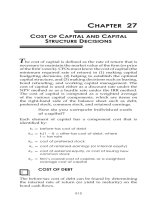
In Figure 17.1, we take a closer look at the effect of the proposed restructuring. This
figure plots earnings per share, EPS, against earnings before interest and taxes, EBIT, for
the current and proposed capital structures. The first line, labeled “No debt,” represents
the case of no leverage. This line begins at the origin, indicating that EPS would be zero
if EBIT were zero. From there, every $400,000 increase in EBIT increases EPS by $1
(because there are 400,000 shares outstanding).
The second line represents the proposed capital structure. Here, EPS is negative if EBIT
is zero. This follows because $400,000 of interest must be paid regardless of the firm’s
profits. Because there are 200,000 shares in this case, the EPS is Ϫ$2 as shown. Similarly,
if EBIT were $400,000, EPS would be exactly zero.
The important thing to notice in Figure 17.1 is that the slope of the line in this second
case is steeper. In fact, for every $400,000 increase in EBIT, EPS rises by $2, so the line
is twice as steep. This tells us that EPS is twice as sensitive to changes in EBIT because of
the financial leverage employed.

FIGURE 17.1
4
With debt

Earnings per share ($)

3

No debt

Financial Leverage:
EPS and EBIT for the
Trans Am Corporation

Advantage

to debt

2
Disadvantage
to debt

Break-even point

1

0

Ϫ1

400,000 800,000 1,200,000
Earnings before interest
and taxes ($, no taxes)

Ϫ2

ros3062x_Ch17.indd 555

2/8/07 3:00:05 PM


556

PA RT 6

Cost of Capital and Long-Term Financial Policy


Another observation to make in Figure 17.1 is that the lines intersect. At that point,
EPS is exactly the same for both capital structures. To find this point, note that EPS
is equal to EBIT͞400,000 in the no-debt case. In the with-debt case, EPS is (EBIT Ϫ
$400,000)͞200,000. If we set these equal to each other, EBIT is:
EBIT͞400,000 ϭ (EBIT Ϫ $400,000)͞200,000
EBIT ϭ 2 ϫ (EBIT Ϫ $400,000)
ϭ $800,000
When EBIT is $800,000, EPS is $2 under either capital structure. This is labeled as the
break-even point in Figure 17.1; we could also call it the indifference point. If EBIT is
above this level, leverage is beneficial; if it is below this point, it is not.
There is another, more intuitive, way of seeing why the break-even point is $800,000.
Notice that, if the firm has no debt and its EBIT is $800,000, its net income is also $800,000.
In this case, the ROE is 10 percent. This is precisely the same as the interest rate on the
debt, so the firm earns a return that is just sufficient to pay the interest.

EXAMPLE 17.1

Break-Even EBIT
The MPD Corporation has decided in favor of a capital restructuring. Currently, MPD uses
no debt financing. Following the restructuring, however, debt will be $1 million. The interest rate on the debt will be 9 percent. MPD currently has 200,000 shares outstanding,
and the price per share is $20. If the restructuring is expected to increase EPS, what is
the minimum level for EBIT that MPD’s management must be expecting? Ignore taxes in
answering.
To answer, we calculate the break-even EBIT. At any EBIT above this, the increased
financial leverage will increase EPS, so this will tell us the minimum level for EBIT. Under
the old capital structure, EPS is simply EBIT͞200,000. Under the new capital structure,
the interest expense will be $1 million ϫ .09 ϭ $90,000. Furthermore, with the $1 million
proceeds, MPD will repurchase $1 million͞20 ϭ 50,000 shares of stock, leaving 150,000
outstanding. EPS will thus be (EBIT Ϫ $90,000)͞150,000.

Now that we know how to calculate EPS under both scenarios, we set them equal to
each other and solve for the break-even EBIT:
EBIT͞200,000 ϭ (EBIT Ϫ $90,000)͞150,000
EBIT ϭ 4͞3 ϫ (EBIT Ϫ $90,000)
ϭ $360,000
Verify that, in either case, EPS is $1.80 when EBIT is $360,000. Management at MPD is
apparently of the opinion that EPS will exceed $1.80.

CORPORATE BORROWING AND HOMEMADE LEVERAGE
Based on Tables 17.3 and 17.4 and Figure 17.1, Ms. Morris draws the following conclusions:
1. The effect of financial leverage depends on the company’s EBIT. When EBIT is relatively high, leverage is beneficial.
2. Under the expected scenario, leverage increases the returns to shareholders, as measured
by both ROE and EPS.

ros3062x_Ch17.indd 556

2/8/07 3:00:05 PM


C H A P T E R 17

557

Financial Leverage and Capital Structure Policy

3. Shareholders are exposed to more risk under the proposed capital structure because
the EPS and ROE are much more sensitive to changes in EBIT in this case.
4. Because of the impact that financial leverage has on both the expected return
to stockholders and the riskiness of the stock, capital structure is an important
consideration.

The first three of these conclusions are clearly correct. Does the last conclusion necessarily follow? Surprisingly, the answer is no. As we discuss next, the reason is that
shareholders can adjust the amount of financial leverage by borrowing and lending on
their own. This use of personal borrowing to alter the degree of financial leverage is called
homemade leverage.
We will now illustrate that it actually makes no difference whether or not Trans Am
adopts the proposed capital structure, because any stockholder who prefers the proposed
capital structure can simply create it using homemade leverage. To begin, the first part
of Table 17.5 shows what will happen to an investor who buys $2,000 worth of Trans
Am stock if the proposed capital structure is adopted. This investor purchases 100 shares
of stock. From Table 17.4, we know that EPS will be $.50, $3, or $5.50, so the total
earnings for 100 shares will be either $50, $300, or $550 under the proposed capital
structure.
Now, suppose that Trans Am does not adopt the proposed capital structure. In this case,
EPS will be $1.25, $2.50, or $3.75. The second part of Table 17.5 demonstrates how a
stockholder who prefers the payoffs under the proposed structure can create them using
personal borrowing. To do this, the stockholder borrows $2,000 at 10 percent on her or
his own. Our investor uses this amount, along with the original $2,000, to buy 200 shares
of stock. As shown, the net payoffs are exactly the same as those for the proposed capital
structure.
How did we know to borrow $2,000 to create the right payoffs? We are trying to replicate Trans Am’s proposed capital structure at the personal level. The proposed capital
structure results in a debt– equity ratio of 1. To replicate this structure at the personal level,
the stockholder must borrow enough to create this same debt– equity ratio. Because the
stockholder has $2,000 in equity invested, the borrowing of another $2,000 will create a
personal debt– equity ratio of 1.
This example demonstrates that investors can always increase financial leverage themselves to create a different pattern of payoffs. It thus makes no difference whether Trans
Am chooses the proposed capital structure.

The use of personal
borrowing to change the
overall amount of financial

leverage to which the
individual is exposed.

TABLE 17.5

Proposed Capital Structure

EPS
Earnings for 100 shares
Net cost ϭ 100 shares ϫ $20 ϭ $2,000

homemade leverage

Recession

Expected

Expansion

$ .50
50.00

$ 3.00
300.00

$ 5.50
550.00

Proposed Capital
Structure versus Original

Capital Structure with
Homemade Leverage

Original Capital Structure and Homemade Leverage
EPS
$ 1.25
$ 2.50
Earnings for 200 shares
250.00
500.00
Less: Interest on $2,000 at 10%
200.00
200.00
Net earnings
$ 50.00
$300.00
Net cost ϭ 200 shares ϫ $20 Ϫ Amount borrowed ϭ $4,000 Ϫ 2,000 ϭ $2,000

ros3062x_Ch17.indd 557

$ 3.75
750.00
200.00
$550.00

2/8/07 3:00:06 PM


558


PA RT 6

EXAMPLE 17.2

Cost of Capital and Long-Term Financial Policy

Unlevering the Stock
In our Trans Am example, suppose management adopts the proposed capital structure.
Further suppose that an investor who owned 100 shares preferred the original capital structure. Show how this investor could “unlever” the stock to recreate the original payoffs.
To create leverage, investors borrow on their own. To undo leverage, investors must
lend money. In the case of Trans Am, the corporation borrowed an amount equal to half
its value. The investor can unlever the stock by simply lending money in the same proportion. In this case, the investor sells 50 shares for $1,000 total and then lends the $1,000 at
10 percent. The payoffs are calculated in the following table:
Recession
EPS (proposed structure)
Earnings for 50 shares
Plus: Interest on $1,000
Total payoff

Expected

Expansion

$ 3.00
150.00
100.00
$250.00

$ 5.50
275.00

100.00
$375.00

$

.50
25.00
100.00
$125.00

These are precisely the payoffs the investor would have experienced under the original
capital structure.

Concept Questions
17.2a What is the impact of financial leverage on stockholders?
17.2b What is homemade leverage?
17.2c Why is Trans Am’s capital structure irrelevant?

17.3 Capital Structure and

the Cost of Equity Capital

M&M Proposition I
The proposition that the
value of the firm is
independent of the firm’s
capital structure.

We have seen that there is nothing special about corporate borrowing because investors can
borrow or lend on their own. As a result, whichever capital structure Trans Am chooses,

the stock price will be the same. Trans Am’s capital structure is thus irrelevant, at least in
the simple world we have examined.
Our Trans Am example is based on a famous argument advanced by two Nobel laureates, Franco Modigliani and Merton Miller, whom we will henceforth call M&M. What
we illustrated for the Trans Am Corporation is a special case of M&M Proposition I.
M&M Proposition I states that it is completely irrelevant how a firm chooses to arrange its
finances.

M&M PROPOSITION I: THE PIE MODEL
One way to illustrate M&M Proposition I is to imagine two firms that are identical on the
left side of the balance sheet. Their assets and operations are exactly the same. The right
sides are different because the two firms finance their operations differently. In this case,
we can view the capital structure question in terms of a “pie” model. Why we choose this
name is apparent from Figure 17.2. Figure 17.2 gives two possible ways of cutting up the

ros3062x_Ch17.indd 558

2/8/07 3:00:07 PM


C H A P T E R 17

Value of firm

Stocks
40%

Bonds
60%

559


Financial Leverage and Capital Structure Policy

FIGURE 17.2

Value of firm

Stocks
60%

Two Pie Models of
Capital Structure

Bonds
40%

pie between the equity slice, E, and the debt slice, D: 40%–60% and 60%–40%. However,
the size of the pie in Figure 17.2 is the same for both firms because the value of the assets
is the same. This is precisely what M&M Proposition I states: The size of the pie doesn’t
depend on how it is sliced.

THE COST OF EQUITY AND FINANCIAL LEVERAGE: M&M PROPOSITION II
Although changing the capital structure of the firm does not change the firm’s total value,
it does cause important changes in the firm’s debt and equity. We now examine what happens to a firm financed with debt and equity when the debt– equity ratio is changed. To
simplify our analysis, we will continue to ignore taxes.
Based on our discussion in Chapter 15, if we ignore taxes, the weighted average cost of
capital, WACC, is:
WACC ϭ (E͞V) ϫ RE ϩ (D͞V) ϫ RD
where V ϭ E ϩ D. We also saw that one way of interpreting the WACC is as the required
return on the firm’s overall assets. To remind us of this, we will use the symbol RA to stand

for the WACC and write:
RA ϭ (E͞V) ϫ RE ϩ (D͞V) ϫ RD
If we rearrange this to solve for the cost of equity capital, we see that:
RE ϭ RA ϩ (RA Ϫ RD) ϫ (D͞E)

[17.1]

This is the famous M&M Proposition II, which tells us that the cost of equity depends on
three things: the required rate of return on the firm’s assets, RA; the firm’s cost of debt, RD;
and the firm’s debt– equity ratio, D͞E.
Figure 17.3 summarizes our discussion thus far by plotting the cost of equity capital,
RE , against the debt– equity ratio. As shown, M&M Proposition II indicates that the cost of
equity, RE , is given by a straight line with a slope of (RA Ϫ RD). The y-intercept corresponds
to a firm with a debt– equity ratio of zero, so RA ϭ RE in that case. Figure 17.3 shows that
as the firm raises its debt– equity ratio, the increase in leverage raises the risk of the equity
and therefore the required return or cost of equity (RE).
Notice in Figure 17.3 that the WACC doesn’t depend on the debt– equity ratio; it’s the
same no matter what the debt– equity ratio is. This is another way of stating M&M Proposition I: The firm’s overall cost of capital is unaffected by its capital structure. As illustrated,
the fact that the cost of debt is lower than the cost of equity is exactly offset by the increase
in the cost of equity from borrowing. In other words, the change in the capital structure
weights (E͞V and D͞V) is exactly offset by the change in the cost of equity (RE), so the
WACC stays the same.

ros3062x_Ch17.indd 559

M&M Proposition II
The proposition that a
firm’s cost of equity capital
is a positive linear
function of the firm’s capital

structure.

2/8/07 3:00:08 PM


560

PA RT 6

Cost of Capital and Long-Term Financial Policy

FIGURE 17.3
RE
Cost of capital (%)

The Cost of Equity
and the WACC: M&M
Propositions I and II with
No Taxes

WACC ϭ RA

RD

Debt–equity ratio (D/E)
RE ϭ RA ϩ (RA Ϫ RD) ϫ (D/E) by M&M Proposition II
E
D
RA ϭ WACC ϭ
ϫ RE ϩ

ϫ RD
V
V
where V ϭ D ϩ E

( (

EXAMPLE 17.3

( (

The Cost of Equity Capital
The Ricardo Corporation has a weighted average cost of capital (ignoring taxes) of 12 percent. It can borrow at 8 percent. Assuming that Ricardo has a target capital structure of
80 percent equity and 20 percent debt, what is its cost of equity? What is the cost of equity
if the target capital structure is 50 percent equity? Calculate the WACC using your answers
to verify that it is the same.
According to M&M Proposition II, the cost of equity, RE, is:
RE ϭ RA ϩ (RA Ϫ RD) ϫ (D͞E )
In the first case, the debt– equity ratio is .2͞.8 ϭ .25, so the cost of the equity is:
RE ϭ 12% ϩ (12% Ϫ 8%) ϫ .25
ϭ 13%
In the second case, verify that the debt– equity ratio is 1.0, so the cost of equity is
16 percent.
We can now calculate the WACC assuming that the percentage of equity financing is
80 percent, the cost of equity is 13 percent, and the tax rate is zero:
WACC ϭ (E͞V ) ϫ RE ϩ (D͞V ) ϫ RD
ϭ .80 ϫ 13% ϩ .20 ϫ 8%
ϭ 12%
In the second case, the percentage of equity financing is 50 percent and the cost of equity
is 16 percent. The WACC is:

WACC ϭ (E͞V ) ϫ RE ϩ (D͞V ) ϫ RD
ϭ .50 ϫ 16% ϩ .50 ϫ 8%
ϭ 12%
As we have calculated, the WACC is 12 percent in both cases.

ros3062x_Ch17.indd 560

2/8/07 3:00:08 PM


IN THEIR OWN WORDS . . .

C H A P T E R 17

561

Financial Leverage and Capital Structure Policy

Merton H. Miller on Capital Structure: M&M 30 Years Later
How difficult it is to summarize briefly the contribution of these papers was brought home to me very
clearly after Franco Modigliani was awarded the Nobel Prize in Economics, in part—but, of course, only in
part—for the work in finance. The television camera crews from our local stations in Chicago immediately
descended upon me. “We understand,” they said, “that you worked with Modigliani some years back in
developing these M&M theorems, and we wonder if you could explain them briefly to our television
viewers.” “How briefly?” I asked. “Oh, take 10 seconds,” was the reply.
Ten seconds to explain the work of a lifetime! Ten seconds to describe two carefully reasoned articles,
each running to more than 30 printed pages and each with 60 or so long footnotes! When they saw the look
of dismay on my face, they said, “You don’t have to go into details. Just give us the main points in simple,
commonsense terms.”
The main point of the cost-of-capital article was, in principle at least, simple enough to make. It said

that in an economist’s ideal world, the total market value of all the securities issued by a firm would be
governed by the earning power and risk of its underlying real assets and would be independent of how
the mix of securities issued to finance it was divided between debt instruments and equity capital. Some
corporate treasurers might well think that they could enhance total value by increasing the proportion of
debt instruments because yields on debt instruments, given their lower risk, are, by and large, substantially
below those on equity capital. But, under the ideal conditions assumed, the added risk to the shareholders
from issuing more debt will raise required yields on the equity by just enough to offset the seeming gain
from use of low-cost debt.
Such a summary would not only have been too long, but it relied on shorthand terms and concepts that
are rich in connotations to economists, but hardly so to the general public. I thought, instead, of an analogy
that we ourselves had invoked in the original paper. “Think of the firm,” I said, “as a gigantic tub of whole
milk. The farmer can sell the whole milk as is. Or he can separate out the cream and sell it at a considerably higher price than the whole milk would bring. (Selling cream is the analog of a firm selling low-yield
and hence high-priced debt securities.) But, of course, what the farmer would have left would be skim
milk, with low butterfat content, and that would sell for much less than whole milk. Skim milk corresponds
to the levered equity. The M&M proposition says that if there were no costs of separation (and, of course,
no government dairy support programs), the cream plus the skim milk would bring the same price as the
whole milk.”
The television people conferred among themselves for a while. They informed me that it was still too
long, too complicated, and too academic. “Have you anything simpler?” they asked. I thought of another
way in which the M&M proposition is presented that stresses the role of securities as devices for “partitioning” a firm’s payoffs among the group of its capital suppliers. “Think of the firm,” I said, “as a gigantic pizza,
divided into quarters. If, now, you cut each quarter in half into eighths, the M&M proposition says that you
will have more pieces, but not more pizza.”
Once again whispered conversation. This time, they shut the lights off. They folded up their equipment.
They thanked me for my cooperation. They said they would get back to me. But I knew that I had somehow
lost my chance to start a new career as a packager of economic wisdom for TV viewers in convenient
10-second sound bites. Some have the talent for it; and some just don’t.
The late Merton H. Miller was famous for his pathbreaking work with Franco Modigliani on corporate capital structure, cost of capital, and dividend policy.
He received the Nobel Prize in Economics for his contributions shortly after this essay was prepared.

BUSINESS AND FINANCIAL RISK

M&M Proposition II shows that the firm’s cost of equity can be broken down into two
components. The first component, RA, is the required return on the firm’s assets overall,
and it depends on the nature of the firm’s operating activities. The risk inherent in a firm’s
operations is called the business risk of the firm’s equity. Referring back to Chapter 13,
note that this business risk depends on the systematic risk of the firm’s assets. The greater a

business risk
The equity risk that comes
from the nature of the firm’s
operating activities.

561

ros3062x_Ch17.indd 561

2/8/07 3:00:11 PM


562

PA RT 6

financial risk

firm’s business risk, the greater RA will be, and, all other things being the same, the greater
will be the firm’s cost of equity.
The second component in the cost of equity, (RA Ϫ RD) ϫ (D͞E), is determined by the
firm’s financial structure. For an all-equity firm, this component is zero. As the firm begins
to rely on debt financing, the required return on equity rises. This occurs because the debt
financing increases the risks borne by the stockholders. This extra risk that arises from the

use of debt financing is called the financial risk of the firm’s equity.
The total systematic risk of the firm’s equity thus has two parts: business risk and financial risk. The first part (the business risk) depends on the firm’s assets and operations and
is not affected by capital structure. Given the firm’s business risk (and its cost of debt), the
second part (the financial risk) is completely determined by financial policy. As we have
illustrated, the firm’s cost of equity rises when the firm increases its use of financial leverage
because the financial risk of the equity increases while the business risk remains the same.

The equity risk that comes
from the financial policy
(the capital structure) of
the firm.

Cost of Capital and Long-Term Financial Policy

Concept Questions
17.3a What does M&M Proposition I state?
17.3b What are the three determinants of a firm’s cost of equity?
17.3c The total systematic risk of a firm’s equity has two parts. What are they?

17.4 M&M Propositions I and II

with Corporate Taxes
Debt has two distinguishing features that we have not taken into proper account. First, as
we have mentioned in a number of places, interest paid on debt is tax deductible. This is
good for the firm, and it may be an added benefit of debt financing. Second, failure to meet
debt obligations can result in bankruptcy. This is not good for the firm, and it may be an
added cost of debt financing. Because we haven’t explicitly considered either of these two
features of debt, we realize that we may get a different answer about capital structure once
we do. Accordingly, we consider taxes in this section and bankruptcy in the next one.
We can start by considering what happens to M&M Propositions I and II when we

consider the effect of corporate taxes. To do this, we will examine two firms: Firm U (unlevered) and Firm L (levered). These two firms are identical on the left side of the balance
sheet, so their assets and operations are the same.
We assume that EBIT is expected to be $1,000 every year forever for both firms. The
difference between the firms is that Firm L has issued $1,000 worth of perpetual bonds
on which it pays 8 percent interest each year. The interest bill is thus .08 ϫ $1,000 ϭ $80
every year forever. Also, we assume that the corporate tax rate is 30 percent.
For our two firms, U and L, we can now calculate the following:

EBIT
Interest
Taxable income
Taxes (30%)
Net income

ros3062x_Ch17.indd 562

Firm U

Firm L

$1,000
0
$1,000
300
$ 700

$1,000
80
$ 920
276

$ 644

2/8/07 3:00:13 PM


C H A P T E R 17

563

Financial Leverage and Capital Structure Policy

THE INTEREST TAX SHIELD
To simplify things, we will assume that depreciation is zero. We will also assume that
capital spending is zero and that there are no changes in NWC. In this case, cash flow from
assets is simply equal to EBIT Ϫ Taxes. For Firms U and L, we thus have:
Cash Flow from Assets
EBIT
Ϫ Taxes
Total

Firm U

Firm L

$1,000
300
$ 700

$1,000
276

$ 724

We immediately see that capital structure is now having some effect because the cash
flows from U and L are not the same even though the two firms have identical assets.
To see what’s going on, we can compute the cash flow to stockholders and bondholders:
Cash Flow
To stockholders
To bondholders
Total

Firm U

Firm L

$700
0
$700

$644
80
$724

What we are seeing is that the total cash flow to L is $24 more. This occurs because L’s tax
bill (which is a cash outflow) is $24 less. The fact that interest is deductible for tax purposes
has generated a tax saving equal to the interest payment ($80) multiplied by the corporate
tax rate (30 percent): $80 ϫ .30 ϭ $24. We call this tax saving the interest tax shield.

interest tax shield

TAXES AND M&M PROPOSITION I


The tax saving attained
by a firm from interest
expense.

Because the debt is perpetual, the same $24 shield will be generated every year forever.
The aftertax cash flow to L will thus be the same $700 that U earns plus the $24 tax shield.
Because L’s cash flow is always $24 greater, Firm L is worth more than Firm U, the difference being the value of this $24 perpetuity.
Because the tax shield is generated by paying interest, it has the same risk as the debt,
and 8 percent (the cost of debt) is therefore the appropriate discount rate. The value of the
tax shield is thus:
$24 .30 ϫ $1,000 ϫ .08
PV ϭ ____ ϭ ________________ ϭ .30($1,000) ϭ $300
.08
.08
As our example illustrates, the present value of the interest tax shield can be written as:
Present value of the interest tax shield ϭ (TC ϫ D ϫ RD)͞RD
ϭ TC ϫ D

[17.2]

We have now come up with another famous result, M&M Proposition I with corporate
taxes. We have seen that the value of Firm L, VL, exceeds the value of Firm U, VU, by
the present value of the interest tax shield, TC ϫ D. M&M Proposition I with taxes therefore states that:
VL ϭ VU ϩ TC ϫ D

[17.3]

The effect of borrowing in this case is illustrated in Figure 17.4. We have plotted the
value of the levered firm, VL, against the amount of debt, D. M&M Proposition I with

corporate taxes implies that the relationship is given by a straight line with a slope of TC
and a y-intercept of VU.

ros3062x_Ch17.indd 563

2/8/07 3:00:14 PM


564

PA RT 6

Cost of Capital and Long-Term Financial Policy

FIGURE 17.4

V L ϭ V U ϩ TC ϫ D

M&M Proposition I with
Taxes
Value of the firm (VL)

ϭ TC

TC ϫ D

VL ϭ $7,300
VU ϭ $7,000

VU


VU

1,000
Total debt (D)
The value of the firm increases as total debt increases because of the interest tax shield.
This is the basis of M&M Proposition I with taxes.

unlevered cost of
capital
The cost of capital for a
firm that has no debt.

In Figure 17.4, we have also drawn a horizontal line representing VU. As indicated, the
distance between the two lines is TC ϫ D, the present value of the tax shield.
Suppose that the cost of capital for Firm U is 10 percent. We will call this the unlevered
cost of capital, and we will use the symbol RU to represent it. We can think of RU as the
cost of capital a firm would have if it had no debt. Firm U’s cash flow is $700 every year
forever, and, because U has no debt, the appropriate discount rate is RU ϭ 10%. The value
of the unlevered firm, VU, is simply:
EBIT ϫ (1 Ϫ TC)
VU ϭ _______________
RU
$700
ϭ _____
.10
ϭ $7,000
The value of the levered firm, VL, is:
VL ϭ VU ϩ TC ϫ D
ϭ $7,000 ϩ .30 ϫ 1,000

ϭ $7,300
As Figure 17.4 indicates, the value of the firm goes up by $.30 for every $1 in debt. In
other words, the NPV per dollar of debt is $.30. It is difficult to imagine why any corporation would not borrow to the absolute maximum under these circumstances.
The result of our analysis in this section is the realization that, once we include taxes,
capital structure definitely matters. However, we immediately reach the illogical conclusion that the optimal capital structure is 100 percent debt.

TAXES, THE WACC, AND PROPOSITION II
We can also conclude that the best capital structure is 100 percent debt by examining the
weighted average cost of capital. From Chapter 15, we know that once we consider the

ros3062x_Ch17.indd 564

2/8/07 3:00:14 PM


C H A P T E R 17

565

Financial Leverage and Capital Structure Policy

effect of taxes, the WACC is:
WACC ϭ (E͞V) ϫ RE ϩ (D͞V) ϫ RD ϫ (1 Ϫ TC)
To calculate this WACC, we need to know the cost of equity. M&M Proposition II with
corporate taxes states that the cost of equity is:
RE ϭ RU ϩ (RU Ϫ RD ) ϫ (D͞E ) ϫ (1 Ϫ TC )

[17.4]

To illustrate, recall that we saw a moment ago that Firm L is worth $7,300 total. Because

the debt is worth $1,000, the equity must be worth $7,300 Ϫ 1,000 ϭ $6,300. For Firm L,
the cost of equity is thus:
RE ϭ .10 ϩ (.10 Ϫ .08) ϫ ($1,000͞6,300) ϫ (1 Ϫ .30)
ϭ 10.22%
The weighted average cost of capital is:
WACC ϭ ($6,300͞7,300) ϫ 10.22% ϩ (1,000͞7,300) ϫ 8% ϫ (1 Ϫ .30)
ϭ 9.6%
Without debt, the WACC is over 10 percent; with debt, it is 9.6 percent. Therefore, the firm
is better off with debt.

CONCLUSION
Figure 17.5 summarizes our discussion concerning the relationship between the cost of
equity, the aftertax cost of debt, and the weighted average cost of capital. For reference, we
FIGURE 17.5

Cost of capital (%)

RE

The Cost of Equity
and the WACC: M&M
Proposition II with Taxes

RE ϭ 10.22%

RU ϭ 10%

RU

WACC ϭ 9.6%

WACC
RD ϫ (1 Ϫ TC)

RD ϫ (1 Ϫ TC)
ϭ 8% ϫ (1 Ϫ .30)
ϭ 5.6%
$1,000/6,300 ϭ D/E
Debt–equity ratio (D/E)

M&M Proposition I with taxes implies that a firm’s WACC decreases
as the firm relies more heavily on debt financing:
E
D
WACC ϭ
ϫ RE ϩ
ϫ RD ϫ (1 Ϫ TC)
V
V

( (

( (

M&M Proposition II with taxes implies that a firm’s cost of equity,
RE, rises as the firm relies more heavily on debt financing:
RE ϭ RU ϩ (RU Ϫ RD) ϫ (D/E) ϫ (1 Ϫ TC)

ros3062x_Ch17.indd 565

2/8/07 3:00:15 PM



566

PA RT 6

Cost of Capital and Long-Term Financial Policy

have included RU, the unlevered cost of capital. In Figure 17.5, we have the debt– equity
ratio on the horizontal axis. Notice how the WACC declines as the debt– equity ratio grows.
This illustrates again that the more debt the firm uses, the lower is its WACC. Table 17.6
summarizes the key results of our analysis of the M&M propositions for future reference.
TABLE 17.6

I.

The No-Tax Case
A. Proposition I: The value of the firm levered (VL) is equal to the value of the firm unlevered (VU ):

Modigliani and Miller
Summary

VL ϭ VU
Implications of Proposition I:
1. A firm’s capital structure is irrelevant.
2. A firm’s weighted average cost of capital (WACC) is the same no matter what mixture
of debt and equity is used to finance the firm.
B. Proposition II: The cost of equity, RE, is:
RE ϭ RA ϩ (RA Ϫ RD ) ϫ (D͞E)
where RA is the WACC, RD is the cost of debt, and D͞E is the debt– equity ratio.

Implications of Proposition II:
1. The cost of equity rises as the firm increases its use of debt financing.
2. The risk of the equity depends on two things: the riskiness of the firm’s operations
(business risk) and the degree of financial leverage (financial risk). Business risk determines RA; financial risk is determined by D͞E.
II.

The Tax Case
A. Proposition I with taxes: The value of the firm levered (VL) is equal to the value of the
firm unlevered (VU) plus the present value of the interest tax shield:
VL ϭ VU ϩ TC ϫ D
where TC is the corporate tax rate and D is the amount of debt.
Implications of Proposition I:
1. Debt financing is highly advantageous, and, in the extreme, a firm’s optimal capital
structure is 100 percent debt.
2. A firm’s weighted average cost of capital (WACC) decreases as the firm relies more
heavily on debt financing.
B. Proposition II with taxes: The cost of equity, RE, is:
RE ϭ RU ϩ (RU Ϫ RD ) ϫ (D͞E) ϫ (1 Ϫ TC)
where RU is the unlevered cost of capital—that is, the cost of capital for the firm if it has no
debt. Unlike the case with Proposition I, the general implications of Proposition II are the
same whether there are taxes or not.

EXAMPLE 17.4

The Cost of Equity and the Value of the Firm
This is a comprehensive example that illustrates most of the points we have discussed
thus far. You are given the following information for the Format Co.:
EBIT ϭ $151.52
TC ϭ .34
D ϭ $500

RU ϭ .20
The cost of debt capital is 10 percent. What is the value of Format’s equity? What is the
cost of equity capital for Format? What is the WACC?
(continued)

ros3062x_Ch17.indd 566

2/8/07 3:00:15 PM


C H A P T E R 17

567

Financial Leverage and Capital Structure Policy

This one’s easier than it looks. Remember that all the cash flows are perpetuities. The
value of the firm if it has no debt, VU, is:
EBIT Ϫ Taxes EBIT ϫ (1 Ϫ TC)
VU ϭ _____________ ϭ _______________
RU
RU
$100
ϭ _____
.20
ϭ $500
From M&M Proposition I with taxes, we know that the value of the firm with debt is:
VL ϭ VU ϩ TC ϫ D
ϭ $500 ϩ .34 ϫ 500
ϭ $670

Because the firm is worth $670 total and the debt is worth $500, the equity is worth $170:
E ϭ VL Ϫ D
ϭ $670 Ϫ 500
ϭ $170
Based on M&M Proposition II with taxes, the cost of equity is:
RE ϭ RU ϩ (RU Ϫ RD) ϫ (D͞E) ϫ (1 Ϫ TC)
ϭ .20 ϩ (.20 Ϫ .10) ϫ ($500͞170) ϫ (1 Ϫ .34)
ϭ 39.4%
Finally, the WACC is:
WACC ϭ ($170͞670) ϫ 39.4% ϩ (500͞670) ϫ 10% ϫ (1 Ϫ .34)
ϭ 14.92%
Notice that this is substantially lower than the cost of capital for the firm with no debt
(RU ϭ 20%), so debt financing is highly advantageous.

Concept Questions
17.4a What is the relationship between the value of an unlevered firm and the value
of a levered firm once we consider the effect of corporate taxes?
17.4b If we consider only the effect of taxes, what is the optimal capital structure?

Bankruptcy Costs

17.5

One limiting factor affecting the amount of debt a firm might use comes in the form
of bankruptcy costs. As the debt– equity ratio rises, so too does the probability that the
firm will be unable to pay its bondholders what was promised to them. When this happens, ownership of the firm’s assets is ultimately transferred from the stockholders to
the bondholders.
In principle, a firm becomes bankrupt when the value of its assets equals the value of its
debt. When this occurs, the value of equity is zero, and the stockholders turn over control


ros3062x_Ch17.indd 567

2/8/07 3:00:17 PM


568

PA RT 6

Cost of Capital and Long-Term Financial Policy

of the firm to the bondholders. When this takes place, the bondholders hold assets whose
value is exactly equal to what is owed on the debt. In a perfect world, there are no costs
associated with this transfer of ownership, and the bondholders don’t lose anything.
This idealized view of bankruptcy is not, of course, what happens in the real world.
Ironically, it is expensive to go bankrupt. As we discuss, the costs associated with bankruptcy may eventually offset the tax-related gains from leverage.

DIRECT BANKRUPTCY COSTS

direct bankruptcy
costs
The costs that are
directly associated with
bankruptcy, such as
legal and administrative
expenses.

When the value of a firm’s assets equals the value of its debt, then the firm is economically bankrupt in the sense that the equity has no value. However, the formal turning over
of the assets to the bondholders is a legal process, not an economic one. There are legal
and administrative costs to bankruptcy, and it has been remarked that bankruptcies are to

lawyers what blood is to sharks.
For example, in December 2001, energy products giant Enron filed for bankruptcy in
the largest U.S. bankruptcy to date. Over the next three years, the company went through
the bankruptcy process, finally emerging in November 2004. The direct bankruptcy costs
were staggering: Enron spent over $1 billion on lawyers, accountants, consultants, and
examiners, and the final tally may be higher. Other recent expensive bankruptcies include
WorldCom ($600 million), Adelphia Communications ($370 million), and United Airlines
($335 million).
Because of the expenses associated with bankruptcy, bondholders won’t get all that they
are owed. Some fraction of the firm’s assets will “disappear” in the legal process of going
bankrupt. These are the legal and administrative expenses associated with the bankruptcy
proceeding. We call these costs direct bankruptcy costs.
These direct bankruptcy costs are a disincentive to debt financing. If a firm goes bankrupt, then, suddenly, a piece of the firm disappears. This amounts to a bankruptcy “tax.” So
a firm faces a trade-off: Borrowing saves a firm money on its corporate taxes, but the more
a firm borrows, the more likely it is that the firm will become bankrupt and have to pay the
bankruptcy tax.

INDIRECT BANKRUPTCY COSTS

indirect bankruptcy
costs
The costs of avoiding a
bankruptcy filing incurred
by a financially distressed
firm.

financial distress costs
The direct and indirect
costs associated with going
bankrupt or experiencing

financial distress.

ros3062x_Ch17.indd 568

Because it is expensive to go bankrupt, a firm will spend resources to avoid doing so. When
a firm is having significant problems in meeting its debt obligations, we say that it is experiencing financial distress. Some financially distressed firms ultimately file for bankruptcy,
but most do not because they are able to recover or otherwise survive.
The costs of avoiding a bankruptcy filing incurred by a financially distressed firm
are called indirect bankruptcy costs. We use the term financial distress costs to refer
generically to the direct and indirect costs associated with going bankrupt or avoiding a
bankruptcy filing.
The problems that come up in financial distress are particularly severe, and the financial distress costs are thus larger, when the stockholders and the bondholders are different
groups. Until the firm is legally bankrupt, the stockholders control it. They, of course, will
take actions in their own economic interests. Because the stockholders can be wiped out in
a legal bankruptcy, they have a very strong incentive to avoid a bankruptcy filing.
The bondholders, on the other hand, are primarily concerned with protecting the value
of the firm’s assets and will try to take control away from stockholders. They have a strong
incentive to seek bankruptcy to protect their interests and keep stockholders from further
dissipating the assets of the firm. The net effect of all this fighting is that a long, drawn-out,
and potentially quite expensive legal battle gets started.

2/8/07 3:00:18 PM


C H A P T E R 17

569

Financial Leverage and Capital Structure Policy


Meanwhile, as the wheels of justice turn in their ponderous way, the assets of the firm
lose value because management is busy trying to avoid bankruptcy instead of running the
business. Normal operations are disrupted, and sales are lost. Valuable employees leave,
potentially fruitful programs are dropped to preserve cash, and otherwise profitable investments are not taken.
For example, in 2006, both General Motors and Ford were experiencing significant
financial difficulty, and many people felt that one or both companies would eventually file
for bankruptcy. As a result of the bad news surrounding both companies, there was a loss of
confidence in the companies’ automobiles. A study showed that 75 percent of Americans
would not purchase an automobile from a bankrupt company because the company might
not honor the warranty and it might be difficult to obtain replacement parts. This concern
resulted in lost potential sales for both companies, which only added to their financial
distress.
These are all indirect bankruptcy costs, or costs of financial distress. Whether or not the
firm ultimately goes bankrupt, the net effect is a loss of value because the firm chose to use
debt in its capital structure. It is this possibility of loss that limits the amount of debt that a
firm will choose to use.

Concept Questions
17.5a What are direct bankruptcy costs?
17.5b What are indirect bankruptcy costs?

Optimal Capital Structure

17.6

Our previous two sections have established the basis for determining an optimal capital
structure. A firm will borrow because the interest tax shield is valuable. At relatively low
debt levels, the probability of bankruptcy and financial distress is low, and the benefit from
debt outweighs the cost. At very high debt levels, the possibility of financial distress is a
chronic, ongoing problem for the firm, so the benefit from debt financing may be more

than offset by the financial distress costs. Based on our discussion, it would appear that an
optimal capital structure exists somewhere in between these extremes.

THE STATIC THEORY OF CAPITAL STRUCTURE
The theory of capital structure that we have outlined is called the static theory of capital
structure. It says that firms borrow up to the point where the tax benefit from an extra
dollar in debt is exactly equal to the cost that comes from the increased probability
of financial distress. We call this the static theory because it assumes that the firm is
fixed in terms of its assets and operations and it considers only possible changes in the
debt– equity ratio.
The static theory is illustrated in Figure 17.6, which plots the value of the firm, VL,
against the amount of debt, D. In Figure 17.6, we have drawn lines corresponding to three
different stories. The first represents M&M Proposition I with no taxes. This is the horizontal line extending from VU, and it indicates that the value of the firm is unaffected by its
capital structure. The second case, M&M Proposition I with corporate taxes, is represented
by the upward-sloping straight line. These two cases are exactly the same as the ones we
previously illustrated in Figure 17.4.

ros3062x_Ch17.indd 569

static theory of capital
structure
The theory that a firm
borrows up to the point
where the tax benefit
from an extra dollar in
debt is exactly equal to
the cost that comes from
the increased probability
of financial distress.


2/8/07 3:00:18 PM


570

PA RT 6

Cost of Capital and Long-Term Financial Policy

FIGURE 17.6
VL ϭ VU ϩ TC ϫ D
Present value of
tax shield on debt
Value of the firm (VL)

The Static Theory of
Capital Structure: The
Optimal Capital Structure
and the Value of the Firm

Financial distress
costs

Maximum
firm value VL*
Actual firm value
VU ϭ Value of firm
with no debt

VU


D*
Optimal amount of debt
Total debt (D)
According to the static theory, the gain from the tax shield on debt is offset by financial
distress costs. An optimal capital structure exists that just balances the additional gain
from leverage against the added financial distress cost.

The third case in Figure 17.6 illustrates our current discussion: The value of the firm
rises to a maximum and then declines beyond that point. This is the picture that we get
from our static theory. The maximum value of the firm, VL*, is reached at D*, so this point
represents the optimal amount of borrowing. Put another way, the firm’s optimal capital
structure is composed of D*͞VL* in debt and (1 Ϫ D*͞VL*) in equity.
The final thing to notice in Figure 17.6 is that the difference between the value of the
firm in our static theory and the M&M value of the firm with taxes is the loss in value
from the possibility of financial distress. Also, the difference between the static theory
value of the firm and the M&M value with no taxes is the gain from leverage, net of
distress costs.

OPTIMAL CAPITAL STRUCTURE AND THE COST OF CAPITAL
As we discussed earlier, the capital structure that maximizes the value of the firm is also
the one that minimizes the cost of capital. Figure 17.7 illustrates the static theory of capital
structure in terms of the weighted average cost of capital and the costs of debt and equity.
Notice in Figure 17.7 that we have plotted the various capital costs against the debt– equity
ratio, D͞E.
Figure 17.7 is much the same as Figure 17.5 except that we have added a new line for
the WACC. This line, which corresponds to the static theory, declines at first. This occurs
because the aftertax cost of debt is cheaper than equity, so, at least initially, the overall cost
of capital declines.
At some point, the cost of debt begins to rise, and the fact that debt is cheaper than

equity is more than offset by the financial distress costs. From this point, further increases
in debt actually increase the WACC. As illustrated, the minimum WACC* occurs at the
point D*րE*, just as we described before.

ros3062x_Ch17.indd 570

2/8/07 3:00:19 PM


C H A P T E R 17

571

Financial Leverage and Capital Structure Policy

FIGURE 17.7

Cost of capital (%)

RE

The Static Theory of
Capital Structure: The
Optimal Capital Structure
and the Cost of Capital

RU
WACC
RD ϫ (1 Ϫ TC )


RU
Minimum
cost of
WACC*
capital

D*/E*
Optimal
debt–equity ratio
Debt–equity ratio (D/E)
According to the static theory, the WACC falls initially because of the tax
advantage of debt. Beyond the point D*/E*, it begins to rise because of
financial distress costs.

OPTIMAL CAPITAL STRUCTURE: A RECAP
With the help of Figure 17.8, we can recap (no pun intended) our discussion of capital
structure and cost of capital. As we have noted, there are essentially three cases. We will
use the simplest of the three cases as a starting point and then build up to the static theory of
capital structure. Along the way, we will pay particular attention to the connection between
capital structure, firm value, and cost of capital.
Figure 17.8 presents the original Modigliani and Miller no-tax, no-bankruptcy argument
as Case I. This is the most basic case. In the top part of the figure, we have plotted the value
of the firm, VL, against total debt, D. When there are no taxes, bankruptcy costs, or other
real-world imperfections, we know that the total value of the firm is not affected by its debt
policy, so VL is simply constant. The bottom part of Figure 17.8 tells the same story in terms
of the cost of capital. Here, the weighted average cost of capital, WACC, is plotted against
the debt– equity ratio, D͞E. As with total firm value, the overall cost of capital is not affected
by debt policy in this basic case, so the WACC is constant.
Next, we consider what happens to the original M&M argument once taxes are introduced. As Case II illustrates, we now see that the firm’s value critically depends on its debt
policy. The more the firm borrows, the more it is worth. From our earlier discussion, we

know this happens because interest payments are tax deductible, and the gain in firm value
is just equal to the present value of the interest tax shield.
In the bottom part of Figure 17.8, notice how the WACC declines as the firm uses more
and more debt financing. As the firm increases its financial leverage, the cost of equity
does increase; but this increase is more than offset by the tax break associated with debt
financing. As a result, the firm’s overall cost of capital declines.
To finish our story, we include the impact of bankruptcy or financial distress costs to get
Case III. As shown in the top part of Figure 17.8, the value of the firm will not be as large
as we previously indicated. The reason is that the firm’s value is reduced by the present

ros3062x_Ch17.indd 571

2/8/07 3:00:19 PM


572

PA RT 6

Cost of Capital and Long-Term Financial Policy

FIGURE 17.8
Case II
M&M
(with taxes)

The Capital Structure
Question

Value of the firm (VL)


PV of bankruptcy
costs
VL*
Case III
Static theory
Net gain from leverage
Case I
M&M
(no taxes)

VU

D*

Weighted average cost of capital (%)

Total debt (D)

RU
Net saving from
leverage

Case I
M&M
(no taxes)
Case III
Static theory

WACC*

Case II
M&M
(with taxes)
D*/E*
Debt–equity ratio (D/E)

Case I
With no taxes or bankruptcy costs, the value of the firm and its weighted average cost of
capital are not affected by capital structures.
Case II
With corporate taxes and no bankruptcy costs, the value of the firm increases and the
weighted average cost of capital decreases as the amount of debt goes up.
Case III
With corporate taxes and bankruptcy costs, the value of the firm, VL, reaches a maximum
at D*, the point representing the optimal amount of borrowing. At the same time, the
weighted average cost of capital, WACC, is minimized at D*/E*.

ros3062x_Ch17.indd 572

2/8/07 3:00:20 PM


C H A P T E R 17

573

Financial Leverage and Capital Structure Policy

value of the potential future bankruptcy costs. These costs grow as the firm borrows more
and more, and they eventually overwhelm the tax advantage of debt financing. The optimal

capital structure occurs at D*, the point at which the tax saving from an additional dollar
in debt financing is exactly balanced by the increased bankruptcy costs associated with the
additional borrowing. This is the essence of the static theory of capital structure.
The bottom part of Figure 17.8 presents the optimal capital structure in terms of the cost
of capital. Corresponding to D*, the optimal debt level, is the optimal debt– equity ratio,
D*րE*. At this level of debt financing, the lowest possible weighted average cost of capital,
WACC*, occurs.

CAPITAL STRUCTURE: SOME MANAGERIAL RECOMMENDATIONS
The static model that we have described is not capable of identifying a precise optimal
capital structure, but it does point out two of the more relevant factors: taxes and financial
distress. We can draw some limited conclusions concerning these.

Taxes First of all, the tax benefit from leverage is obviously important only to firms that
are in a tax-paying position. Firms with substantial accumulated losses will get little value
from the interest tax shield. Furthermore, firms that have substantial tax shields from other
sources, such as depreciation, will get less benefit from leverage.
Also, not all firms have the same tax rate. The higher the tax rate, the greater the incentive to borrow.
Financial Distress Firms with a greater risk of experiencing financial distress will borrow less than firms with a lower risk of financial distress. For example, all other things
being equal, the greater the volatility in EBIT, the less a firm should borrow.
In addition, financial distress is more costly for some firms than others. The costs of
financial distress depend primarily on the firm’s assets. In particular, financial distress
costs will be determined by how easily ownership of those assets can be transferred.
For example, a firm with mostly tangible assets that can be sold without great loss in
value will have an incentive to borrow more. For firms that rely heavily on intangibles,
such as employee talent or growth opportunities, debt will be less attractive because these
assets effectively cannot be sold.

Concept Questions
17.6a Can you describe the trade-off that defines the static theory of capital structure?

17.6b What are the important factors in making capital structure decisions?

The Pie Again

17.7

Although it is comforting to know that the firm might have an optimal capital structure
when we take account of such real-world matters as taxes and financial distress costs, it is
disquieting to see the elegant original M&M intuition (that is, the no-tax version) fall apart
in the face of these matters.
Critics of the M&M theory often say that it fails to hold as soon as we add in real-world
issues and that the M&M theory is really just that: a theory that doesn’t have much to say
about the real world that we live in. In fact, they would argue that it is the M&M theory

ros3062x_Ch17.indd 573

2/8/07 3:00:20 PM


574

PA RT 6

Cost of Capital and Long-Term Financial Policy

that is irrelevant, not capital structure. As we discuss next, however, taking that view blinds
critics to the real value of the M&M theory.

THE EXTENDED PIE MODEL
To illustrate the value of the original M&M intuition, we briefly consider an expanded version of the pie model that we introduced earlier. In the extended pie model, taxes just represent another claim on the cash flows of the firm. Because taxes are reduced as leverage

is increased, the value of the government’s claim (G) on the firm’s cash flows decreases
with leverage.
Bankruptcy costs are also a claim on the cash flows. They come into play as the firm
comes close to bankruptcy and has to alter its behavior to attempt to stave off the event
itself, and they become large when bankruptcy actually takes place. Thus, the value of this
claim (B) on the cash flows rises with the debt– equity ratio.
The extended pie theory simply holds that all of these claims can be paid from only one
source: the cash flows (CF) of the firm. Algebraically, we must have:
CF ϭ Payments to stockholders ϩ Payments to creditors
ϩ Payments to the government
ϩ Payments to bankruptcy courts and lawyers
ϩ Payments to any and all other claimants to the cash flows of the firm
The extended pie model is illustrated in Figure 17.9. Notice that we have added a few slices
for the additional groups. Notice also the change in the relative sizes of the slices as the
firm’s use of debt financing is increased.
With the list we have developed, we have not even begun to exhaust the potential claims
to the firm’s cash flows. To give an unusual example, we might say that everyone reading
this book has an economic claim on the cash flows of General Motors. After all, if you are
injured in an accident, you might sue GM, and, win or lose, GM will expend some of its
cash flow in dealing with the matter. For GM, or any other company, there should thus be
a slice of the pie representing potential lawsuits. This is the essence of the M&M intuition

FIGURE 17.9
The Extended
Pie Model

Lower financial leverage

Bondholder
claim

Stockholder
claim

Bankruptcy
claim
Tax
claim

Higher financial leverage

Bondholder
claim

Stockholder
claim

Bankruptcy
claim
Tax
claim

In the extended pie model, the value of all the claims against the firm’s cash
flows is not affected by capital structure, but the relative values of claims
change as the amount of debt financing is increased.

ros3062x_Ch17.indd 574

2/8/07 3:00:21 PM



C H A P T E R 17

575

Financial Leverage and Capital Structure Policy

and theory: The value of the firm depends on the total cash flow of the firm. The firm’s
capital structure just cuts that cash flow up into slices without altering the total. What we
recognize now is that the stockholders and the bondholders may not be the only ones who
can claim a slice.

MARKETED CLAIMS VERSUS NONMARKETED CLAIMS
With our extended pie model, there is an important distinction between claims such as
those of stockholders and bondholders, on the one hand, and those of the government and
potential litigants in lawsuits on the other. The first set of claims are marketed claims, and
the second set are nonmarketed claims. A key difference is that the marketed claims can be
bought and sold in financial markets and the nonmarketed claims cannot.
When we speak of the value of the firm, we are generally referring to just the value of
the marketed claims, VM, and not the value of the nonmarketed claims, VN. If we write VT for
the total value of all the claims against a corporation’s cash flows, then:
VT ϭ E ϩ D ϩ G ϩ B ϩ . . .
ϭ VM ϩ VN
The essence of our extended pie model is that this total value, VT , of all the claims to the
firm’s cash flows is unaltered by capital structure. However, the value of the marketed
claims, VM, may be affected by changes in the capital structure.
Based on the pie theory, any increase in VM must imply an identical decrease in VN.
The optimal capital structure is thus the one that maximizes the value of the marketed
claims or, equivalently, minimizes the value of nonmarketed claims such as taxes and bankruptcy costs.

Concept Questions

17.7a What are some of the claims to a firm’s cash flows?
17.7b What is the difference between a marketed claim and a nonmarketed claim?
17.7c What does the extended pie model say about the value of all the claims to a
firm’s cash flows?

The Pecking-Order Theory

17.8

The static theory we have developed in this chapter has dominated thinking about capital
structure for a long time, but it has some shortcomings. Perhaps the most obvious is that
many large, financially sophisticated, and highly profitable firms use little debt. This is the
opposite of what we would expect. Under the static theory, these are the firms that should
use the most debt because there is little risk of bankruptcy and the value of the tax shield is
substantial. Why do they use so little debt? The pecking-order theory, which we consider
next, may be part of the answer.

INTERNAL FINANCING AND THE PECKING ORDER
The pecking-order theory is an alternative to the static theory. A key element in the peckingorder theory is that firms prefer to use internal financing whenever possible. A simple reason
is that selling securities to raise cash can be expensive, so it makes sense to avoid doing so if

ros3062x_Ch17.indd 575

2/8/07 3:00:21 PM