Eastman Chemical is a leading international chemical

which Eastman’s return on capital for the year exceeds

company and maker of plastics such as that used in

its cost of capital. With this approach, Eastman joined

soft drink containers. It was created on December

the many firms that tie compensation packages to

31, 1993, when its former parent company, Eastman

how good a job the firm does in providing an adequate

Kodak, split off the division as a separate company.

return for its investors. In this chapter, we learn how

Soon thereafter, Eastman Chemical adopted a new

to compute a firm’s cost of capital and find out what

motivational program for its employees. Everyone who

it means to the

works for the company, from hourly workers up to the

firm and its

CEO, gets a bonus that depends on the amount by

investors.

Visit us at www.mhhe.com/rwj
DIGITAL STUDY TOOLS
• Self-Study Software
• Multiple-Choice Quizzes
• Flashcards for Testing and
Key Terms

Suppose you have just become the president of a large company, and the first
decision you face is whether to go ahead with a plan to renovate the company’s
warehouse distribution system. The plan will cost the company $50 million,
and it is expected to save $12 million per year after taxes over the next six years.
This is a familiar problem in capital budgeting. To address it, you would determine the
relevant cash flows, discount them, and, if the net present value is positive, take on the
project; if the NPV is negative, you would scrap it. So far, so good; but what should you
use as the discount rate?
From our discussion of risk and return, you know that the correct discount rate depends
on the riskiness of the project to renovate the warehouse distribution system. In particular,
the new project will have a positive NPV only if its return exceeds what the financial markets offer on investments of similar risk. We called this minimum required return the cost
of capital associated with the project.1
Thus, to make the right decision as president, you must examine what the capital markets
have to offer and use this information to arrive at an estimate of the project’s cost of capital.
Our primary purpose in this chapter is to describe how to go about doing this. There are a
variety of approaches to this task, and a number of conceptual and practical issues arise.
One of the most important concepts we develop is that of the weighted average cost of
capital (WACC). This is the cost of capital for the firm as a whole, and it can be interpreted

as the required return on the overall firm. In discussing the WACC, we will recognize the
fact that a firm will normally raise capital in a variety of forms and that these different
forms of capital may have different costs associated with them.

Cost of Capital and Long-Term
Capital
Financial
Budgeting
Policy P A R T 6
4

15

COST OF CAPITAL

1

The term cost of money is also used.

479

ros3062x_Ch15.indd 479

2/23/07 8:49:44 PM


480

PA RT 6


Cost of Capital and Long-Term Financial Policy

We also recognize in this chapter that taxes are an important consideration in determining the required return on an investment: We are always interested in valuing the aftertax
cash flows from a project. We will therefore discuss how to incorporate taxes explicitly
into our estimates of the cost of capital.

15.1 The Cost of Capital: Some Preliminaries
In Chapter 13, we developed the security market line, or SML, and used it to explore the
relationship between the expected return on a security and its systematic risk. We concentrated on how the risky returns from buying securities looked from the viewpoint of, for
example, a shareholder in the firm. This helped us understand more about the alternatives
available to an investor in the capital markets.
In this chapter, we turn things around a bit and look more closely at the other side of the
problem, which is how these returns and securities look from the viewpoint of the companies that issue them. The important fact to note is that the return an investor in a security
receives is the cost of that security to the company that issued it.

REQUIRED RETURN VERSUS COST OF CAPITAL
When we say that the required return on an investment is, say, 10 percent, we usually mean
that the investment will have a positive NPV only if its return exceeds 10 percent. Another
way of interpreting the required return is to observe that the firm must earn 10 percent on
the investment just to compensate its investors for the use of the capital needed to finance
the project. This is why we could also say that 10 percent is the cost of capital associated
with the investment.
To illustrate the point further, imagine that we are evaluating a risk-free project. In this
case, how to determine the required return is obvious: We look at the capital markets and
observe the current rate offered by risk-free investments, and we use this rate to discount the
project’s cash flows. Thus, the cost of capital for a risk-free investment is the risk-free rate.
If a project is risky, then, assuming that all the other information is unchanged, the
required return is obviously higher. In other words, the cost of capital for this project, if it
is risky, is greater than the risk-free rate, and the appropriate discount rate would exceed
the risk-free rate.

We will henceforth use the terms required return, appropriate discount rate, and cost
of capital more or less interchangeably because, as the discussion in this section suggests,
they all mean essentially the same thing. The key fact to grasp is that the cost of capital
associated with an investment depends on the risk of that investment. This is one of the
most important lessons in corporate finance, so it bears repeating:
The cost of capital depends primarily on the use of the funds, not the source.

It is a common error to forget this crucial point and fall into the trap of thinking that the cost
of capital for an investment depends primarily on how and where the capital is raised.

FINANCIAL POLICY AND COST OF CAPITAL
We know that the particular mixture of debt and equity a firm chooses to employ—its
capital structure—is a managerial variable. In this chapter, we will take the firm’s financial
policy as given. In particular, we will assume that the firm has a fixed debt–equity ratio that

ros3062x_Ch15.indd 480

2/8/07 2:44:05 PM


481

C H A P T E R 15 Cost of Capital

it maintains. This ratio reflects the firm’s target capital structure. How a firm might choose
that ratio is the subject of our next chapter.
From the preceding discussion, we know that a firm’s overall cost of capital will reflect
the required return on the firm’s assets as a whole. Given that a firm uses both debt and
equity capital, this overall cost of capital will be a mixture of the returns needed to compensate its creditors and those needed to compensate its stockholders. In other words, a
firm’s cost of capital will reflect both its cost of debt capital and its cost of equity capital.

We discuss these costs separately in the sections that follow.

Concept Questions
15.1a What is the primary determinant of the cost of capital for an investment?
15.1b What is the relationship between the required return on an investment and the
cost of capital associated with that investment?

The Cost of Equity

15.2

We begin with the most difficult question on the subject of cost of capital: What is the
firm’s overall cost of equity? The reason this is a difficult question is that there is no way
of directly observing the return that the firm’s equity investors require on their investment.
Instead, we must somehow estimate it. This section discusses two approaches to determining the cost of equity: the dividend growth model approach and the security market line
(SML) approach.

cost of equity
The return that equity
investors require on their
investment in the firm.

THE DIVIDEND GROWTH MODEL APPROACH
The easiest way to estimate the cost of equity capital is to use the dividend growth model
we developed in Chapter 8. Recall that, under the assumption that the firm’s dividend will
grow at a constant rate g, the price per share of the stock, P0, can be written as:
D 0 ϫ (1 ϩ g) ______
D1
P0 ϭ ___________
ϭ

RE Ϫ g
RE Ϫ g
where D0 is the dividend just paid and D1 is the next period’s projected dividend. Notice
that we have used the symbol RE (the E stands for equity) for the required return on the
stock.
As we discussed in Chapter 8, we can rearrange this to solve for RE as follows:
RE ϭ D1͞P0 ϩ g

[15.1]

Because RE is the return that the shareholders require on the stock, it can be interpreted as
the firm’s cost of equity capital.

Implementing the Approach To estimate RE using the dividend growth model approach,
we obviously need three pieces of information: P0, D0, and g.2 Of these, for a publicly traded,
dividend-paying company, the first two can be observed directly, so they are easily obtained.
Only the third component, the expected growth rate for dividends, must be estimated.
2

Notice that if we have D0 and g, we can simply calculate D1 by multiplying D0 by (1 ϩ g).

ros3062x_Ch15.indd 481

2/8/07 2:44:06 PM


482

PA RT 6


Cost of Capital and Long-Term Financial Policy

To illustrate how we estimate RE, suppose Greater States Public Service, a large public
utility, paid a dividend of $4 per share last year. The stock currently sells for $60 per share.
You estimate that the dividend will grow steadily at a rate of 6 percent per year into the
indefinite future. What is the cost of equity capital for Greater States?
Using the dividend growth model, we can calculate that the expected dividend for the
coming year, D1, is:
D1 ϭ D0 ϫ (1 ϩ g)
ϭ $4 ϫ 1.06
ϭ $4.24
Given this, the cost of equity, RE, is:
RE ϭ D1͞P0 ϩ g
ϭ $4.24͞60 ϩ .06
ϭ 13.07%
The cost of equity is thus 13.07 percent.

Estimating g To use the dividend growth model, we must come up with an estimate for g,
the growth rate. There are essentially two ways of doing this: (1) Use historical growth rates,
or (2) use analysts’ forecasts of future growth rates. Analysts’ forecasts are available from a
variety of sources. Naturally, different sources will have different estimates, so one approach
might be to obtain multiple estimates and then average them.
Alternatively, we might observe dividends for the previous, say, five years, calculate the
year-to-year growth rates, and average them. For example, suppose we observe the following for some company:

Growth
estimates can be found at
www.zacks.com.

Year


Dividend

2003
2004
2005
2006
2007

$1.10
1.20
1.35
1.40
1.55

We can calculate the percentage change in the dividend for each year as follows:
Year

Dividend

Dollar Change

Percentage Change

2003
2004
2005
2006
2007


$1.10
1.20
1.35
1.40
1.55

—
$.10
.15
.05
.15

—
9.09%
12.50
3.70
10.71

Notice that we calculated the change in the dividend on a year-to-year basis and then
expressed the change as a percentage. Thus, in 2004 for example, the dividend rose from
$1.10 to $1.20, an increase of $.10. This represents a $.10͞1.10 ϭ 9.09% increase.
If we average the four growth rates, the result is (9.09 ϩ 12.50 ϩ 3.70 ϩ 10.71)͞4 ϭ 9%,
so we could use this as an estimate for the expected growth rate, g. Notice that this 9 percent
growth rate we have calculated is a simple, or arithmetic average. Going back to Chapter 12,
we also could calculate a geometric growth rate. Here, the dividend grows from $1.10 to
$1.55 over a four-year period. What’s the compound, or geometric growth rate? See if you

ros3062x_Ch15.indd 482

2/8/07 2:44:06 PM



C H A P T E R 15 Cost of Capital

483

don’t agree that it’s 8.95 percent; you can view this as a simple time value of money problem where $1.10 is the present value and $1.55 is the future value.
As usual, the geometric average (8.95 percent) is lower than the arithmetic average
(9.09 percent), but the difference here is not likely to be of any practical significance. In
general, if the dividend has grown at a relatively steady rate, as we assume when we use
this approach, then it can’t make much difference which way we calculate the average
dividend growth rate.

Advantages and Disadvantages of the Approach The primary advantage of the dividend growth model approach is its simplicity. It is both easy to understand and easy to use.
There are a number of associated practical problems and disadvantages.
First and foremost, the dividend growth model is obviously applicable only to companies that pay dividends. This means that the approach is useless in many cases. Furthermore, even for companies that pay dividends, the key underlying assumption is that the
dividend grows at a constant rate. As our previous example illustrates, this will never be
exactly the case. More generally, the model is really applicable only to cases in which reasonably steady growth is likely to occur.
A second problem is that the estimated cost of equity is very sensitive to the estimated
growth rate. For a given stock price, an upward revision of g by just one percentage point,
for example, increases the estimated cost of equity by at least a full percentage point.
Because D1 will probably be revised upward as well, the increase will actually be somewhat larger than that.
Finally, this approach really does not explicitly consider risk. Unlike the SML approach
(which we consider next), there is no direct adjustment for the riskiness of the investment.
For example, there is no allowance for the degree of certainty or uncertainty surrounding
the estimated growth rate for dividends. As a result, it is difficult to say whether or not the
estimated return is commensurate with the level of risk.3

THE SML APPROACH
In Chapter 13, we discussed the security market line, or SML. Our primary conclusion was

that the required or expected return on a risky investment depends on three things:
1. The risk-free rate, Rf .
2. The market risk premium, E(RM) Ϫ Rf .
3. The systematic risk of the asset relative to average, which we called its beta
coefficient, ␤.
Using the SML, we can write the expected return on the company’s equity, E(RE), as:
E(RE) ϭ Rf ϩ ␤E ϫ [E(RM) Ϫ Rf]
where ␤E is the estimated beta. To make the SML approach consistent with the dividend
growth model, we will drop the Es denoting expectations and henceforth write the required
return from the SML, RE, as:
RE ϭ Rf ϩ ␤E ϫ (RM Ϫ Rf )

[15.2]

3

There is an implicit adjustment for risk because the current stock price is used. All other things being equal, the
higher the risk, the lower is the stock price. Further, the lower the stock price, the greater is the cost of equity,
again assuming all the other information is the same.

ros3062x_Ch15.indd 483

2/8/07 2:44:07 PM


484

Betas and T-bill
rates can both be found at
www.bloomberg.com.


PA RT 6

Cost of Capital and Long-Term Financial Policy

Implementing the Approach To use the SML approach, we need a risk-free rate, Rf ,
an estimate of the market risk premium, RM Ϫ Rf , and an estimate of the relevant beta, ␤E .
In Chapter 12 (Table 12.3), we saw that one estimate of the market risk premium (based
on large common stocks) is 8.5 percent. U.S. Treasury bills are paying about 4.9 percent as
this chapter is being written, so we will use this as our risk-free rate. Beta coefficients for
publicly traded companies are widely available.4
To illustrate, in Chapter 13, we saw that eBay had an estimated beta of 1.35 (Table 13.8).
We could thus estimate eBay’s cost of equity as:
ReBay ϭ Rf ϩ ␤eBay ϫ (RM Ϫ Rf)
ϭ 4.9% ϩ 1.35 ϫ 8.5%
ϭ 16.38%
Thus, using the SML approach, we calculate that eBay’s cost of equity is about 16.38 percent.

Advantages and Disadvantages of the Approach The SML approach has two primary advantages. First, it explicitly adjusts for risk. Second, it is applicable to companies
other than just those with steady dividend growth. Thus, it may be useful in a wider variety
of circumstances.
There are drawbacks, of course. The SML approach requires that two things be estimated: the market risk premium and the beta coefficient. To the extent that our estimates
are poor, the resulting cost of equity will be inaccurate. For example, our estimate of the
market risk premium, 8.5 percent, is based on 80 years of returns on a particular portfolio
of stocks. Using different time periods or different stocks could result in very different
estimates.
Finally, as with the dividend growth model, we essentially rely on the past to predict
the future when we use the SML approach. Economic conditions can change quickly; so
as always, the past may not be a good guide to the future. In the best of all worlds, both
approaches (the dividend growth model and the SML) are applicable and the two result

in similar answers. If this happens, we might have some confidence in our estimates. We
might also wish to compare the results to those for other similar companies as a reality
check.

EXAMPLE 15.1

The Cost of Equity
Suppose stock in Alpha Air Freight has a beta of 1.2. The market risk premium is 8 percent,
and the risk-free rate is 6 percent. Alpha’s last dividend was $2 per share, and the dividend
is expected to grow at 8 percent indefinitely. The stock currently sells for $30. What is
Alpha’s cost of equity capital?
We can start off by using the SML. Doing this, we find that the expected return on the
common stock of Alpha Air Freight is:
RE ϭ Rf ϩ ␤E ϫ (RM Ϫ Rf)
ϭ 6% ϩ 1.2 ϫ 8%
ϭ 15.6%
(continued)

4

We can also estimate beta coefficients directly by using historical data. For a discussion of how to do this, see
Chapters 9, 10, and 12 in S.A. Ross, R.W. Westerfield, and J.J. Jaffe, Corporate Finance, 8th ed. (New York:
McGraw-Hill, 2008).

ros3062x_Ch15.indd 484

2/8/07 2:44:08 PM


485


C H A P T E R 15 Cost of Capital

This suggests that 15.6 percent is Alpha’s cost of equity. We next use the dividend growth
model. The projected dividend is D0 ϫ (1 ϩ g) ϭ $2 ϫ 1.08 ϭ $2.16, so the expected return
using this approach is:
RE ϭ D1րP0 ϩ g
ϭ $2.16ր30 ϩ .08
ϭ 15.2%
Our two estimates are reasonably close, so we might just average them to find that Alpha’s
cost of equity is approximately 15.4 percent.

Concept Questions
15.2a What do we mean when we say that a corporation’s cost of equity capital is
16 percent?
15.2b What are two approaches to estimating the cost of equity capital?

The Costs of Debt
and Preferred Stock

15.3

In addition to ordinary equity, firms use debt and, to a lesser extent, preferred stock to
finance their investments. As we discuss next, determining the costs of capital associated
with these sources of financing is much easier than determining the cost of equity.

THE COST OF DEBT
The cost of debt is the return the firm’s creditors demand on new borrowing. In principle,
we could determine the beta for the firm’s debt and then use the SML to estimate the
required return on debt just as we estimated the required return on equity. This isn’t really

necessary, however.
Unlike a firm’s cost of equity, its cost of debt can normally be observed either directly
or indirectly: The cost of debt is simply the interest rate the firm must pay on new borrowing, and we can observe interest rates in the financial markets. For example, if the firm
already has bonds outstanding, then the yield to maturity on those bonds is the marketrequired rate on the firm’s debt.
Alternatively, if we know that the firm’s bonds are rated, say, AA, then we can simply
find the interest rate on newly issued AA-rated bonds. Either way, there is no need to estimate a beta for the debt because we can directly observe the rate we want to know.
There is one thing to be careful about, though. The coupon rate on the firm’s outstanding debt is irrelevant here. That rate just tells us roughly what the firm’s cost of debt was
back when the bonds were issued, not what the cost of debt is today.5 This is why we have
to look at the yield on the debt in today’s marketplace. For consistency with our other notation, we will use the symbol RD for the cost of debt.

5

cost of debt
The return that lenders
require on the firm’s debt.

The firm’s cost of debt based on its historic borrowing is sometimes called the embedded debt cost.

ros3062x_Ch15.indd 485

2/8/07 2:44:08 PM


486

EXAMPLE 15.2

PA RT 6

Cost of Capital and Long-Term Financial Policy


The Cost of Debt
Suppose the General Tool Company issued a 30-year, 7 percent bond 8 years ago. The
bond is currently selling for 96 percent of its face value, or $960. What is General Tool’s
cost of debt?
Going back to Chapter 7, we need to calculate the yield to maturity on this bond. Because the bond is selling at a discount, the yield is apparently greater than 7 percent, but
not much greater because the discount is fairly small. You can check to see that the yield
to maturity is about 7.37 percent, assuming annual coupons. General Tool’s cost of debt,
RD, is thus 7.37 percent.

THE COST OF PREFERRED STOCK
Determining the cost of preferred stock is quite straightforward. As we discussed in Chapters 6 and 8, preferred stock has a fixed dividend paid every period forever, so a share of
preferred stock is essentially a perpetuity. The cost of preferred stock, RP, is thus:
RP ϭ D͞P0

[15.3]

where D is the fixed dividend and P0 is the current price per share of the preferred stock.
Notice that the cost of preferred stock is simply equal to the dividend yield on the preferred
stock. Alternatively, because preferred stocks are rated in much the same way as bonds,
the cost of preferred stock can be estimated by observing the required returns on other,
similarly rated shares of preferred stock.

EXAMPLE 15.3

Alabama Power Co.’s Cost of Preferred Stock
On May 14, 2006, Alabama Power Co. had two issues of ordinary preferred stock that
traded on the NYSE. One issue paid $1.30 annually per share and sold for $22.05 per
share. The other paid $1.46 per share annually and sold for $24.45 per share. What is
Alabama Power’s cost of preferred stock?

Using the first issue, we calculate that the cost of preferred stock is:
RP ϭ DրP0
ϭ $1.30ր22.05
ϭ 5.9%
Using the second issue, we calculate that the cost is:
RP ϭ DրP0
ϭ $1.46ր24.45
ϭ 6%
So, Alabama Power’s cost of preferred stock appears to be about 6 percent.

Concept Questions
15.3a Why is the coupon rate a bad estimate of a firm’s cost of debt?
15.3b How can the cost of debt be calculated?
15.3c How can the cost of preferred stock be calculated?

ros3062x_Ch15.indd 486

2/8/07 2:44:09 PM


487

C H A P T E R 15 Cost of Capital

The Weighted Average
Cost of Capital

15.4

Now that we have the costs associated with the main sources of capital the firm employs,

we need to worry about the specific mix. As we mentioned earlier, we will take this mix,
which is the firm’s capital structure, as given for now. Also, we will focus mostly on debt
and ordinary equity in this discussion.
In Chapter 3, we mentioned that financial analysts frequently focus on a firm’s total
capitalization, which is the sum of its long-term debt and equity. This is particularly true
in determining cost of capital; short-term liabilities are often ignored in the process. We
will not explicitly distinguish between total value and total capitalization in the following
discussion; the general approach is applicable with either.

THE CAPITAL STRUCTURE WEIGHTS
We will use the symbol E (for equity) to stand for the market value of the firm’s equity. We
calculate this by taking the number of shares outstanding and multiplying it by the price
per share. Similarly, we will use the symbol D (for debt) to stand for the market value of
the firm’s debt. For long-term debt, we calculate this by multiplying the market price of a
single bond by the number of bonds outstanding.
If there are multiple bond issues (as there normally would be), we repeat this calculation
of D for each and then add up the results. If there is debt that is not publicly traded (because
it is held by a life insurance company, for example), we must observe the yield on similar
publicly traded debt and then estimate the market value of the privately held debt using this
yield as the discount rate. For short-term debt, the book (accounting) values and market
values should be somewhat similar, so we might use the book values as estimates of the
market values.
Finally, we will use the symbol V (for value) to stand for the combined market value of
the debt and equity:
VϭEϩD

[15.4]

If we divide both sides by V, we can calculate the percentages of the total capital represented by the debt and equity:
100% ϭ E͞V ϩ D͞V


[15.5]

These percentages can be interpreted just like portfolio weights, and they are often called
the capital structure weights.
For example, if the total market value of a company’s stock were calculated as $200 million
and the total market value of the company’s debt were calculated as $50 million, then the
combined value would be $250 million. Of this total, E͞V ϭ $200 million͞250 million ϭ
80%, so 80 percent of the firm’s financing would be equity and the remaining 20 percent
would be debt.
We emphasize here that the correct way to proceed is to use the market values of the
debt and equity. Under certain circumstances, such as when calculating figures for a privately owned company, it may not be possible to get reliable estimates of these quantities. In this case, we might go ahead and use the accounting values for debt and equity.
Although this would probably be better than nothing, we would have to take the answer
with a grain of salt.

ros3062x_Ch15.indd 487

2/8/07 2:44:10 PM


488

PA RT 6

Cost of Capital and Long-Term Financial Policy

TAXES AND THE WEIGHTED AVERAGE COST OF CAPITAL

To get a feel
for actual, industry-level

WACCs, visit www.
ibbotson.com.

weighted average cost
of capital (WACC)
The weighted average of
the cost of equity and the
aftertax cost of debt.

There is one final issue we need to discuss. Recall that we are always concerned with
aftertax cash flows. If we are determining the discount rate appropriate to those cash flows,
then the discount rate also needs to be expressed on an aftertax basis.
As we discussed previously in various places in this book (and as we will discuss later),
the interest paid by a corporation is deductible for tax purposes. Payments to stockholders,
such as dividends, are not. What this means, effectively, is that the government pays some
of the interest. Thus, in determining an aftertax discount rate, we need to distinguish
between the pretax and the aftertax cost of debt.
To illustrate, suppose a firm borrows $1 million at 9 percent interest. The corporate tax
rate is 34 percent. What is the aftertax interest rate on this loan? The total interest bill will be
$90,000 per year. This amount is tax deductible, however, so the $90,000 interest reduces
the firm’s tax bill by .34 ϫ $90,000 ϭ $30,600. The aftertax interest bill is thus $90,000 Ϫ
30,600 ϭ $59,400. The aftertax interest rate is thus $59,400͞1 million ϭ 5.94%.
Notice that, in general, the aftertax interest rate is simply equal to the pretax rate multiplied by 1 minus the tax rate. [If we use the symbol TC to stand for the corporate tax rate,
then the aftertax rate can be written as RD ϫ (1 Ϫ TC).] For example, using the numbers from
the preceding paragraph, we find that the aftertax interest rate is 9% ϫ (1 Ϫ .34) ϭ 5.94%.
Bringing together the various topics we have discussed in this chapter, we now have
the capital structure weights along with the cost of equity and the aftertax cost of debt. To
calculate the firm’s overall cost of capital, we multiply the capital structure weights by
the associated costs and add them up. The total is the weighted average cost of capital
(WACC):

WACC ϭ (E͞V ) ϫ RE ϩ (D͞V ) ϫ RD ϫ (1 Ϫ TC )

[15.6]

This WACC has a straightforward interpretation. It is the overall return the firm must
earn on its existing assets to maintain the value of its stock. It is also the required return on
any investments by the firm that have essentially the same risks as existing operations. So,
if we were evaluating the cash flows from a proposed expansion of our existing operations,
this is the discount rate we would use.
If a firm uses preferred stock in its capital structure, then our expression for the WACC
needs a simple extension. If we define P͞V as the percentage of the firm’s financing that
comes from preferred stock, then the WACC is simply:
WACC ϭ (E͞V ) ϫ RE ϩ (P͞V ) ϫ RP ϩ (D͞V ) ϫ RD ϫ (1 Ϫ TC )

[15.7]

where RP is the cost of preferred stock.

EXAMPLE 15.4

Calculating the WACC
The B.B. Lean Co. has 1.4 million shares of stock outstanding. The stock currently sells
for $20 per share. The firm’s debt is publicly traded and was recently quoted at 93 percent of face value. It has a total face value of $5 million, and it is currently priced to yield
11 percent. The risk-free rate is 8 percent, and the market risk premium is 7 percent. You’ve
estimated that Lean has a beta of .74. If the corporate tax rate is 34 percent, what is the
WACC of Lean Co.?
We can first determine the cost of equity and the cost of debt. Using the SML, we
find that the cost of equity is 8% ϩ .74 ϫ 7% ϭ 13.18%. The total value of the equity is
(continued)


ros3062x_Ch15.indd 488

2/8/07 2:44:11 PM


C H A P T E R 15 Cost of Capital

489

1.4 million ϫ $20 ϭ $28 million. The pretax cost of debt is the current yield to maturity on
the outstanding debt, 11 percent. The debt sells for 93 percent of its face value, so its current market value is .93 ϫ $5 million ϭ $4.65 million. The total market value of the equity
and debt together is $28 million ϩ 4.65 million ϭ $32.65 million.
From here, we can calculate the WACC easily enough. The percentage of equity used
by Lean to finance its operations is $28 millionր$32.65 million ϭ 85.76%. Because the
weights have to add up to 1, the percentage of debt is 1 Ϫ .8576 ϭ 14.24%. The WACC
is thus:
WACC ϭ (E͞V ) ϫ RE ϩ (D͞V ) ϫ RD ϫ (1 Ϫ TC)
ϭ .8576 ϫ 13.18% ϩ .1424 ϫ 11% ϫ (1 Ϫ .34)
ϭ 12.34%
B.B. Lean thus has an overall weighted average cost of capital of 12.34 percent.

CALCULATING THE WACC FOR EASTMAN CHEMICAL
In this section, we illustrate how to calculate the WACC for Eastman Chemical, the company we discussed at the beginning of the chapter. Our goal is to take you through, on a
step-by-step basis, the process of finding and using the information needed using online
sources. As you will see, there is a fair amount of detail involved, but the necessary information is, for the most part, readily available.

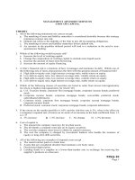
Eastman’s Cost of Equity Our first stop is the key statistics screen for Eastman
available at finance.yahoo.com (ticker: EMN). As of mid-2006, here’s what it looked
like:


According to this screen, Eastman has 81.8 million shares of stock outstanding. The
book value per share is $21.028, but the stock sells for $51.34. Total equity is therefore
about $1.72 billion on a book value basis, but it is closer to $4.20 billion on a market value
basis.

ros3062x_Ch15.indd 489

2/8/07 2:44:12 PM


490

PA RT 6

Cost of Capital and Long-Term Financial Policy

To estimate Eastman’s cost of equity, we will assume a market risk premium of
8.5 percent, similar to what we calculated in Chapter 12. Eastman’s beta on Yahoo! is 1.11,
which is only slightly higher than the beta of the average stock. To check this number, we
went to www.hoovers.com and www.msnbc.com. The beta estimates we found there were
0.90 and 0.94. These estimates of beta are lower than the estimate from Yahoo!, so we will
use an average of the three estimates, which is 0.983. According to the bond section of
finance.yahoo.com, T-bills were paying about 4.86 percent. Using the CAPM to estimate
the cost of equity, we find:
RE ϭ 0.0486 ϩ 0.983 (0.085) ϭ 0.1322 or 13.22%
Eastman has paid dividends for only a few years, so calculating the growth rate for the
dividend discount model is problematic. However, under the analysts’ estimates link at

ros3062x_Ch15.indd 490


2/8/07 2:44:12 PM


C H A P T E R 15 Cost of Capital

491

finance.yahoo.com, we found the following:

Analysts estimate the growth in earnings per share for the company will be 7 percent for
the next five years. For now, we will use this growth rate in the dividend discount model to
estimate the cost of equity; the link between earnings growth and dividends is discussed in
a later chapter. The estimated cost of equity using the dividend discount model is:
$1.76 (1 ϩ .07)
RE ϭ _____________ ϩ .07 ϭ .1069 or 10.69%
$51.34

[

]

Notice that the estimates for the cost of equity are different. This is often the
case. Remember that each method of estimating the cost of equity relies on different
assumptions, so different estimates of the cost of equity should not surprise us. If the
estimates are different, there are two simple solutions. First, we could ignore one of the
estimates. We would look at each estimate to see if one of them seemed too high or too
low to be reasonable. Second, we could average the two estimates. Averaging the two
estimates for Eastman’s cost of equity gives us a cost of equity of 11.94 percent. This
seems like a reasonable number, so we will use it in calculating the cost of capital in
this example.


Eastman’s Cost of Debt Eastman has six relatively long-term bond issues that account
for essentially all of its long-term debt. To calculate the cost of debt, we will have to combine these six issues. What we will do is compute a weighted average. We went to www.
nasdbondinfo.com to find quotes on the bonds. We should note here that finding the yield
to maturity for all of a company’s outstanding bond issues on a single day is unusual. If you
remember our previous discussion of bonds, the bond market is not as liquid as the stock
market; on many days, individual bond issues may not trade. To find the book value of the
bonds, we went to www.sec.gov and found the 10Q report dated March 31, 2006, and filed
with the SEC on May 3, 2006. The basic information is as follows:6
6

You might be wondering why the yield on the 7.625 percent issue maturing in 2024 is lower than that on the
other two long-term issues with similar maturities. The reason is that this issue has a put feature (discussed in
Chapter 7) that the other two issues do not. Such features are desirable from the buyer’s standpoint, so this issue
has a higher price and thus a lower yield.

ros3062x_Ch15.indd 491

2/8/07 2:44:13 PM


492

PA RT 6

Cost of Capital and Long-Term Financial Policy

Coupon
Rate
3.25%

7.00
6.30
7.25
7.625
7.60

Maturity

Book Value
(Face value,
in Millions)

Price
(% of Par)

Yield to
Maturity

2008
2012
2018
2024
2024
2027

$ 72
138
179
497
200

298

94.15
105.52
99.15
102.10
106.31
106.12

5.85
5.87
6.40
7.04
7.00
7.03

To calculate the weighted average cost of debt, we take the percentage of the total debt
represented by each issue and multiply by the yield on the issue. We then add to get the
overall weighted average debt cost. We use both book values and market values here for
comparison. The results of the calculations are as follows:

Coupon
Rate
3.25%
7.00
6.30
7.60
7.625
7.60
Total


Book Value
(Face value,
in Millions)
$

72
138
179
497
200
298
$1,384

Percentage
of Total
0.05
0.10
0.13
0.36
0.14
0.22
1.00

Market
Value
(in Millions)
$

67.79

145.61
177.47
507.44
212.62
316.25
$1,427.18

Percentage
of Total

Yield to
Maturity

Book
Values

Market
Values

0.05
0.10
0.12
0.36
0.15
0.22
1.00

5.85%
5.87
6.40

7.04
7.00
7.03

0.30%
0.59
0.83
2.53
1.01
1.51
6.77%

0.28%
0.60
0.80
2.50
1.04
1.56
6.78%

As these calculations show, Eastman’s cost of debt is 6.77 percent on a book value basis
and 6.78 percent on a market value basis. Thus, for Eastman, whether market values or
book values are used makes no difference. The reason is simply that the market values and
book values are similar. This will often be the case and explains why companies frequently
use book values for debt in WACC calculations. Also, Eastman has no preferred stock, so
we don’t need to consider its cost.

Eastman’s WACC We now have the various pieces necessary to calculate Eastman’s WACC.
First, we need to calculate the capital structure weights. On a book value basis, Eastman’s
equity and debt are worth $1.720 billion and $1.384 billion, respectively. The total value is

$3.104 billion, so the equity and debt percentages are $1.720 billion͞3.104 billion ϭ .55 and
$1.384 billion͞3.104 billion ϭ .45. Assuming a tax rate of 35 percent, Eastman’s WACC is:
WACC ϭ .55 ϫ 11.94% ϩ .45 ϫ 6.77% ϫ (1 Ϫ .35)
ϭ 8.55%
Thus, using book value capital structure weights, we get about 8.55 percent for Eastman’s
WACC.
If we use market value weights, however, the WACC will be higher. To see why,
notice that on a market value basis, Eastman’s equity and debt are worth $4.200 billion
and $1.427 billion, respectively. The capital structure weights are therefore $4.200
billion͞5.627 billion ϭ .75 and $1.427 billion͞5.627 billion ϭ .25, so the equity percentage is much higher. With these weights, Eastman’s WACC is:
WACC ϭ .75 ϫ 11.94% ϩ .25 ϫ 6.78% ϫ (1 Ϫ .35)
ϭ 10%

ros3062x_Ch15.indd 492

2/8/07 2:44:13 PM


493

C H A P T E R 15 Cost of Capital

Thus, using market value weights, we get about 10 percent for Eastman’s WACC, which is
about 1.5 percent higher than the 8.55 percent WACC we got using book value weights.
As this example illustrates, using book values can lead to trouble, particularly if equity book
values are used. Going back to Chapter 3, recall that we discussed the market-to-book ratio
(the ratio of market value per share to book value per share). This ratio is usually substantially
bigger than 1. For Eastman, for example, verify that it’s about 2.4; so book values significantly
overstate the percentage of Eastman’s financing that comes from debt. In addition, if we were
computing a WACC for a company that did not have publicly traded stock, we would try to

come up with a suitable market-to-book ratio by looking at publicly traded companies, and we
would then use this ratio to adjust the book value of the company under consideration. As we
have seen, failure to do so can lead to significant underestimation of the WACC.
Our nearby Work the Web box explains more about the WACC and related topics.

WORK THE WEB
So how does our estimate of the WACC for Eastman Chemical compare to others? One place to find estimates
for WACC is www.valuepro.net. We went there and found the following information for Eastman:

As you can see, ValuePro estimates the WACC (Cost of Capital) for Eastman as 7.31 percent, which is lower
than our estimate of 10 percent. You can see why the estimates for WACC are different: Different inputs were
used in the computations. For example, ValuePro uses an equity risk premium of only 3 percent. Calculating
WACC requires the estimation of various inputs, and you must use your best judgment in these estimates.

ros3062x_Ch15.indd 493

2/8/07 2:44:16 PM


494

PA RT 6

Cost of Capital and Long-Term Financial Policy

SOLVING THE WAREHOUSE PROBLEM AND SIMILAR
CAPITAL BUDGETING PROBLEMS
Now we can use the WACC to solve the warehouse problem we posed at the beginning of
the chapter. However, before we rush to discount the cash flows at the WACC to estimate
NPV, we need to make sure we are doing the right thing.

Going back to first principles, we need to find an alternative in the financial markets
that is comparable to the warehouse renovation. To be comparable, an alternative must be
of the same level of risk as the warehouse project. Projects that have the same risk are said
to be in the same risk class.
The WACC for a firm reflects the risk and the target capital structure of the firm’s existing assets as a whole. As a result, strictly speaking, the firm’s WACC is the appropriate
discount rate only if the proposed investment is a replica of the firm’s existing operating
activities.
In broader terms, whether or not we can use the firm’s WACC to value the warehouse
project depends on whether the warehouse project is in the same risk class as the firm.
We will assume that this project is an integral part of the overall business of the firm. In
such cases, it is natural to think that the cost savings will be as risky as the general cash
flows of the firm, and the project will thus be in the same risk class as the overall firm.
More generally, projects like the warehouse renovation that are intimately related to the
firm’s existing operations are often viewed as being in the same risk class as the overall
firm.
We can now see what the president should do. Suppose the firm has a target debt–equity
ratio of 1͞3. From Chapter 3, we know that a debt–equity ratio of D͞E ϭ 1͞3 implies that
E͞V is .75 and D͞V is .25. The cost of debt is 10 percent, and the cost of equity is 20 percent. Assuming a 34 percent tax rate, the WACC will be:
WACC ϭ (E͞V) ϫ RE ϩ (D͞V) ϫ RD ϫ (1 Ϫ TC)
ϭ .75 ϫ 20% ϩ .25 ϫ 10% ϫ (1 Ϫ .34)
ϭ 16.65%
Recall that the warehouse project had a cost of $50 million and expected aftertax cash
flows (the cost savings) of $12 million per year for six years. The NPV (in millions) is
thus:
12
12
NPV ϭ Ϫ$50 ϩ ____________
ϩ . . . ϩ ___________
(1ϩWACC)6
(1 ϩ WACC)1

Because the cash flows are in the form of an ordinary annuity, we can calculate this NPV
using 16.65 percent (the WACC) as the discount rate as follows:
1 Ϫ [1͞(1 ϩ .1665)6]
NPV ϭ Ϫ$50 ϩ 12 ϫ __________________
.1665
ϭ Ϫ$50 ϩ 12 ϫ 3.6222
ϭ Ϫ$6.53
Should the firm take on the warehouse renovation? The project has a negative NPV
using the firm’s WACC. This means that the financial markets offer superior projects
in the same risk class (namely, the firm itself). The answer is clear: The project should
be rejected. For future reference, our discussion of the WACC is summarized in
Table 15.1.

ros3062x_Ch15.indd 494

2/8/07 2:44:18 PM


495

C H A P T E R 15 Cost of Capital

I.

The Cost of Equity, RE

TABLE 15.1

A. Dividend growth model approach (from Chapter 8):


Summary of Capital Cost
Calculations

RE ϭ D1րP0 ϩ g
where D1 is the expected dividend in one period, g is the dividend growth rate, and P0 is
the current stock price.
B. SML approach (from Chapter 13):
RE ϭ Rf ϩ ␤E ϫ (RM Ϫ Rf)
where Rf is the risk-free rate, RM is the expected return on the overall market, and ␤E is
the systematic risk of the equity.
II.

The Cost of Debt, RD
A. For a firm with publicly held debt, the cost of debt can be measured as the yield to
maturity on the outstanding debt. The coupon rate is irrelevant. Yield to maturity is
covered in Chapter 7.
B. If the firm has no publicly traded debt, then the cost of debt can be measured as the
yield to maturity on similarly rated bonds (bond ratings are discussed in Chapter 7).

III.

The Weighted Average Cost of Capital, WACC
A. The firm’s WACC is the overall required return on the firm as a whole. It is the
appropriate discount rate to use for cash flows similar in risk to those of the overall firm.
B. The WACC is calculated as:
WACC ϭ (EրV ) ϫ RE ϩ (DրV ) ϫ RD ϫ (1 Ϫ TC)
where TC is the corporate tax rate, E is the market value of the firm’s equity, D is the
market value of the firm’s debt, and V ϭ E ϩ D. Note that EրV is the percentage of the
firm’s financing (in market value terms) that is equity, and DրV is the percentage that
is debt.


Using the WACC

EXAMPLE 15.5

A firm is considering a project that will result in initial aftertax cash savings of $5 million at
the end of the first year. These savings will grow at the rate of 5 percent per year. The firm
has a debt–equity ratio of .5, a cost of equity of 29.2 percent, and a cost of debt of 10 percent. The cost-saving proposal is closely related to the firm’s core business, so it is viewed
as having the same risk as the overall firm. Should the firm take on the project?
Assuming a 34 percent tax rate, the firm should take on this project if it costs less than
$30 million. To see this, first note that the PV is:
$5 million
PV ϭ ____________
WACC Ϫ .05
This is an example of a growing perpetuity as discussed in Chapter 6. The WACC is:
WACC ϭ (EրV ) ϫ RE ϩ (DրV ) ϫ RD ϫ (1 Ϫ TC)
ϭ 2ր3 ϫ 29.2% ϩ 1ր3 ϫ 10% ϫ (1 Ϫ .34)
ϭ 21.67%
The PV is thus:
$5 million ϭ $30 million
PV ϭ ___________
.2167 Ϫ .05
The NPV will be positive only if the cost is less than $30 million.

ros3062x_Ch15.indd 495

2/8/07 2:44:19 PM


IN THEIR OWN WORDS . . .

Bennett Stewart on EVA
A firm’s weighted average cost of capital has important applications other than the discount rate in capital project evaluations. For instance, it is a key ingredient to measure a firm’s true economic profit, or what
I like to call EVA, standing for economic value added. Accounting rules dictate that the interest expense a
company incurs on its debt financing be deducted from its reported profit, but those same rules ironically
forbid deducting a charge for the shareholders’ funds a firm uses. In economic terms, equity capital is in
fact a very costly financing source, because shareholders bear the risk of being paid last, after all other
stakeholders and investors are paid first. But according to accountants, shareholders equity is free.
This egregious oversight has dire practical consequences. For one thing, it means that the profit figure
accountants certify to be correct is inherently at odds with the net present value decision rule. For instance,
it is a simple matter for management to inflate its reported earnings and earnings-per-share in ways that
actually harm the shareholders by investing capital in projects that earn less than the overall cost of capital
but more than the aftertax cost of borrowing money, which amounts to a trivial hurdle in most cases, a couple percentage points at most. In effect, EPS requires management to vault a mere three foot hurdle when to
satisfy shareholders managers must jump a ten foot hurdle that includes the cost of equity. A prime example
of the way accounting profit leads smart managers to do dumb things was Enron, where former top executives Ken Lay and Jeff Skilling boldly declared in the firm’s 2000 annual report that they were “laser-focused
on earnings per share,” and so they were. Bonuses were funded out of book profit, and project developers were paid for signing up new deals and not generating a decent return on investment. Consequently,
Enron’s EPS was on the rise while its true economic profit—its EVA—measured after deducting the full cost
of capital, was plummeting in the years leading up to the firm’s demise—the result of massive misallocations
of capital to ill-advised energy and new economy projects. The point is, EVA measures economic profit, the
profit that actually discounts to net present value, and the maximization of which is every company’s most
important financial goal; yet for all its popularity EPS is just an accounting contrivance that is wholly unrelated to the maximization of shareholder wealth or sending the right decision signals to management.
Starting in the early 1990s firms around the world—ranging from Coca-Cola, to Briggs & Stratton,
Herman Miller, and Eli Lilly in America, Siemens in Germany, Tata Consulting and the Godrej Group out
of India, Brahma Beer in Brazil, and many, many more—began to turn to EVA as a new and better way to
measure performance and set goals, make decisions and determine bonuses, and to communicate with
investors and to teach business and finance basics to managers and employees. Properly tailored and
implemented, EVA is a natural way to bring the cost of capital to life, and to turn everyone in a company
into a capital conscientious, owner-entrepreneur.
Bennett Stewart is a co-founder of Stern Stewart & Co. and also the CEO of EVA Dimensions, a firm providing EVA data, valuation modeling, and hedge fund
management. Stewart pioneered the practical development of EVA as chronicled in his book, The Quest for Value.


PERFORMANCE EVALUATION: ANOTHER USE OF THE WACC
Visit
www.sternstewart.com
for more about EVA.

Looking back at the Eastman Chemical example we used to open the chapter, we see another
use of the WACC: its use for performance evaluation. Probably the best-known approach in
this area is the economic value added (EVA) method developed by Stern Stewart and Co.
Companies such as AT&T, Coca-Cola, Quaker Oats, and Briggs and Stratton are among the
firms that have been using EVA as a means of evaluating corporate performance. Similar
approaches include market value added (MVA) and shareholder value added (SVA).
Although the details differ, the basic idea behind EVA and similar strategies is straightforward. Suppose we have $100 million in capital (debt and equity) tied up in our firm, and
our overall WACC is 12 percent. If we multiply these together, we get $12 million. Referring
back to Chapter 2, if our cash flow from assets is less than this, we are, on an overall basis,
destroying value; if cash flow from assets exceeds $12 million, we are creating value.
In practice, evaluation strategies such as these suffer to a certain extent from problems
with implementation. For example, it appears that Eastman Chemical and others make

496

ros3062x_Ch15.indd 496

2/8/07 2:44:20 PM


497

C H A P T E R 15 Cost of Capital

extensive use of book values for debt and equity in computing cost of capital. Even so,

by focusing on value creation, WACC-based evaluation procedures force employees and
management to pay attention to the real bottom line: increasing share prices.

Concept Questions
15.4a How is the WACC calculated?
15.4b Why do we multiply the cost of debt by (1 Ϫ TC) when we compute the WACC?
15.4c Under what conditions is it correct to use the WACC to determine NPV?

Divisional and
Project Costs of Capital

15.5

As we have seen, using the WACC as the discount rate for future cash flows is appropriate
only when the proposed investment is similar to the firm’s existing activities. This is not
as restrictive as it sounds. If we are in the pizza business, for example, and we are thinking
of opening a new location, then the WACC is the discount rate to use. The same is true of
a retailer thinking of a new store, a manufacturer thinking of expanding production, or a
consumer products company thinking of expanding its markets.
Nonetheless, despite the usefulness of the WACC as a benchmark, there will clearly be
situations in which the cash flows under consideration have risks distinctly different from
those of the overall firm. We consider how to cope with this problem next.

THE SML AND THE WACC
When we are evaluating investments with risks that are substantially different from those
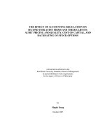
of the overall firm, use of the WACC will potentially lead to poor decisions. Figure 15.1
illustrates why.
In Figure 15.1, we have plotted an SML corresponding to a risk-free rate of 7 percent
and a market risk premium of 8 percent. To keep things simple, we consider an all-equity
company with a beta of 1. As we have indicated, the WACC and the cost of equity are

exactly equal to 15 percent for this company because there is no debt.
Suppose our firm uses its WACC to evaluate all investments. This means that any
investment with a return of greater than 15 percent will be accepted and any investment
with a return of less than 15 percent will be rejected. We know from our study of risk and
return, however, that a desirable investment is one that plots above the SML. As Figure 15.1
illustrates, using the WACC for all types of projects can result in the firm’s incorrectly
accepting relatively risky projects and incorrectly rejecting relatively safe ones.
For example, consider point A. This project has a beta of ␤A ϭ .60, as compared to the
firm’s beta of 1.0. It has an expected return of 14 percent. Is this a desirable investment?
The answer is yes because its required return is only:
Required return ϭ Rf ϩ ␤A ϫ (RM Ϫ Rf)
ϭ 7% ϩ .60 ϫ 8%
ϭ 11.8%
However, if we use the WACC as a cutoff, then this project will be rejected because its
return is less than 15 percent. This example illustrates that a firm that uses its WACC as a
cutoff will tend to reject profitable projects with risks less than those of the overall firm.

ros3062x_Ch15.indd 497

2/8/07 2:44:22 PM


498

PA RT 6

Cost of Capital and Long-Term Financial Policy

FIGURE 15.1
The Security Market

Line (SML) and the
Weighted Average Cost
of Capital (WACC)

SML

Expected return (%)

ϭ 8%
B

16
15
14

A

Incorrect
acceptance
WACC ϭ 15%

Incorrect
rejection

Rf ϭ 7

␤A ϭ .60

␤firm ϭ 1.0 ␤B ϭ 1.2
Beta


If a firm uses its WACC to make accept–reject decisions for all types of projects, it will have
a tendency toward incorrectly accepting risky projects and incorrectly rejecting less risky
projects.

At the other extreme, consider point B. This project has a beta of ␤B ϭ 1.2. It offers a
16 percent return, which exceeds the firm’s cost of capital. This is not a good investment,
however, because, given its level of systematic risk, its return is inadequate. Nonetheless, if
we use the WACC to evaluate it, it will appear to be attractive. So the second error that will
arise if we use the WACC as a cutoff is that we will tend to make unprofitable investments
with risks greater than those of the overall firm. As a consequence, through time, a firm
that uses its WACC to evaluate all projects will have a tendency to both accept unprofitable
investments and become increasingly risky.

DIVISIONAL COST OF CAPITAL
The same type of problem with the WACC can arise in a corporation with more than one
line of business. Imagine, for example, a corporation that has two divisions: a regulated
telephone company and an electronics manufacturing operation. The first of these (the
phone operation) has relatively low risk; the second has relatively high risk.
In this case, the firm’s overall cost of capital is really a mixture of two different costs
of capital, one for each division. If the two divisions were competing for resources, and
the firm used a single WACC as a cutoff, which division would tend to be awarded greater
funds for investment?
The answer is that the riskier division would tend to have greater returns (ignoring the
greater risk), so it would tend to be the “winner.” The less glamorous operation might have
great profit potential that would end up being ignored. Large corporations in the United States
are aware of this problem, and many work to develop separate divisional costs of capital.

THE PURE PLAY APPROACH
We’ve seen that using the firm’s WACC inappropriately can lead to problems. How can

we come up with the appropriate discount rates in such circumstances? Because we cannot
observe the returns on these investments, there generally is no direct way of coming up

ros3062x_Ch15.indd 498

2/8/07 2:44:24 PM


499

C H A P T E R 15 Cost of Capital

with a beta, for example. Instead, what we must do is examine other investments outside
the firm that are in the same risk class as the one we are considering, and use the marketrequired return on these investments as the discount rate. In other words, we will try to
determine what the cost of capital is for such investments by trying to locate some similar
investments in the marketplace.
For example, going back to our telephone division, suppose we wanted to come up with
a discount rate to use for that division. What we could do is identify several other phone
companies that have publicly traded securities. We might find that a typical phone company has a beta of .80, AA-rated debt, and a capital structure that is about 50 percent debt
and 50 percent equity. Using this information, we could develop a WACC for a typical
phone company and use this as our discount rate.
Alternatively, if we were thinking of entering a new line of business, we would try to
develop the appropriate cost of capital by looking at the market-required returns on companies already in that business. In the language of Wall Street, a company that focuses on a
single line of business is called a pure play. For example, if you wanted to bet on the price
of crude oil by purchasing common stocks, you would try to identify companies that dealt
exclusively with this product because they would be the most affected by changes in the
price of crude oil. Such companies would be called “pure plays on the price of crude oil.”
What we try to do here is to find companies that focus as exclusively as possible on
the type of project in which we are interested. Our approach, therefore, is called the pure
play approach to estimating the required return on an investment. To illustrate, suppose

McDonald’s decides to enter the personal computer and network server business with a
line of machines called McPuters. The risks involved are quite different from those in the
fast-food business. As a result, McDonald’s would need to look at companies already in the
personal computer business to compute a cost of capital for the new division. Two obvious
pure play candidates would be Dell and Gateway, which are predominantly in this line of
business. IBM, on the other hand, would not be as good a choice because its primary focus
is elsewhere, and it has many different product lines.
In Chapter 3, we discussed the subject of identifying similar companies for comparison
purposes. The same problems we described there come up here. The most obvious one is
that we may not be able to find any suitable companies. In this case, how to objectively
determine a discount rate becomes a difficult question. Even so, the important thing is to
be aware of the issue so that we at least reduce the possibility of the kinds of mistakes that
can arise when the WACC is used as a cutoff on all investments.

pure play approach
The use of a WACC that
is unique to a particular
project, based on
companies in similar lines
of business.

THE SUBJECTIVE APPROACH
Because of the difficulties that exist in objectively establishing discount rates for individual projects, firms often adopt an approach that involves making subjective adjustments
to the overall WACC. To illustrate, suppose a firm has an overall WACC of 14 percent.
It places all proposed projects into four categories as follows:
Category
High risk
Moderate risk
Low risk
Mandatory


Examples
New products
Cost savings, expansion of
existing lines
Replacement of existing
equipment
Pollution control equipment

Adjustment Factor

Discount Rate

ϩ6%

20%

ϩ0

14

Ϫ4
n/a

10
n/a

n͞a ϭ Not applicable.

ros3062x_Ch15.indd 499


2/8/07 2:44:24 PM


500

PA RT 6

Cost of Capital and Long-Term Financial Policy

FIGURE 15.2 The Security Market Line (SML) and the Subjective Approach

SML
ϭ 8%
Expected return (%)

20

A

High risk
(ϩ6%)

WACC ϭ 14
10
Rf ϭ 7
Low risk
(Ϫ4%)

Moderate risk

(ϩ0%)

Beta
With the subjective approach, the firm places projects into one of several risk classes. The
discount rate used to value the project is then determined by adding (for high risk) or
subtracting (for low risk) an adjustment factor to or from the firm’s WACC. This results in
fewer incorrect decisions than if the firm simply used the WACC to make the decisions.

The effect of this crude partitioning is to assume that all projects either fall into one of three
risk classes or else are mandatory. In the last case, the cost of capital is irrelevant because the
project must be taken. With the subjective approach, the firm’s WACC may change through
time as economic conditions change. As this happens, the discount rates for the different
types of projects will also change.
Within each risk class, some projects will presumably have more risk than others, and
the danger of making incorrect decisions still exists. Figure 15.2 illustrates this point. Comparing Figures 15.1 and 15.2, we see that similar problems exist; but the magnitude of the
potential error is less with the subjective approach. For example, the project labeled A
would be accepted if the WACC were used, but it is rejected once it is classified as a highrisk investment. What this illustrates is that some risk adjustment, even if it is subjective,
is probably better than no risk adjustment.
It would be better, in principle, to objectively determine the required return for each
project separately. However, as a practical matter, it may not be possible to go much
beyond subjective adjustments because either the necessary information is unavailable or
the cost and effort required are simply not worthwhile.

Concept Questions
15.5a What are the likely consequences if a firm uses its WACC to evaluate all proposed investments?
15.5b What is the pure play approach to determining the appropriate discount rate?
When might it be used?

ros3062x_Ch15.indd 500


2/8/07 2:44:25 PM


501

C H A P T E R 15 Cost of Capital

Flotation Costs and the Weighted
Average Cost of Capital

15.6

So far, we have not included issue, or flotation, costs in our discussion of the weighted
average cost of capital. If a company accepts a new project, it may be required to issue, or
float, new bonds and stocks. This means that the firm will incur some costs, which we call
flotation costs. The nature and magnitude of flotation costs are discussed in some detail in
Chapter 16.
Sometimes it is suggested that the firm’s WACC should be adjusted upward to reflect
flotation costs. This is really not the best approach because, once again, the required return
on an investment depends on the risk of the investment, not the source of the funds. This is
not to say that flotation costs should be ignored. Because these costs arise as a consequence
of the decision to undertake a project, they are relevant cash flows. We therefore briefly
discuss how to include them in project analysis.

THE BASIC APPROACH
We start with a simple case. The Spatt Company, an all-equity firm, has a cost of equity
of 20 percent. Because this firm is 100 percent equity, its WACC and its cost of equity are
the same. Spatt is contemplating a large-scale $100 million expansion of its existing operations. The expansion would be funded by selling new stock.
Based on conversations with its investment banker, Spatt believes its flotation costs will
run 10 percent of the amount issued. This means that Spatt’s proceeds from the equity sale

will be only 90 percent of the amount sold. When flotation costs are considered, what is the
cost of the expansion?
As we discuss in more detail in Chapter 16, Spatt needs to sell enough equity to raise
$100 million after covering the flotation costs. In other words:
$100 million ϭ (1 Ϫ .10) ϫ Amount raised
Amount raised ϭ $100 million͞.90 ϭ $111.11 million
Spatt’s flotation costs are thus $11.11 million, and the true cost of the expansion is
$111.11 million once we include flotation costs.
Things are only slightly more complicated if the firm uses both debt and equity. For
example, suppose Spatt’s target capital structure is 60 percent equity, 40 percent debt. The
flotation costs associated with equity are still 10 percent, but the flotation costs for debt are
less—say 5 percent.
Earlier, when we had different capital costs for debt and equity, we calculated a weighted
average cost of capital using the target capital structure weights. Here we will do much the
same thing. We can calculate a weighted average flotation cost, fA, by multiplying the
equity flotation cost, fE, by the percentage of equity (E͞V) and the debt flotation cost, fD, by
the percentage of debt (D͞V) and then adding the two together:
fA ϭ (E͞V ) ϫ fE ϩ (D͞V ) ϫ fD
[15.8]
ϭ 60% ϫ .10 ϩ 40% ϫ .05
ϭ 8%
The weighted average flotation cost is thus 8 percent. What this tells us is that for every
dollar in outside financing needed for new projects, the firm must actually raise $1͞(1 Ϫ
.08) ϭ $1.087. In our example, the project cost is $100 million when we ignore flotation
costs. If we include them, then the true cost is $100 million͞(1 Ϫ fA) ϭ $100 million͞.92 ϭ
$108.7 million.

ros3062x_Ch15.indd 501

2/8/07 2:44:25 PM



502

PA RT 6

Cost of Capital and Long-Term Financial Policy

In taking issue costs into account, the firm must be careful not to use the wrong weights.
The firm should use the target weights, even if it can finance the entire cost of the project
with either debt or equity. The fact that a firm can finance a specific project with debt or
equity is not directly relevant. If a firm has a target debt–equity ratio of 1, for example, but
chooses to finance a particular project with all debt, it will have to raise additional equity
later on to maintain its target debt–equity ratio. To take this into account, the firm should
always use the target weights in calculating the flotation cost.

EXAMPLE 15.6

Calculating the Weighted Average Flotation Cost
The Weinstein Corporation has a target capital structure that is 80 percent equity, 20 percent
debt. The flotation costs for equity issues are 20 percent of the amount raised; the flotation
costs for debt issues are 6 percent. If Weinstein needs $65 million for a new manufacturing
facility, what is the true cost once flotation costs are considered?
We first calculate the weighted average flotation cost, fA:
fA ϭ (E͞V ) ϫ fE ϩ (D͞V ) ϫ fD
ϭ 80% ϫ .20 ϩ 20% ϫ .06
ϭ 17.2%
The weighted average flotation cost is thus 17.2 percent. The project cost is $65 million when
we ignore flotation costs. If we include them, then the true cost is $65 million͞(1 Ϫ fA) ϭ $65
million͞.828 ϭ $78.5 million, again illustrating that flotation costs can be a considerable

expense.

FLOTATION COSTS AND NPV
To illustrate how flotation costs can be included in an NPV analysis, suppose the Tripleday
Printing Company is currently at its target debt–equity ratio of 100 percent. It is considering building a new $500,000 printing plant in Kansas. This new plant is expected to generate aftertax cash flows of $73,150 per year forever. The tax rate is 34 percent. There are
two financing options:
1. A $500,000 new issue of common stock: The issuance costs of the new common stock
would be about 10 percent of the amount raised. The required return on the company’s
new equity is 20 percent.
2. A $500,000 issue of 30-year bonds: The issuance costs of the new debt would be
2 percent of the proceeds. The company can raise new debt at 10 percent.
What is the NPV of the new printing plant?
To begin, because printing is the company’s main line of business, we will use the
company’s weighted average cost of capital to value the new printing plant:
WACC ϭ (E͞V) ϫ RE ϩ (D͞V) ϫ RD ϫ (1 Ϫ TC)
ϭ .50 ϫ 20% ϩ .50 ϫ 10% ϫ (1 Ϫ .34)
ϭ 13.3%
Because the cash flows are $73,150 per year forever, the PV of the cash flows at 13.3 percent
per year is:
$73,150 ϭ $550,000
PV ϭ _______
.133

ros3062x_Ch15.indd 502

2/8/07 2:44:26 PM


IN THEIR OWN WORDS . . .
Samuel Weaver on Cost of Capital and Hurdle Rates at The Hershey Company

At Hershey, we reevaluate our cost of capital annually or as market conditions warrant. The calculation of
the cost of capital essentially involves three different issues, each with a few alternatives:
• Capital structure weighting
Historical book value
Target capital structure
Market-based weights
• Cost of debt
Historical (coupon) interest rates
Market-based interest rates
• Cost of equity
Dividend growth model
Capital asset pricing model, or CAPM
At Hershey, we calculate our cost of capital officially based on the projected “target” capital structure at
the end of our three-year intermediate planning horizon. This allows management to see the immediate
impact of strategic decisions related to the planned composition of Hershey’s capital pool. The cost of debt
is calculated as the anticipated weighted average aftertax cost of debt in that final plan year based on the
coupon rates attached to that debt. The cost of equity is computed via the dividend growth model.
We recently conducted a survey of the 11 food processing companies that we consider our industry group
competitors. The results of this survey indicated that the cost of capital for most of these companies was in
the 10 to 12 percent range. Furthermore, without exception, all 11 of these companies employed the CAPM
when calculating their cost of equity. Our experience has been that the dividend growth model works better
for Hershey. We do pay dividends, and we do experience steady, stable growth in our dividends. This growth
is also projected within our strategic plan. Consequently, the dividend growth model is technically applicable
and appealing to management because it reflects their best estimate of the future long-term growth rate.
In addition to the calculation already described, the other possible combinations and permutations are
calculated as barometers. Unofficially, the cost of capital is calculated using market weights, current marginal
interest rates, and the CAPM cost of equity. For the most part, and due to rounding the cost of capital to the
nearest whole percentage point, these alternative calculations yield approximately the same results.
From the cost of capital, individual project hurdle rates are developed using a subjectively determined risk
premium based on the characteristics of the project. Projects are grouped into separate project categories,

such as cost savings, capacity expansion, product line extension, and new products. For example, in general, a new product is more risky than a cost savings project. Consequently, each project category’s hurdle
rate reflects the level of risk and commensurate required return as perceived by senior management. As a
result, capital project hurdle rates range from a slight premium over the cost of capital to the highest hurdle
rate of approximately double the cost of capital.
Samuel Weaver, Ph.D., was formerly director, financial planning and analysis, for Hershey Chocolate North America. He is a certified management accountant and certified
financial manager. His position combined the theoretical with the pragmatic and involved the analysis of many different facets of finance in addition to capital expenditure analysis.

If we ignore flotation costs, the NPV is:
NPV ϭ $550,000 Ϫ 500,000 ϭ $50,000
With no flotation costs, the project generates an NPV that is greater than zero, so it should
be accepted.
What about financing arrangements and issue costs? Because new financing must be
raised, the flotation costs are relevant. From the information given, we know that the flotation costs are 2 percent for debt and 10 percent for equity. Because Tripleday uses equal
amounts of debt and equity, the weighted average flotation cost, fA, is:
fA ϭ (E͞V) ϫ fE ϩ (D͞V) ϫ fD ϭ .50 ϫ 10% ϩ .50 ϫ 2%
ϭ 6%
503

ros3062x_Ch15.indd 503

2/8/07 2:44:28 PM