Chapter 13 return, risk, and the security market line
Bạn đang xem bản rút gọn của tài liệu. Xem và tải ngay bản đầy đủ của tài liệu tại đây (2.15 MB, 36 trang )
On July 20, 2006, Apple Computer, Honeywell, and
The news for all three of these companies seemed
Yum Brands joined a host of other companies in
positive, but one stock rose on the news and the other
announcing earnings. All three companies announced
two stocks fell. So when is good news really good
earnings increases, ranging from 8 percent for Yum
news? The answer is fundamental to understanding
Brands to 48 percent for Apple. You would expect an
risk and return, and—the good news is—this chapter
earnings increase to be good news, and it is usually
explores it in some detail.
is. Apple’s stock jumped 12 percent on the news;
but unfortunately for Honeywell and Yum Brands,
their stock prices fell by 4.2 percent and 6.4 percent,
respectively.
Visit us at www.mhhe.com/rwj
DIGITAL STUDY TOOLS
• Self-Study Software
• Multiple-Choice Quizzes
• Flashcards for Testing and
Key Terms
In our last chapter, we learned some important lessons from capital market history. Most important, we learned that there is a reward, on average,
for bearing risk. We called this reward a risk premium. The second lesson is that this risk
premium is larger for riskier investments. This chapter explores the economic and managerial implications of this basic idea.
Thus far, we have concentrated mainly on the return behavior of a few large portfolios.
We need to expand our consideration to include individual assets. Specifically, we have
two tasks to accomplish. First, we have to define risk and discuss how to measure it. We
then must quantify the relationship between an asset’s risk and its required return.
When we examine the risks associated with individual assets, we find there are two types
of risk: systematic and unsystematic. This distinction is crucial because, as we will see,
systematic risk affects almost all assets in the economy, at least to some degree, whereas
unsystematic risk affects at most a small number of assets. We then develop the principle
of diversification, which shows that highly diversified portfolios will tend to have almost
no unsystematic risk.
The principle of diversification has an important implication: To a diversified investor,
only systematic risk matters. It follows that in deciding whether to buy a particular individual asset, a diversified investor will only be concerned with that asset’s systematic risk.
This is a key observation, and it allows us to say a great deal about the risks and returns
on individual assets. In particular, it is the basis for a famous relationship between risk
and return called the security market line, or SML. To develop the SML, we introduce the
equally famous “beta” coefficient, one of the centerpieces of modern finance. Beta and the
SML are key concepts because they supply us with at least part of the answer to the question of how to determine the required return on an investment.
Capital
Risk and
Budgeting
Return P A R T 45
13
RETURN, RISK, AND THE
SECURITY MARKET LINE
403
ros3062x_Ch13.indd 403
2/23/07 11:00:33 AM
404
PA RT 5
Risk and Return
13.1 Expected Returns and Variances
In our previous chapter, we discussed how to calculate average returns and variances using
historical data. We now begin to discuss how to analyze returns and variances when the
information we have concerns future possible returns and their probabilities.
EXPECTED RETURN
expected return
The return on a risky asset
expected in the future.
We start with a straightforward case. Consider a single period of time—say a year. We
have two stocks, L and U, which have the following characteristics: Stock L is expected
to have a return of 25 percent in the coming year. Stock U is expected to have a return of
20 percent for the same period.
In a situation like this, if all investors agreed on the expected returns, why would anyone want to hold Stock U? After all, why invest in one stock when the expectation is that
another will do better? Clearly, the answer must depend on the risk of the two investments.
The return on Stock L, although it is expected to be 25 percent, could actually turn out to
be higher or lower.
For example, suppose the economy booms. In this case, we think Stock L will have a
70 percent return. If the economy enters a recession, we think the return will be Ϫ20 percent.
In this case, we say that there are two states of the economy, which means that these are
the only two possible situations. This setup is oversimplified, of course, but it allows us to
illustrate some key ideas without a lot of computation.
Suppose we think a boom and a recession are equally likely to happen, for a 50–50
chance of each. Table 13.1 illustrates the basic information we have described and some
additional information about Stock U. Notice that Stock U earns 30 percent if there is a
recession and 10 percent if there is a boom.
Obviously, if you buy one of these stocks, say Stock U, what you earn in any particular
year depends on what the economy does during that year. However, suppose the probabilities stay the same through time. If you hold Stock U for a number of years, you’ll earn
30 percent about half the time and 10 percent the other half. In this case, we say that your
expected return on Stock U, E(RU ), is 20 percent:
E(RU ) ϭ .50 ϫ 30% ϩ .50 ϫ 10% ϭ 20%
In other words, you should expect to earn 20 percent from this stock, on average.
For Stock L, the probabilities are the same, but the possible returns are different. Here,
we lose 20 percent half the time, and we gain 70 percent the other half. The expected return
on L, E(RL ), is thus 25 percent:
E(RL ) ϭ .50 ϫ Ϫ20% ϩ .50 ϫ 70% ϭ 25%
Table 13.2 illustrates these calculations.
In our previous chapter, we defined the risk premium as the difference between the
return on a risky investment and that on a risk-free investment, and we calculated the
historical risk premiums on some different investments. Using our projected returns,
TABLE 13.1
States of the Economy
and Stock Returns
ros3062x_Ch13.indd 404
State of
Economy
Probability of
State of Economy
Recession
Boom
.50
.50
1.00
Rate of Return if State Occurs
Stock L
Stock U
Ϫ20%
70
30%
10
2/8/07 2:37:29 PM
C H A P T E R 13
Stock L
(1)
State of
Economy
Recession
Boom
(2)
Probability
of State of
Economy
.50
.50
1.00
(3)
Rate of
Return
if State
Occurs
405
Return, Risk, and the Security Market Line
(4)
Product
(2) ϫ (3)
Ϫ.20
Ϫ.10
.70
.35
E(RL ) ϭ .25 ϭ 25%
TABLE 13.2
Stock U
Calculation of Expected
Return
(5)
Rate of
Return
if State
Occurs
(6)
Product
(2) ϫ (5)
.30
.10
.15
.05
E(RU ) ϭ .20 ϭ 20%
we can calculate the projected, or expected, risk premium as the difference between the
expected return on a risky investment and the certain return on a risk-free investment.
For example, suppose risk-free investments are currently offering 8 percent. We will
say that the risk-free rate, which we label as Rf , is 8 percent. Given this, what is the projected risk premium on Stock U? On Stock L? Because the expected return on Stock U,
E(RU ), is 20 percent, the projected risk premium is:
Risk premium ϭ Expected return Ϫ Risk-free rate
ϭ E(RU ) Ϫ Rf
ϭ 20% Ϫ 8%
ϭ 12%
[13.1]
Similarly, the risk premium on Stock L is 25% Ϫ 8% ϭ 17%.
In general, the expected return on a security or other asset is simply equal to the sum
of the possible returns multiplied by their probabilities. So, if we had 100 possible returns,
we would multiply each one by its probability and add up the results. The result would be
the expected return. The risk premium would then be the difference between this expected
return and the risk-free rate.
Unequal Probabilities
EXAMPLE 13.1
Look again at Tables 13.1 and 13.2. Suppose you think a boom will occur only 20 percent
of the time instead of 50 percent. What are the expected returns on Stocks U and L in this
case? If the risk-free rate is 10 percent, what are the risk premiums?
The first thing to notice is that a recession must occur 80 percent of the time (1 Ϫ .20 ϭ
.80) because there are only two possibilities. With this in mind, we see that Stock U has a
30 percent return in 80 percent of the years and a 10 percent return in 20 percent of the
years. To calculate the expected return, we again just multiply the possibilities by the probabilities and add up the results:
E(RU ) ϭ .80 ϫ 30% ϩ .20 ϫ 10% ϭ 26%
Table 13.3 summarizes the calculations for both stocks. Notice that the expected return
on L is Ϫ2 percent.
The risk premium for Stock U is 26% Ϫ 10% ϭ 16% in this case. The risk premium for
Stock L is negative: Ϫ2% Ϫ 10% ϭ Ϫ12%. This is a little odd; but, for reasons we discuss
later, it is not impossible.
(continued)
ros3062x_Ch13.indd 405
2/8/07 2:37:30 PM
406
PA RT 5
Risk and Return
TABLE 13.3
Stock L
Calculation of Expected
Return
(1)
State of
Economy
(2)
Probability
of State of
Economy
(3)
Rate of
Return
if State
Occurs
Recession
Boom
.80
.20
Ϫ.20
.70
(4)
Product
(2) ؋ (3)
Ϫ.16
.14
E(RL) ϭ Ϫ2%
Stock U
(5)
Rate of
Return
if State
Occurs
.30
.10
(6)
Product
(2) ؋ (5)
.24
.02
E(RU) ϭ 26%
CALCULATING THE VARIANCE
To calculate the variances of the returns on our two stocks, we first determine the squared
deviations from the expected return. We then multiply each possible squared deviation by
its probability. We add these up, and the result is the variance. The standard deviation, as
always, is the square root of the variance.
To illustrate, let us return to the Stock U we originally discussed, which has an expected
return of E(RU ) ϭ 20%. In a given year, it will actually return either 30 percent or 10 percent.
The possible deviations are thus 30% Ϫ 20% ϭ 10% and 10% Ϫ 20% ϭ Ϫ10%. In this
case, the variance is:
Variance ϭ 2 ϭ .50 ϫ (10%)2 ϩ .50 ϫ(Ϫ10%)2 ϭ .01
The standard deviation is the square root of this:
Standard deviation ϭ ϭ ͙හහ
.01 ϭ .10 ϭ 10%
Table 13.4 summarizes these calculations for both stocks. Notice that Stock L has a much
larger variance.
When we put the expected return and variability information for our two stocks together,
we have the following:
Expected return, E(R)
Variance, 2
Standard deviation,
Stock L
Stock U
25%
.2025
45%
20%
.0100
10%
Stock L has a higher expected return, but U has less risk. You could get a 70 percent return
on your investment in L, but you could also lose 20 percent. Notice that an investment in
U will always pay at least 10 percent.
Which of these two stocks should you buy? We can’t really say; it depends on your
personal preferences. We can be reasonably sure that some investors would prefer L to U
and some would prefer U to L.
You’ve probably noticed that the way we have calculated expected returns and variances here is somewhat different from the way we did it in the last chapter. The reason
is that in Chapter 12, we were examining actual historical returns, so we estimated the
average return and the variance based on some actual events. Here, we have projected
future returns and their associated probabilities, so this is the information with which we
must work.
ros3062x_Ch13.indd 406
2/9/07 6:37:39 PM
C H A P T E R 13
407
Return, Risk, and the Security Market Line
(1)
State of
Economy
(2)
Probability
of State of
Economy
(3)
Return Deviation
from Expected
Return
(4)
Squared Return
Deviation from
Expected Return
Stock L
Recession
Boom
.50
.50
Ϫ.20 Ϫ .25 ϭ Ϫ.45
.70 Ϫ .25 ϭ .45
Ϫ.452 ϭ .2025
.452 ϭ .2025
TABLE 13.4
(5)
Product
(2) ؋ (4)
Calculation of Variance
.10125
.10125
2L ϭ .20250
Stock U
Recession
Boom
.50
.50
.30 Ϫ .20 ϭ .10
.10 Ϫ .20 ϭ Ϫ.10
.102 ϭ .01
Ϫ.102 ϭ .01
.005
.005
2U ϭ .010
More Unequal Probabilities
EXAMPLE 13.2
Going back to Example 13.1, what are the variances on the two stocks once we have
unequal probabilities? The standard deviations?
We can summarize the needed calculations as follows:
(1)
State of
Economy
(2)
Probability
of State of
Economy
(3)
Return Deviation
from Expected
Return
(4)
Squared Return
Deviation from
Expected Return
(5)
Product
(2) ؋ (4)
Stock L
Recession
Boom
.80
.20
Ϫ.20 Ϫ (Ϫ.02) ϭ Ϫ.18
.70 Ϫ (Ϫ.02) ϭ .72
.0324
.5184
.02592
.10368
2L ϭ .12960
Stock U
Recession
Boom
.80
.20
.30 Ϫ .26 ϭ .04
.10 Ϫ .26 ϭ Ϫ.16
.0016
.0256
.00128
.00512
2U ϭ .00640
Based on these calculations, the standard deviation for L is L ϭ ͙හහහ
.1296 ϭ .36 ϭ 36%.
The standard deviation for U is much smaller: U ϭ ͙හහහ
.0064 ϭ .08 or 8%.
Concept Questions
13.1a How do we calculate the expected return on a security?
13.1b In words, how do we calculate the variance of the expected return?
Portfolios
13.2
Thus far in this chapter, we have concentrated on individual assets considered separately.
However, most investors actually hold a portfolio of assets. All we mean by this is that
investors tend to own more than just a single stock, bond, or other asset. Given that this
is so, portfolio return and portfolio risk are of obvious relevance. Accordingly, we now
discuss portfolio expected returns and variances.
ros3062x_Ch13.indd 407
2/9/07 6:37:42 PM
408
PA RT 5
Risk and Return
TABLE 13.5
Expected Return on
an Equally Weighted
Portfolio of Stock L and
Stock U
(1)
State of
Economy
(2)
Probability
of State of
Economy
Recession
Boom
.50
.50
(3)
Portfolio Return if State Occurs
(4)
Product
(2) ؋ (3)
.50 ϫ Ϫ 20% ϩ .50 ϫ 30% ϭ 5%
.025
.50 ϫ
70% ϩ .50 ϫ 10% ϭ 40%
.200
E(RP) ϭ 22.5%
PORTFOLIO WEIGHTS
portfolio
A group of assets such as
stocks and bonds held by
an investor.
There are many equivalent ways of describing a portfolio. The most convenient approach
is to list the percentage of the total portfolio’s value that is invested in each portfolio asset.
We call these percentages the portfolio weights.
For example, if we have $50 in one asset and $150 in another, our total portfolio is
worth $200. The percentage of our portfolio in the first asset is $50͞$200 ϭ .25. The percentage of our portfolio in the second asset is $150͞$200, or .75. Our portfolio weights are
thus .25 and .75. Notice that the weights have to add up to 1.00 because all of our money
is invested somewhere.1
PORTFOLIO EXPECTED RETURNS
portfolio weight
The percentage of a
portfolio’s total value that
is in a particular asset.
Let’s go back to Stocks L and U. You put half your money in each. The portfolio weights are
obviously .50 and .50. What is the pattern of returns on this portfolio? The expected return?
To answer these questions, suppose the economy actually enters a recession. In this
case, half your money (the half in L) loses 20 percent. The other half (the half in U) gains
30 percent. Your portfolio return, RP, in a recession is thus:
RP ϭ .50 ϫ Ϫ20% ϩ .50 ϫ 30% ϭ 5%
Table 13.5 summarizes the remaining calculations. Notice that when a boom occurs, your
portfolio will return 40 percent:
RP ϭ .50 ϫ 70% ϩ .50 ϫ 10% ϭ 40%
As indicated in Table 13.5, the expected return on your portfolio, E(RP ), is 22.5 percent.
We can save ourselves some work by calculating the expected return more directly.
Given these portfolio weights, we could have reasoned that we expect half of our money
to earn 25 percent (the half in L) and half of our money to earn 20 percent (the half in U).
Our portfolio expected return is thus:
Want more
information about
investing? Take a look
at TheStreet.com’s
investing basics at
www.thestreet.com/basics.
E(RP ) ϭ .50 ϫ E(RL ) ϩ .50 ϫ E(RU )
ϭ .50 ϫ 25% ϩ .50 ϫ 20%
ϭ 22.5%
This is the same portfolio expected return we calculated previously.
This method of calculating the expected return on a portfolio works no matter how
many assets there are in the portfolio. Suppose we had n assets in our portfolio, where n is
any number. If we let xi stand for the percentage of our money in Asset i, then the expected
return would be:
[13.2]
E(R ) ϭ x ϫ E(R ) ϩ x ϫ E(R ) ϩ . . . ϩ x ϫ E(R )
P
1
1
2
2
n
n
1
Some of it could be in cash, of course, but we would then just consider the cash to be one of the portfolio
assets.
ros3062x_Ch13.indd 408
2/8/07 2:37:33 PM
C H A P T E R 13
Return, Risk, and the Security Market Line
409
This says that the expected return on a portfolio is a straightforward combination of the
expected returns on the assets in that portfolio. This seems somewhat obvious; but, as we
will examine next, the obvious approach is not always the right one.
Portfolio Expected Return
EXAMPLE 13.3
Suppose we have the following projections for three stocks:
State of
Economy
Probability of
State of Economy
Boom
Bust
.40
.60
Returns if State Occurs
Stock A
Stock B
10%
8
15%
4
Stock C
20%
0
We want to calculate portfolio expected returns in two cases. First, what would be the
expected return on a portfolio with equal amounts invested in each of the three stocks?
Second, what would be the expected return if half of the portfolio were in A, with the
remainder equally divided between B and C?
Based on what we’ve learned from our earlier discussions, we can determine that the
expected returns on the individual stocks are (check these for practice):
E(RA ) ϭ 8.8%
E(RB ) ϭ 8.4%
E(RC ) ϭ 8.0%
If a portfolio has equal investments in each asset, the portfolio weights are all the same.
Such a portfolio is said to be equally weighted. Because there are three stocks in this case,
the weights are all equal to 1⁄3. The portfolio expected return is thus:
E(RP) ϭ (1͞3) ϫ 8.8% ϩ (1͞3) ϫ 8.4% ϩ (1͞3) ϫ 8% ϭ 8.4%
In the second case, verify that the portfolio expected return is 8.5 percent.
PORTFOLIO VARIANCE
From our earlier discussion, the expected return on a portfolio that contains equal investment in Stocks U and L is 22.5 percent. What is the standard deviation of return on this
portfolio? Simple intuition might suggest that because half of the money has a standard
deviation of 45 percent and the other half has a standard deviation of 10 percent, the portfolio’s standard deviation might be calculated as:
P ϭ .50 ϫ 45% ϩ .50 ϫ 10% ϭ 27.5%
Unfortunately, this approach is completely incorrect!
Let’s see what the standard deviation really is. Table 13.6 summarizes the relevant
calculations. As we see, the portfolio’s variance is about .031, and its standard deviation is
less than we thought—it’s only 17.5 percent. What is illustrated here is that the variance on a
portfolio is not generally a simple combination of the variances of the assets in the portfolio.
We can illustrate this point a little more dramatically by considering a slightly different
set of portfolio weights. Suppose we put 2͞11 (about 18 percent) in L and the other 9͞11
(about 82 percent) in U. If a recession occurs, this portfolio will have a return of:
RP ϭ (2͞11) ϫ Ϫ20% ϩ (9͞11) ϫ 30% ϭ 20.91%
ros3062x_Ch13.indd 409
2/8/07 2:37:34 PM
410
PA RT 5
Risk and Return
TABLE 13.6
Variance on an Equally
Weighted Portfolio of
Stock L and Stock U
(1)
State of
Economy
(2)
Probability
of State of
Economy
Recession
.50
Boom
.50
(3)
Portfolio
Return if
State Occurs
(4)
Squared
Deviation from
Expected Return
(5)
Product
(2) ؋ (4)
(.05 Ϫ .225)2 ϭ.030625
5%
.0153125
.0153125
2P ϭ .030625
ᎏᎏᎏᎏ
P ϭΊ .030625 ϭ 17.5%
(.40 Ϫ .225)2 ϭ.030625
40
If a boom occurs, this portfolio will have a return of:
RP ϭ (2͞11) ϫ 70% ϩ (9͞11) ϫ 10% ϭ 20.91%
Notice that the return is the same no matter what happens. No further calculations are
needed: This portfolio has a zero variance. Apparently, combining assets into portfolios
can substantially alter the risks faced by the investor. This is a crucial observation, and we
will begin to explore its implications in the next section.
EXAMPLE 13.4
Portfolio Variance and Standard Deviation
In Example 13.3, what are the standard deviations on the two portfolios? To answer, we
first have to calculate the portfolio returns in the two states. We will work with the second
portfolio, which has 50 percent in Stock A and 25 percent in each of Stocks B and C. The
relevant calculations can be summarized as follows:
State of
Economy
Boom
Bust
Probability of
State of Economy
.40
.60
Rate of Return if State Occurs
Stock A
10%
8
Stock B
15%
4
Stock C
Portfolio
20%
0
13.75%
5.00
The portfolio return when the economy booms is calculated as:
E(RP ) ϭ .50 ϫ 10% ϩ .25 ϫ 15% ϩ .25 ϫ 20% ϭ 13.75%
The return when the economy goes bust is calculated the same way. The expected return
on the portfolio is 8.5 percent. The variance is thus:
2P ϭ .40 ϫ (.1375 Ϫ .085)2 ϩ .60 ϫ (.05 Ϫ .085)2
ϭ .0018375
The standard deviation is thus about 4.3 percent. For our equally weighted portfolio, check
to see that the standard deviation is about 5.4 percent.
Concept Questions
13.2a What is a portfolio weight?
13.2b How do we calculate the expected return on a portfolio?
13.2c Is there a simple relationship between the standard deviation on a portfolio and
the standard deviations of the assets in the portfolio?
ros3062x_Ch13.indd 410
2/9/07 6:43:44 PM
C H A P T E R 13
411
Return, Risk, and the Security Market Line
Announcements, Surprises,
and Expected Returns
13.3
Now that we know how to construct portfolios and evaluate their returns, we begin to
describe more carefully the risks and returns associated with individual securities. Thus
far, we have measured volatility by looking at the difference between the actual return on
an asset or portfolio, R, and the expected return, E(R). We now look at why those deviations exist.
EXPECTED AND UNEXPECTED RETURNS
To begin, for concreteness, we consider the return on the stock of a company called Flyers.
What will determine this stock’s return in, say, the coming year?
The return on any stock traded in a financial market is composed of two parts. First,
the normal, or expected, return from the stock is the part of the return that shareholders in
the market predict or expect. This return depends on the information shareholders have that
bears on the stock, and it is based on the market’s understanding today of the important
factors that will influence the stock in the coming year.
The second part of the return on the stock is the uncertain, or risky, part. This is the portion that comes from unexpected information revealed within the year. A list of all possible
sources of such information would be endless, but here are a few examples:
News about Flyers research
Government figures released on gross domestic product (GDP)
The results from the latest arms control talks
The news that Flyers sales figures are higher than expected
A sudden, unexpected drop in interest rates
www.quicken.
com is a great site for
stock info.
Based on this discussion, one way to express the return on Flyers stock in the coming
year would be:
Total return ϭ Expected return ϩ Unexpected return
R ϭ E(R) ϩ U
[13.3]
where R stands for the actual total return in the year, E(R) stands for the expected part of
the return, and U stands for the unexpected part of the return. What this says is that the
actual return, R, differs from the expected return, E(R), because of surprises that occur
during the year. In any given year, the unexpected return will be positive or negative; but,
through time, the average value of U will be zero. This simply means that on average, the
actual return equals the expected return.
ANNOUNCEMENTS AND NEWS
We need to be careful when we talk about the effect of news items on the return. For
example, suppose Flyers’s business is such that the company prospers when GDP grows at
a relatively high rate and suffers when GDP is relatively stagnant. In this case, in deciding
what return to expect this year from owning stock in Flyers, shareholders either implicitly
or explicitly must think about what GDP is likely to be for the year.
When the government actually announces GDP figures for the year, what will happen to
the value of Flyers’s stock? Obviously, the answer depends on what figure is released. More
to the point, however, the impact depends on how much of that figure is new information.
ros3062x_Ch13.indd 411
2/8/07 2:37:37 PM
412
PA RT 5
Risk and Return
At the beginning of the year, market participants will have some idea or forecast of
what the yearly GDP will be. To the extent that shareholders have predicted GDP, that
prediction will already be factored into the expected part of the return on the stock, E(R).
On the other hand, if the announced GDP is a surprise, the effect will be part of U, the
unanticipated portion of the return. As an example, suppose shareholders in the market had
forecast that the GDP increase this year would be .5 percent. If the actual announcement
this year is exactly .5 percent, the same as the forecast, then the shareholders don’t really
learn anything, and the announcement isn’t news. There will be no impact on the stock
price as a result. This is like receiving confirmation of something you suspected all along;
it doesn’t reveal anything new.
A common way of saying that an announcement isn’t news is to say that the market has
already “discounted” the announcement. The use of the word discount here is different
from the use of the term in computing present values, but the spirit is the same. When we
discount a dollar in the future, we say it is worth less to us because of the time value of
money. When we discount an announcement or a news item, we say that it has less of an
impact on the market because the market already knew much of it.
Going back to Flyers, suppose the government announces that the actual GDP increase
during the year has been 1.5 percent. Now shareholders have learned something—namely,
that the increase is one percentage point higher than they had forecast. This difference
between the actual result and the forecast, one percentage point in this example, is sometimes called the innovation or the surprise.
This distinction explains why what seems to be good news can actually be bad news
(and vice versa). Going back to the companies we discussed in our chapter opener, Apple’s
increase in earnings was due to phenomenal growth in sales of the iPod and Macintosh
computer lines. For Honeywell, although the company reported better than expected earnings and raised its forecast for the rest of the year, it noted that there appeared to be slower
than expected demand for its aerospace unit. Yum Brands, operator of the Taco Bell, Pizza
Hut, and KFC chains, reported that Taco Bell, its strongest brand, showed sales weakness
for the first time in more than three years.
A key idea to keep in mind about news and price changes is that news about the future
is what matters. For Honeywell and Yum Brands, analysts welcomed the good news about
earnings, but also noted that those numbers were, in a very real sense, yesterday’s news.
Looking to the future, these same analysts were concerned that future profit growth might
not be so robust.
To summarize, an announcement can be broken into two parts: the anticipated, or
expected, part and the surprise, or innovation:
Announcement ϭ Expected part ϩ Surprise
[13.4]
The expected part of any announcement is the part of the information that the market uses
to form the expectation, E(R), of the return on the stock. The surprise is the news that influences the unanticipated return on the stock, U.
Our discussion of market efficiency in the previous chapter bears on this discussion. We
are assuming that relevant information known today is already reflected in the expected
return. This is identical to saying that the current price reflects relevant publicly available
information. We are thus implicitly assuming that markets are at least reasonably efficient
in the semistrong form.
Henceforth, when we speak of news, we will mean the surprise part of an announcement and not the portion that the market has expected and therefore already
discounted.
ros3062x_Ch13.indd 412
2/8/07 2:37:37 PM
C H A P T E R 13
413
Return, Risk, and the Security Market Line
Concept Questions
13.3a What are the two basic parts of a return?
13.3b Under what conditions will a company’s announcement have no effect on
common stock prices?
Risk: Systematic and Unsystematic
13.4
The unanticipated part of the return, that portion resulting from surprises, is the true risk of
any investment. After all, if we always receive exactly what we expect, then the investment
is perfectly predictable and, by definition, risk-free. In other words, the risk of owning an
asset comes from surprises—unanticipated events.
There are important differences, though, among various sources of risk. Look back at our
previous list of news stories. Some of these stories are directed specifically at Flyers, and
some are more general. Which of the news items are of specific importance to Flyers?
Announcements about interest rates or GDP are clearly important for nearly all companies, whereas news about Flyers’s president, its research, or its sales is of specific interest
to Flyers. We will distinguish between these two types of events because, as we will see,
they have different implications.
SYSTEMATIC AND UNSYSTEMATIC RISK
The first type of surprise—the one that affects many assets—we will label systematic
risk. A systematic risk is one that influences a large number of assets, each to a greater or
lesser extent. Because systematic risks have marketwide effects, they are sometimes called
market risks.
The second type of surprise we will call unsystematic risk. An unsystematic risk is
one that affects a single asset or a small group of assets. Because these risks are unique to
individual companies or assets, they are sometimes called unique or asset-specific risks.
We will use these terms interchangeably.
As we have seen, uncertainties about general economic conditions (such as GDP, interest
rates, or inflation) are examples of systematic risks. These conditions affect nearly all companies to some degree. An unanticipated increase, or surprise, in inflation, for example, affects
wages and the costs of the supplies that companies buy; it affects the value of the assets that
companies own; and it affects the prices at which companies sell their products. Forces such
as these, to which all companies are susceptible, are the essence of systematic risk.
In contrast, the announcement of an oil strike by a company will primarily affect that
company and, perhaps, a few others (such as primary competitors and suppliers). It is
unlikely to have much of an effect on the world oil market, however, or on the affairs of
companies not in the oil business, so this is an unsystematic event.
systematic risk
A risk that influences a
large number of assets.
Also, market risk.
unsystematic risk
A risk that affects at most
a small number of assets.
Also, unique or assetspecific risk.
SYSTEMATIC AND UNSYSTEMATIC
COMPONENTS OF RETURN
The distinction between a systematic risk and an unsystematic risk is never really as exact
as we make it out to be. Even the most narrow and peculiar bit of news about a company
ripples through the economy. This is true because every enterprise, no matter how tiny, is
a part of the economy. It’s like the tale of a kingdom that was lost because one horse lost
ros3062x_Ch13.indd 413
2/8/07 2:37:38 PM
414
PA RT 5
Risk and Return
a shoe. This is mostly hairsplitting, however. Some risks are clearly much more general
than others. We’ll see some evidence on this point in just a moment.
The distinction between the types of risk allows us to break down the surprise portion,
U, of the return on the Flyers stock into two parts. Earlier, we had the actual return broken
down into its expected and surprise components:
R ϭ E(R) ϩ U
We now recognize that the total surprise component for Flyers, U, has a systematic and an
unsystematic component, so:
R ϭ E(R) ϩ Systematic portion ϩ Unsystematic portion
[13.5]
Because it is traditional, we will use the Greek letter epsilon, ⑀, to stand for the unsystematic portion. Because systematic risks are often called market risks, we will use the letter
m to stand for the systematic part of the surprise. With these symbols, we can rewrite the
formula for the total return:
R ϭ E(R) ϩ U
ϭ E(R) ϩ m ϩ ⑀
The important thing about the way we have broken down the total surprise, U, is that
the unsystematic portion, ⑀, is more or less unique to Flyers. For this reason, it is unrelated
to the unsystematic portion of return on most other assets. To see why this is important, we
need to return to the subject of portfolio risk.
Concept Questions
13.4a What are the two basic types of risk?
13.4b What is the distinction between the two types of risk?
13.5 Diversification and Portfolio Risk
For more about
risk and diversification,
visit www.investopedia.
com/university.
We’ve seen earlier that portfolio risks can, in principle, be quite different from the risks
of the assets that make up the portfolio. We now look more closely at the riskiness of an
individual asset versus the risk of a portfolio of many different assets. We will once again
examine some market history to get an idea of what happens with actual investments in
U.S. capital markets.
THE EFFECT OF DIVERSIFICATION: ANOTHER LESSON
FROM MARKET HISTORY
In our previous chapter, we saw that the standard deviation of the annual return on a portfolio of 500 large common stocks has historically been about 20 percent per year. Does this
mean that the standard deviation of the annual return on a typical stock in that group of 500
is about 20 percent? As you might suspect by now, the answer is no. This is an extremely
important observation.
To allow examination of the relationship between portfolio size and portfolio risk,
Table 13.7 illustrates typical average annual standard deviations for equally weighted portfolios that contain different numbers of randomly selected NYSE securities.
In Column 2 of Table 13.7, we see that the standard deviation for a “portfolio” of one
security is about 49 percent. What this means is that if you randomly selected a single NYSE
ros3062x_Ch13.indd 414
2/8/07 2:37:39 PM
C H A P T E R 13
(1)
Number of Stocks
in Portfolio
1
2
4
6
8
10
20
30
40
50
100
200
300
400
500
1,000
(2)
Average Standard
Deviation of Annual
Portfolio Returns
49.24%
37.36
29.69
26.64
24.98
23.93
21.68
20.87
20.46
20.20
19.69
19.42
19.34
19.29
19.27
19.21
415
Return, Risk, and the Security Market Line
(3)
Ratio of Portfolio
Standard Deviation to
Standard Deviation
of a Single Stock
TABLE 13.7
Standard Deviations of
Annual Portfolio Returns
1.00
.76
.60
.54
.51
.49
.44
.42
.42
.41
.40
.39
.39
.39
.39
.39
These figures are from Table 1 in M. Statman, “How Many Stocks Make a Diversified Portfolio?” Journal of Financial
and Quantitative Analysis 22 (September 1987), pp. 353–64. They were derived from E.J. Elton and M.J. Gruber, “Risk
Reduction and Portfolio Size: An Analytic Solution,” Journal of Business 50 (October 1977), pp. 415–37.
stock and put all your money into it, your standard deviation of return would typically be a
substantial 49 percent per year. If you were to randomly select two stocks and invest half your
money in each, your standard deviation would be about 37 percent on average, and so on.
The important thing to notice in Table 13.7 is that the standard deviation declines as
the number of securities is increased. By the time we have 100 randomly chosen stocks,
the portfolio’s standard deviation has declined by about 60 percent, from 49 percent to
about 20 percent. With 500 securities, the standard deviation is 19.27 percent, similar to
the 20 percent we saw in our previous chapter for the large common stock portfolio. The
small difference exists because the portfolio securities and time periods examined are not
identical.
THE PRINCIPLE OF DIVERSIFICATION
Figure 13.1 illustrates the point we’ve been discussing. What we have plotted is the standard deviation of return versus the number of stocks in the portfolio. Notice in Figure 13.1
that the benefit in terms of risk reduction from adding securities drops off as we add more
and more. By the time we have 10 securities, most of the effect is already realized; and by
the time we get to 30 or so, there is little remaining benefit.
Figure 13.1 illustrates two key points. First, some of the riskiness associated with
individual assets can be eliminated by forming portfolios. The process of spreading an
investment across assets (and thereby forming a portfolio) is called diversification. The
principle of diversification tells us that spreading an investment across many assets will
eliminate some of the risk. The blue shaded area in Figure 13.1, labeled “diversifiable
risk,” is the part that can be eliminated by diversification.
The second point is equally important. There is a minimum level of risk that cannot be
eliminated simply by diversifying. This minimum level is labeled “nondiversifiable risk”
ros3062x_Ch13.indd 415
principle of
diversification
Spreading an investment
across a number of assets
will eliminate some, but not
all, of the risk.
2/8/07 2:37:40 PM
416
PA RT 5
Risk and Return
FIGURE 13.1
Portfolio Diversification
Average annual standard deviation (%)
49.2
Diversifiable risk
23.9
19.2
Nondiversifiable
risk
1
10
20
30
40
Number of stocks in portfolio
1,000
in Figure 13.1. Taken together, these two points are another important lesson from capital
market history: Diversification reduces risk, but only up to a point. Put another way, some
risk is diversifiable and some is not.
To give a recent example of the impact of diversification, the Dow Jones Industrial
Average (DJIA), which contains 30 large, well-known U.S. stocks, was about flat in
2005, meaning no gain or loss. As we saw in our previous chapter, this performance represents a fairly bad year for a portfolio of large-cap stocks. The biggest individual gainers for the year were Hewlett-Packard (up 37 percent), Boeing (up 36 percent), and Altria
Group (up 22 percent). However, offsetting these nice gains were General Motors (down
52 percent), Verizon Communications (down 26 percent), and IBM (down 17 percent).
So, there were big winners and big losers, and they more or less offset in this particular
year.
DIVERSIFICATION AND UNSYSTEMATIC RISK
From our discussion of portfolio risk, we know that some of the risk associated with individual assets can be diversified away and some cannot. We are left with an obvious question: Why is this so? It turns out that the answer hinges on the distinction we made earlier
between systematic and unsystematic risk.
By definition, an unsystematic risk is one that is particular to a single asset or, at most,
a small group. For example, if the asset under consideration is stock in a single company,
the discovery of positive NPV projects such as successful new products and innovative
cost savings will tend to increase the value of the stock. Unanticipated lawsuits, industrial
accidents, strikes, and similar events will tend to decrease future cash flows and thereby
reduce share values.
ros3062x_Ch13.indd 416
2/8/07 2:37:41 PM
C H A P T E R 13
417
Return, Risk, and the Security Market Line
Here is the important observation: If we held only a single stock, the value of our investment would fluctuate because of company-specific events. If we hold a large portfolio, on
the other hand, some of the stocks in the portfolio will go up in value because of positive
company-specific events and some will go down in value because of negative events. The
net effect on the overall value of the portfolio will be relatively small, however, because
these effects will tend to cancel each other out.
Now we see why some of the variability associated with individual assets is eliminated by
diversification. When we combine assets into portfolios, the unique, or unsystematic, events—
both positive and negative—tend to “wash out” once we have more than just a few assets.
This is an important point that bears repeating:
Unsystematic risk is essentially eliminated by diversification, so a portfolio with
many assets has almost no unsystematic risk.
In fact, the terms diversifiable risk and unsystematic risk are often used interchangeably.
DIVERSIFICATION AND SYSTEMATIC RISK
We’ve seen that unsystematic risk can be eliminated by diversifying. What about systematic risk? Can it also be eliminated by diversification? The answer is no because,
by definition, a systematic risk affects almost all assets to some degree. As a result, no
matter how many assets we put into a portfolio, the systematic risk doesn’t go away.
Thus, for obvious reasons, the terms systematic risk and nondiversifiable risk are used
interchangeably.
Because we have introduced so many different terms, it is useful to summarize our
discussion before moving on. What we have seen is that the total risk of an investment, as
measured by the standard deviation of its return, can be written as:
Total risk ϭ Systematic risk ϩ Unsystematic risk
[13.6]
Systematic risk is also called nondiversifiable risk or market risk. Unsystematic risk is also
called diversifiable risk, unique risk, or asset-specific risk. For a well-diversified portfolio, the
unsystematic risk is negligible. For such a portfolio, essentially all of the risk is systematic.
Concept Questions
13.5a What happens to the standard deviation of return for a portfolio if we increase
the number of securities in the portfolio?
13.5b What is the principle of diversification?
13.5c Why is some risk diversifiable? Why is some risk not diversifiable?
13.5d Why can’t systematic risk be diversified away?
Systematic Risk and Beta
13.6
The question that we now begin to address is this: What determines the size of the risk
premium on a risky asset? Put another way, why do some assets have a larger risk premium
than other assets? The answer to these questions, as we discuss next, is also based on the
distinction between systematic and unsystematic risk.
ros3062x_Ch13.indd 417
2/8/07 2:37:41 PM
418
PA RT 5
Risk and Return
THE SYSTEMATIC RISK PRINCIPLE
systematic risk
principle
The expected return on a
risky asset depends only on
that asset’s systematic risk.
Thus far, we’ve seen that the total risk associated with an asset can be decomposed into two
components: systematic and unsystematic risk. We have also seen that unsystematic risk
can be essentially eliminated by diversification. The systematic risk present in an asset, on
the other hand, cannot be eliminated by diversification.
Based on our study of capital market history, we know that there is a reward, on average, for bearing risk. However, we now need to be more precise about what we mean by
risk. The systematic risk principle states that the reward for bearing risk depends only on
the systematic risk of an investment. The underlying rationale for this principle is straightforward: Because unsystematic risk can be eliminated at virtually no cost (by diversifying),
there is no reward for bearing it. Put another way, the market does not reward risks that are
borne unnecessarily.
The systematic risk principle has a remarkable and very important implication:
The expected return on an asset depends only on that asset’s systematic risk.
For more
about beta, see
www.wallstreetcity.com
and moneycentral.msn.com.
There is an obvious corollary to this principle: No matter how much total risk an asset has,
only the systematic portion is relevant in determining the expected return (and the risk
premium) on that asset.
MEASURING SYSTEMATIC RISK
beta coefficient
The amount of systematic
risk present in a particular
risky asset relative to that in
an average risky asset.
Because systematic risk is the crucial determinant of an asset’s expected return, we need
some way of measuring the level of systematic risk for different investments. The specific measure we will use is called the beta coefficient, for which we will use the Greek
symbol . A beta coefficient, or beta for short, tells us how much systematic risk a particular asset has relative to an average asset. By definition, an average asset has a beta of 1.0
relative to itself. An asset with a beta of .50, therefore, has half as much systematic risk as
an average asset; an asset with a beta of 2.0 has twice as much.
Table 13.8 contains the estimated beta coefficients for the stocks of some well-known
companies. (This particular source rounds numbers to the nearest .05.) The range of betas
in Table 13.8 is typical for stocks of large U.S. corporations. Betas outside this range occur,
but they are less common.
The important thing to remember is that the expected return, and thus the risk premium,
of an asset depends only on its systematic risk. Because assets with larger betas have greater
systematic risks, they will have greater expected returns. Thus, from Table 13.8, an investor
who buys stock in ExxonMobil, with a beta of .85, should expect to earn less, on average,
than an investor who buys stock in eBay, with a beta of about 1.35.
TABLE 13.8
Beta Coefficients for
Selected Companies
Beta Coefficient (i )
General Mills
Coca-Cola Bottling
ExxonMobil
3M
The Gap
eBay
Yahoo!
0.55
0.65
0.85
0.90
1.20
1.35
1.80
SOURCE: Value Line Investment Survey, 2006.
ros3062x_Ch13.indd 418
2/8/07 2:37:42 PM
C H A P T E R 13
419
Return, Risk, and the Security Market Line
One cautionary note is in order: Not all betas are created equal. Different providers use
somewhat different methods for estimating betas, and significant differences sometimes
occur. As a result, it is a good idea to look at several sources. See our nearby Work the Web
box for more about beta.
Total Risk versus Beta
EXAMPLE 13.5
Consider the following information about two securities. Which has greater total risk?
Which has greater systematic risk? Greater unsystematic risk? Which asset will have a
higher risk premium?
Security A
Security B
Standard Deviation
Beta
40%
20
0.50
1.50
From our discussion in this section, Security A has greater total risk, but it has substantially less systematic risk. Because total risk is the sum of systematic and unsystematic
risk, Security A must have greater unsystematic risk. Finally, from the systematic risk principle, Security B will have a higher risk premium and a greater expected return, despite the
fact that it has less total risk.
WORK THE WEB
You can find beta estimates at many sites on the Web. One of the best is finance.yahoo.com. Here is a snapshot
of the “Key Statistics” screen for Amazon.com (AMZN):
(continued)
ros3062x_Ch13.indd 419
2/8/07 2:37:47 PM
420
PA RT 5
Risk and Return
The reported beta for Amazon.com is 2.93, which means that Amazon has about three times the systematic
risk of a typical stock. You would expect that the company is very risky; and, looking at the other numbers, we
agree. Amazon’s ROA is 10.39 percent, a relatively good number. The reported ROE is about 410 percent, an
amazing number! Why is Amazon’s ROE so high? Until recently, the company had consistently lost money, and
its accumulated losses over the years had entirely wiped out its book equity. As the result of recent profits, the
shareholders equity account has become positive; but it is small, which leads to the large ROE. Also, the quarterly
earnings growth over the past year was negative. Given all of this, Amazon appears to be a good candidate for a
high beta.
PORTFOLIO BETAS
Earlier, we saw that the riskiness of a portfolio has no simple relationship to the risks of the
assets in the portfolio. A portfolio beta, however, can be calculated, just like a portfolio expected
return. For example, looking again at Table 13.8, suppose you put half of your money in ExxonMobil and half in Yahoo!. What would the beta of this combination be? Because ExxonMobil
has a beta of .85 and Yahoo! has a beta of 1.80, the portfolio’s beta, P, would be:
P ϭ .50 ϫ ExxonMobil ϩ .50 ϫ Yahoo!
ϭ .50 ϫ .85 ϩ .50 ϫ 1.80
ϭ 1.325
In general, if we had many assets in a portfolio, we would multiply each asset’s beta by
its portfolio weight and then add the results to get the portfolio’s beta.
EXAMPLE 13.6
Portfolio Betas
Suppose we had the following investments:
Security
Stock A
Stock B
Stock C
Stock D
Amount Invested
$1,000
2,000
3,000
4,000
Expected Return
8%
12
15
18
Beta
.80
.95
1.10
1.40
What is the expected return on this portfolio? What is the beta of this portfolio? Does this
portfolio have more or less systematic risk than an average asset?
To answer, we first have to calculate the portfolio weights. Notice that the total amount
invested is $10,000. Of this, $1,000͞10,000 ϭ 10% is invested in Stock A. Similarly,
20 percent is invested in Stock B, 30 percent is invested in Stock C, and 40 percent is
invested in Stock D. The expected return, E(RP ), is thus:
E(RP ) ϭ .10 ϫ E(RA ) ϩ .20 ϫ E(RB ) ϩ .30 ϫ E(RC ) ϩ.40 ϫ E(RD )
ϭ .10 ϫ 8% ϩ .20 ϫ 12% ϩ .30 ϫ 15% ϩ .40 ϫ 18%
ϭ 14.9%
Similarly, the portfolio beta, P, is:
P ϭ .10 ϫ A ϩ .20 ϫ B ϩ .30 ؋ C ϩ .40 ؋ D
ϭ .10 ϫ .80 ϩ .20 ϫ .95 ϩ .30 ؋ 1.10 ϩ .40 ϫ 1.40
ϭ 1.16
This portfolio thus has an expected return of 14.9 percent and a beta of 1.16. Because the
beta is larger than 1, this portfolio has greater systematic risk than an average asset.
ros3062x_Ch13.indd 420
2/8/07 2:37:50 PM
C H A P T E R 13
421
Return, Risk, and the Security Market Line
Concept Questions
13.6a What is the systematic risk principle?
13.6b What does a beta coefficient measure?
13.6c True or false: The expected return on a risky asset depends on that asset’s
total risk. Explain.
Betas are easy
to find on the Web. Try
finance.yahoo.com and
money.cnn.com.
13.6d How do you calculate a portfolio beta?
The Security Market Line
13.7
We’re now in a position to see how risk is rewarded in the marketplace. To begin, suppose
that Asset A has an expected return of E(RA ) ϭ 20% and a beta of A ϭ 1.6. Furthermore,
suppose that the risk-free rate is Rf ϭ 8%. Notice that a risk-free asset, by definition, has no
systematic risk (or unsystematic risk), so a risk-free asset has a beta of zero.
BETA AND THE RISK PREMIUM
Consider a portfolio made up of Asset A and a risk-free asset. We can calculate some different possible portfolio expected returns and betas by varying the percentages invested
in these two assets. For example, if 25 percent of the portfolio is invested in Asset A, then
the expected return is:
E(RP ) ϭ .25 ϫ E(RA ) ϩ (1 Ϫ .25) ϫ Rf
ϭ .25 ϫ 20% ϩ .75 ϫ 8%
ϭ 11%
Similarly, the beta on the portfolio, P, would be:
P ϭ .25 ϫ A ϩ (1 Ϫ .25) ϫ 0
ϭ .25 ϫ 1.6
ϭ .40
Notice that because the weights have to add up to 1, the percentage invested in the risk-free
asset is equal to 1 minus the percentage invested in Asset A.
One thing that you might wonder about is whether it is possible for the percentage
invested in Asset A to exceed 100 percent. The answer is yes. This can happen if the investor borrows at the risk-free rate. For example, suppose an investor has $100 and borrows
an additional $50 at 8 percent, the risk-free rate. The total investment in Asset A would be
$150, or 150 percent of the investor’s wealth. The expected return in this case would be:
E(RP ) ϭ 1.50 ϫ E(RA ) ϩ (1 Ϫ 1.50) ϫ Rf
ϭ 1.50 ϫ 20% Ϫ .50 ϫ 8%
ϭ 26%
The beta on the portfolio would be:
P ϭ 1.50 ϫ A ϩ (1 Ϫ 1.50) ϫ 0
ϭ 1.50 ϫ 1.6
ϭ 2.4
ros3062x_Ch13.indd 421
2/8/07 2:37:52 PM
422
PA RT 5
Risk and Return
FIGURE 13.2A
Portfolio expected return (E(RP))
Portfolio Expected
Returns and Betas for
Asset A
ϭ
E(RA) ϭ 20%
E(RA) Ϫ Rf
ϭ 7.5%
A
Rf ϭ 8%
1.6 ϭ A
Portfolio beta (P)
We can calculate some other possibilities, as follows:
Percentage of Portfolio
in Asset A
Portfolio
Expected Return
Portfolio
Beta
0%
25
50
75
100
125
150
8%
11
14
17
20
23
26
.0
.4
.8
1.2
1.6
2.0
2.4
In Figure 13.2A, these portfolio expected returns are plotted against the portfolio betas.
Notice that all the combinations fall on a straight line.
The Reward-to-Risk Ratio What is the slope of the straight line in Figure 13.2A? As
always, the slope of a straight line is equal to “the rise over the run.” In this case, as we move
out of the risk-free asset into Asset A, the beta increases from zero to 1.6 (a “run” of 1.6). At
the same time, the expected return goes from 8 percent to 20 percent, a “rise” of 12 percent.
The slope of the line is thus 12%͞1.6 ϭ 7.5%.
Notice that the slope of our line is just the risk premium on Asset A, E(RA ) Ϫ Rf , divided
by Asset A’s beta, A:
E(RA ) Ϫ Rf
Slope ϭ _________
A
Ϫ 8% ϭ 7.5%
20%
ϭ __________
1.6
What this tells us is that Asset A offers a reward-to-risk ratio of 7.5 percent.2 In other
words, Asset A has a risk premium of 7.50 percent per “unit” of systematic risk.
2
ros3062x_Ch13.indd 422
This ratio is sometimes called the Treynor index, after one of its originators.
2/8/07 2:37:53 PM
C H A P T E R 13
423
Return, Risk, and the Security Market Line
The Basic Argument Now suppose we consider a second asset, Asset B. This asset has a beta
of 1.2 and an expected return of 16 percent. Which investment is better, Asset A or Asset B?
You might think that, once again, we really cannot say—some investors might prefer A; some
investors might prefer B. Actually, however, we can say: A is better because, as we will demonstrate, B offers inadequate compensation for its level of systematic risk, at least, relative to A.
To begin, we calculate different combinations of expected returns and betas for portfolios of Asset B and a risk-free asset, just as we did for Asset A. For example, if we put
25 percent in Asset B and the remaining 75 percent in the risk-free asset, the portfolio’s
expected return will be:
E(RP ) ϭ .25 ϫ E(RB ) ϩ (1 Ϫ .25) ϫ Rf
ϭ .25 ϫ 16% ϩ .75 ϫ 8%
ϭ 10%
Similarly, the beta on the portfolio, P, would be:
P ϭ .25 ϫ B ϩ (1 Ϫ .25) ϫ 0
ϭ .25 ϫ 1.2
ϭ .30
Some other possibilities are as follows:
Percentage of Portfolio
in Asset B
Portfolio
Expected Return
Portfolio
Beta
8%
10
12
14
16
18
20
.0
.3
.6
.9
1.2
1.5
1.8
0%
25
50
75
100
125
150
When we plot these combinations of portfolio expected returns and portfolio betas in
Figure 13.2B, we get a straight line just as we did for Asset A.
The key thing to notice is that when we compare the results for Assets A and B, as in
Figure 13.2C, the line describing the combinations of expected returns and betas for Asset A
Portfolio expected return (E(RP))
FIGURE 13.2B
Portfolio Expected
Returns and Betas for
Asset B
ϭ
E(RB) Ϫ Rf
ϭ 6.67%
B
E(RB) ϭ 16%
Rf ϭ 8%
1.2 ϭ B
Portfolio beta (P)
ros3062x_Ch13.indd 423
2/8/07 2:37:54 PM
424
PA RT 5
Risk and Return
Portfolio Expected
Returns and Betas for
Both Assets
Portfolio expected return (E(RP))
FIGURE 13.2C
Asset A
ϭ 7.50%
E(RA) ϭ 20%
Asset B
ϭ 6.67%
E(RB) ϭ 16%
Rf ϭ 8%
1.2 ϭ B
1.6 ϭ A
Portfolio beta (P)
is higher than the one for Asset B. This tells us that for any given level of systematic risk (as
measured by ), some combination of Asset A and the risk-free asset always offers a larger
return. This is why we were able to state that Asset A is a better investment than Asset B.
Another way of seeing that A offers a superior return for its level of risk is to note that
the slope of our line for Asset B is:
E(RB ) Ϫ Rf
Slope ϭ __________
B
16% Ϫ 8% ϭ 6.67%
ϭ __________
1.2
Thus, Asset B has a reward-to-risk ratio of 6.67 percent, which is less than the 7.5 percent
offered by Asset A.
The Fundamental Result The situation we have described for Assets A and B could not
persist in a well-organized, active market, because investors would be attracted to Asset A
and away from Asset B. As a result, Asset A’s price would rise and Asset B’s price would
fall. Because prices and returns move in opposite directions, A’s expected return would
decline and B’s would rise.
This buying and selling would continue until the two assets plotted on exactly the same
line, which means they would offer the same reward for bearing risk. In other words, in an
active, competitive market, we must have the situation that:
E(R ) Ϫ R
E(R ) Ϫ R
A
B
A
f
B
f
_________
ϭ _________
This is the fundamental relationship between risk and return.
Our basic argument can be extended to more than just two assets. In fact, no matter how
many assets we had, we would always reach the same conclusion:
The reward-to-risk ratio must be the same for all the assets in the market.
This result is really not so surprising. What it says is that, for example, if one asset has twice
as much systematic risk as another asset, its risk premium will simply be twice as large.
ros3062x_Ch13.indd 424
2/8/07 2:37:54 PM
C H A P T E R 13
425
Return, Risk, and the Security Market Line
Asset expected return (E(Ri))
FIGURE 13.3
Expected Returns and
Systematic Risk
E(RC)
C
E(RD)
E(RB)
D
ϭ
E(Ri) Ϫ Rf
i
B
E(RA)
Rf
A
A
B
C
D
Asset beta (i)
The fundamental relationship between beta and expected return is that all assets must
have the same reward-to-risk ratio, [E(Ri) Ϫ Rf]/i. This means that they would all plot
on the same straight line. Assets A and B are examples of this behavior. Asset C’s
expected return is too high; asset D’s is too low.
Because all of the assets in the market must have the same reward-to-risk ratio, they all
must plot on the same line. This argument is illustrated in Figure 13.3. As shown, Assets A
and B plot directly on the line and thus have the same reward-to-risk ratio. If an asset plotted
above the line, such as C in Figure 13.3, its price would rise and its expected return would fall
until it plotted exactly on the line. Similarly, if an asset plotted below the line, such as D in
Figure 13.3, its expected return would rise until it too plotted directly on the line.
The arguments we have presented apply to active, competitive, well-functioning markets. The financial markets, such as the NYSE, best meet these criteria. Other markets,
such as real asset markets, may or may not. For this reason, these concepts are most useful
in examining financial markets. We will thus focus on such markets here. However, as
we discuss in a later section, the information about risk and return gleaned from financial
markets is crucial in evaluating the investments that a corporation makes in real assets.
Buy Low, Sell High
EXAMPLE 13.7
An asset is said to be overvalued if its price is too high given its expected return and risk.
Suppose you observe the following situation:
Security
SWMS Co.
Insec Co.
Beta
Expected Return
1.3
.8
14%
10
The risk-free rate is currently 6 percent. Is one of the two securities overvalued relative to
the other?
To answer, we compute the reward-to-risk ratio for both. For SWMS, this ratio is
(14%Ϫ 6%)͞1.3 ؍6.15%. For Insec, this ratio is 5 percent. What we conclude is that Insec
offers an insufficient expected return for its level of risk, at least relative to SWMS. Because
its expected return is too low, its price is too high. In other words, Insec is overvalued relative to SWMS, and we would expect to see its price fall relative to SWMS’s. Notice that we
could also say SWMS is undervalued relative to Insec.
ros3062x_Ch13.indd 425
2/8/07 2:37:55 PM
426
PA RT 5
Risk and Return
THE SECURITY MARKET LINE
security market line
(SML)
A positively sloped
straight line displaying
the relationship between
expected return and beta.
market risk premium
The slope of the SML—the
difference between the
expected return on a
market portfolio and the
risk-free rate.
The line that results when we plot expected returns and beta coefficients is obviously of
some importance, so it’s time we gave it a name. This line, which we use to describe the
relationship between systematic risk and expected return in financial markets, is usually
called the security market line (SML). After NPV, the SML is arguably the most important concept in modern finance.
Market Portfolios It will be very useful to know the equation of the SML. There are many
different ways we could write it, but one way is particularly common. Suppose we consider
a portfolio made up of all of the assets in the market. Such a portfolio is called a market
portfolio, and we will express the expected return on this market portfolio as E(RM ).
Because all the assets in the market must plot on the SML, so must a market portfolio
made up of those assets. To determine where it plots on the SML, we need to know the beta
of the market portfolio, M. Because this portfolio is representative of all of the assets in the
market, it must have average systematic risk. In other words, it has a beta of 1. We could
therefore express the slope of the SML as:
E(RM ) Ϫ Rf
E(RM ) Ϫ Rf
SML slope ϭ __________ ϭ __________ ϭ E(RM ) Ϫ Rf
M
1
The term E(RM ) Ϫ Rf is often called the market risk premium because it is the risk premium on a market portfolio.
The Capital Asset Pricing Model To finish up, if we let E(Ri ) and i stand for the
expected return and beta, respectively, on any asset in the market, then we know that asset
must plot on the SML. As a result, we know that its reward-to-risk ratio is the same as the
overall market’s:
E(R ) Ϫ R
i
f
_________
ϭ E(RM ) Ϫ Rf
i
If we rearrange this, then we can write the equation for the SML as:
E(Ri ) ϭ Rf ϩ [E(RM ) Ϫ Rf ] ϫ i
capital asset pricing
model (CAPM)
The equation of the SML
showing the relationship
between expected return
and beta.
[13.7]
This result is the famous capital asset pricing model (CAPM).
The CAPM shows that the expected return for a particular asset depends on three
things:
1. The pure time value of money: As measured by the risk-free rate, Rf , this is the reward
for merely waiting for your money, without taking any risk.
2. The reward for bearing systematic risk: As measured by the market risk premium,
E(RM ) Ϫ Rf , this component is the reward the market offers for bearing an average
amount of systematic risk in addition to waiting.
3. The amount of systematic risk: As measured by i, this is the amount of systematic
risk present in a particular asset or portfolio, relative to that in an average asset.
By the way, the CAPM works for portfolios of assets just as it does for individual assets. In
an earlier section, we saw how to calculate a portfolio’s . To find the expected return on
a portfolio, we simply use this  in the CAPM equation.
ros3062x_Ch13.indd 426
2/8/07 2:37:55 PM
C H A P T E R 13
427
Return, Risk, and the Security Market Line
Asset expected return (E(Ri))
FIGURE 13.4
The Security Market
Line (SML)
ϭ E(RM) Ϫ Rf
E(RM)
Rf
M ϭ 1.0
Asset beta (i)
The slope of the security market line is equal to the market risk premium—that
is, the reward for bearing an average amount of systematic risk. The equation
describing the SML can be written:
E(Ri) ϭ Rf ϩ i ϫ [ E(RM) Ϫ Rf]
which is the capital asset pricing model (CAPM).
Figure 13.4 summarizes our discussion of the SML and the CAPM. As before, we plot
expected return against beta. Now we recognize that, based on the CAPM, the slope of the
SML is equal to the market risk premium, E(RM ) Ϫ Rf .
This concludes our presentation of concepts related to the risk–return trade-off. For
future reference, Table 13.9 summarizes the various concepts in the order in which we
discussed them.
Risk and Return
EXAMPLE 13.8
Suppose the risk-free rate is 4 percent, the market risk premium is 8.6 percent, and a particular stock has a beta of 1.3. Based on the CAPM, what is the expected return on this
stock? What would the expected return be if the beta were to double?
With a beta of 1.3, the risk premium for the stock is 1.3 ϫ 8.6%, or 11.18 percent. The
risk-free rate is 4 percent, so the expected return is 15.18 percent. If the beta were to
double to 2.6, the risk premium would double to 22.36 percent, so the expected return
would be 26.36 percent.
Concept Questions
13.7a What is the fundamental relationship between risk and return in well-functioning
markets?
13.7b What is the security market line? Why must all assets plot directly on it in a wellfunctioning market?
13.7c What is the capital asset pricing model (CAPM)? What does it tell us about the
required return on a risky investment?
ros3062x_Ch13.indd 427
2/8/07 2:37:56 PM