heat and mass transfer
Bạn đang xem bản rút gọn của tài liệu. Xem và tải ngay bản đầy đủ của tài liệu tại đây (2.23 MB, 87 trang )
Copyright © 2008, 1997, 1984, 1973, 1963, 1950, 1941, 1934 by The McGraw-Hill Companies, Inc. All rights reserved. Manufactured in the United
States of America. Except as permitted under the United States Copyright Act of 1976, no part of this publication may be reproduced or distributed
in any form or by any means, or stored in a database or retrieval system, without the prior written permission of the publisher.
0-07-154212-4
The material in this eBook also appears in the print version of this title: 0-07-151128-8.
All trademarks are trademarks of their respective owners. Rather than put a trademark symbol after every occurrence of a trademarked name, we use
names in an editorial fashion only, and to the benefit of the trademark owner, with no intention of infringement of the trademark. Where such
designations appear in this book, they have been printed with initial caps.
McGraw-Hill eBooks are available at special quantity discounts to use as premiums and sales promotions, or for use in corporate training programs.
For more information, please contact George Hoare, Special Sales, at or (212) 904-4069.
TERMS OF USE
This is a copyrighted work and The McGraw-Hill Companies, Inc. (“McGraw-Hill”) and its licensors reserve all rights in and to the work. Use of this
work is subject to these terms. Except as permitted under the Copyright Act of 1976 and the right to store and retrieve one copy of the work, you may
not decompile, disassemble, reverse engineer, reproduce, modify, create derivative works based upon, transmit, distribute, disseminate, sell, publish
or sublicense the work or any part of it without McGraw-Hill’s prior consent. You may use the work for your own noncommercial and personal use;
any other use of the work is strictly prohibited. Your right to use the work may be terminated if you fail to comply with these terms.
THE WORK IS PROVIDED “AS IS.” McGRAW-HILL AND ITS LICENSORS MAKE NO GUARANTEES OR WARRANTIES AS TO THE
ACCURACY, ADEQUACY OR COMPLETENESS OF OR RESULTS TO BE OBTAINED FROM USING THE WORK, INCLUDING ANY
INFORMATION THAT CAN BE ACCESSED THROUGH THE WORK VIA HYPERLINK OR OTHERWISE, AND EXPRESSLY DISCLAIM
ANY WARRANTY, EXPRESS OR IMPLIED, INCLUDING BUT NOT LIMITED TO IMPLIED WARRANTIES OF MERCHANTABILITY OR
FITNESS FOR A PARTICULAR PURPOSE. McGraw-Hill and its licensors do not warrant or guarantee that the functions contained in the work will
meet your requirements or that its operation will be uninterrupted or error free. Neither McGraw-Hill nor its licensors shall be liable to you or
anyone else for any inaccuracy, error or omission, regardless of cause, in the work or for any damages resulting therefrom. McGraw-Hill has no
responsibility for the content of any information accessed through the work. Under no circumstances shall McGraw-Hill and/or its licensors be liable
for any indirect, incidental, special, punitive, consequential or similar damages that result from the use of or inability to use the work, even if any of
them has been advised of the possibility of such damages. This limitation of liability shall apply to any claim or cause whatsoever whether such claim
or cause arises in contract, tort or otherwise.
DOI: 10.1036/0071511288
This page intentionally left blank
Section 5
Heat and Mass Transfer*
Hoyt C. Hottel, S.M. Deceased; Professor Emeritus of Chemical Engineering, Massachusetts
Institute of Technology; Member, National Academy of Sciences, National Academy of Arts and
Sciences, American Academy of Arts and Sciences, American Institute of Chemical Engineers,
American Chemical Society, Combustion Institute (Radiation)†
James J. Noble, Ph.D., P.E., CE [UK] Research Affiliate, Department of Chemical
Engineering, Massachusetts Institute of Technology; Fellow, American Institute of Chemical
Engineers; Member, New York Academy of Sciences (Radiation Section Coeditor)
Adel F. Sarofim, Sc.D. Presidential Professor of Chemical Engineering, Combustion, and
Reactors, University of Utah; Member, American Institute of Chemical Engineers, American
Chemical Society, Combustion Institute (Radiation Section Coeditor)
Geoffrey D. Silcox, Ph.D. Professor of Chemical Engineering, Combustion, and Reactors, University of Utah; Member, American Institute of Chemical Engineers, American Chemical Society, American Society for Engineering Education (Conduction, Convection, Heat
Transfer with Phase Change, Section Coeditor)
Phillip C. Wankat, Ph.D. Clifton L. Lovell Distinguished Professor of Chemical Engineering, Purdue University; Member, American Institute of Chemical Engineers, American
Chemical Society, International Adsorption Society (Mass Transfer Section Coeditor)
Kent S. Knaebel, Ph.D. President, Adsorption Research, Inc.; Member, American Institute of Chemical Engineers, American Chemical Society, International Adsorption Society; Professional Engineer (Ohio) (Mass Transfer Section Coeditor)
HEAT TRANSFER
Modes of Heat Transfer . . . . . . . . . . . . . . . . . . . . . . . . . . . . . . . . . . . . . .
5-3
HEAT TRANSFER BY CONDUCTION
Fourier’s Law . . . . . . . . . . . . . . . . . . . . . . . . . . . . . . . . . . . . . . . . . . . . . .
Thermal Conductivity. . . . . . . . . . . . . . . . . . . . . . . . . . . . . . . . . . . . . . . .
Steady-State Conduction . . . . . . . . . . . . . . . . . . . . . . . . . . . . . . . . . . . . .
One-Dimensional Conduction . . . . . . . . . . . . . . . . . . . . . . . . . . . . . . .
Conduction with Resistances in Series . . . . . . . . . . . . . . . . . . . . . . . .
Example 1: Conduction with Resistances in Series and Parallel . . . .
Conduction with Heat Source . . . . . . . . . . . . . . . . . . . . . . . . . . . . . . .
Two- and Three-Dimensional Conduction . . . . . . . . . . . . . . . . . . . . .
5-3
5-3
5-3
5-3
5-5
5-5
5-5
5-5
Unsteady-State Conduction . . . . . . . . . . . . . . . . . . . . . . . . . . . . . . . . . . .
One-Dimensional Conduction: Lumped and Distributed
Analysis . . . . . . . . . . . . . . . . . . . . . . . . . . . . . . . . . . . . . . . . . . . . . . . .
Example 2: Correlation of First Eigenvalues by Eq. (5-22) . . . . . . . .
Example 3: One-Dimensional, Unsteady Conduction Calculation . .
Example 4: Rule of Thumb for Time Required to Diffuse a
Distance R. . . . . . . . . . . . . . . . . . . . . . . . . . . . . . . . . . . . . . . . . . . . . .
One-Dimensional Conduction: Semi-infinite Plate . . . . . . . . . . . . . .
5-6
5-6
5-7
HEAT TRANSFER BY CONVECTION
Convective Heat-Transfer Coefficient. . . . . . . . . . . . . . . . . . . . . . . . . . .
Individual Heat-Transfer Coefficient. . . . . . . . . . . . . . . . . . . . . . . . . .
5-7
5-7
5-6
5-6
5-6
*The contribution of James G. Knudsen, Ph.D., coeditor of this section in the seventh edition, is acknowledged.
†
Professor H. C. Hottel was the principal author of the radiation section in this Handbook, from the first edition in 1934 through the seventh edition in 1997. His
classic zone method remains the basis for the current revision.
5-1
Copyright © 2008, 1997, 1984, 1973, 1963, 1950, 1941, 1934 by The McGraw-Hill Companies, Inc. Click here for terms of use.
5-2
HEAT AND MASS TRANSFER
Overall Heat-Transfer Coefficient and Heat Exchangers. . . . . . . . . .
Representation of Heat-Transfer Coefficients . . . . . . . . . . . . . . . . . .
Natural Convection. . . . . . . . . . . . . . . . . . . . . . . . . . . . . . . . . . . . . . . . . .
External Natural Flow for Various Geometries. . . . . . . . . . . . . . . . . .
Simultaneous Heat Transfer by Radiation and Convection . . . . . . . .
Mixed Forced and Natural Convection . . . . . . . . . . . . . . . . . . . . . . . .
Enclosed Spaces . . . . . . . . . . . . . . . . . . . . . . . . . . . . . . . . . . . . . . . . . .
Example 5: Comparison of the Relative Importance of Natural
Convection and Radiation at Room Temperature. . . . . . . . . . . . . . .
Forced Convection . . . . . . . . . . . . . . . . . . . . . . . . . . . . . . . . . . . . . . . . . .
Flow in Round Tubes . . . . . . . . . . . . . . . . . . . . . . . . . . . . . . . . . . . . . .
Flow in Noncircular Ducts. . . . . . . . . . . . . . . . . . . . . . . . . . . . . . . . . .
Example 6: Turbulent Internal Flow . . . . . . . . . . . . . . . . . . . . . . . . . .
Coiled Tubes . . . . . . . . . . . . . . . . . . . . . . . . . . . . . . . . . . . . . . . . . . . . .
External Flows . . . . . . . . . . . . . . . . . . . . . . . . . . . . . . . . . . . . . . . . . . .
Flow-through Tube Banks . . . . . . . . . . . . . . . . . . . . . . . . . . . . . . . . . .
Jackets and Coils of Agitated Vessels . . . . . . . . . . . . . . . . . . . . . . . . . . . .
Nonnewtonian Fluids . . . . . . . . . . . . . . . . . . . . . . . . . . . . . . . . . . . . . . . .
5-7
5-7
5-8
5-8
5-8
5-8
5-8
5-8
5-9
5-9
5-9
5-10
5-10
5-10
5-10
5-12
5-12
HEAT TRANSFER WITH CHANGE OF PHASE
Condensation . . . . . . . . . . . . . . . . . . . . . . . . . . . . . . . . . . . . . . . . . . . . . .
Condensation Mechanisms . . . . . . . . . . . . . . . . . . . . . . . . . . . . . . . . .
Condensation Coefficients . . . . . . . . . . . . . . . . . . . . . . . . . . . . . . . . . .
Boiling (Vaporization) of Liquids . . . . . . . . . . . . . . . . . . . . . . . . . . . . . . .
Boiling Mechanisms . . . . . . . . . . . . . . . . . . . . . . . . . . . . . . . . . . . . . . .
Boiling Coefficients . . . . . . . . . . . . . . . . . . . . . . . . . . . . . . . . . . . . . . .
5-12
5-12
5-12
5-14
5-14
5-15
HEAT TRANSFER BY RADIATION
Introduction . . . . . . . . . . . . . . . . . . . . . . . . . . . . . . . . . . . . . . . . . . . . . . .
Thermal Radiation Fundamentals . . . . . . . . . . . . . . . . . . . . . . . . . . . . . .
Introduction to Radiation Geometry . . . . . . . . . . . . . . . . . . . . . . . . . .
Blackbody Radiation . . . . . . . . . . . . . . . . . . . . . . . . . . . . . . . . . . . . . . .
Blackbody Displacement Laws . . . . . . . . . . . . . . . . . . . . . . . . . . . . . .
Radiative Properties of Opaque Surfaces . . . . . . . . . . . . . . . . . . . . . . . .
Emittance and Absorptance . . . . . . . . . . . . . . . . . . . . . . . . . . . . . . . . .
View Factors and Direct Exchange Areas . . . . . . . . . . . . . . . . . . . . . . . .
Example 7: The Crossed-Strings Method . . . . . . . . . . . . . . . . . . . . . .
Example 8: Illustration of Exchange Area Algebra . . . . . . . . . . . . . . .
Radiative Exchange in Enclosures—The Zone Method. . . . . . . . . . . . .
Total Exchange Areas . . . . . . . . . . . . . . . . . . . . . . . . . . . . . . . . . . . . . .
General Matrix Formulation . . . . . . . . . . . . . . . . . . . . . . . . . . . . . . . .
Explicit Matrix Solution for Total Exchange Areas . . . . . . . . . . . . . . .
Zone Methodology and Conventions . . . . . . . . . . . . . . . . . . . . . . . . . .
The Limiting Case of a Transparent Medium . . . . . . . . . . . . . . . . . . .
The Two-Zone Enclosure . . . . . . . . . . . . . . . . . . . . . . . . . . . . . . . . . . .
Multizone Enclosures. . . . . . . . . . . . . . . . . . . . . . . . . . . . . . . . . . . . . .
Some Examples from Furnace Design . . . . . . . . . . . . . . . . . . . . . . . .
Example 9: Radiation Pyrometry . . . . . . . . . . . . . . . . . . . . . . . . . . . . .
Example 10: Furnace Simulation via Zoning. . . . . . . . . . . . . . . . . . . .
Allowance for Specular Reflection. . . . . . . . . . . . . . . . . . . . . . . . . . . .
An Exact Solution to the Integral Equations—The Hohlraum . . . . .
Radiation from Gases and Suspended Particulate Matter . . . . . . . . . . .
Introduction . . . . . . . . . . . . . . . . . . . . . . . . . . . . . . . . . . . . . . . . . . . . .
Emissivities of Combustion Products . . . . . . . . . . . . . . . . . . . . . . . . .
Example 11: Calculations of Gas Emissivity and Absorptivity . . . . . .
Flames and Particle Clouds . . . . . . . . . . . . . . . . . . . . . . . . . . . . . . . . .
Radiative Exchange with Participating Media. . . . . . . . . . . . . . . . . . . . .
Energy Balances for Volume Zones—The Radiation Source Term . .
5-16
5-16
5-16
5-16
5-18
5-19
5-19
5-20
5-23
5-24
5-24
5-24
5-24
5-25
5-25
5-26
5-26
5-27
5-28
5-28
5-29
5-30
5-30
5-30
5-30
5-31
5-32
5-34
5-35
5-35
Weighted Sum of Gray Gas (WSGG) Spectral Model . . . . . . . . . . . .
The Zone Method and Directed Exchange Areas. . . . . . . . . . . . . . . .
Algebraic Formulas for a Single Gas Zone . . . . . . . . . . . . . . . . . . . . .
Engineering Approximations for Directed Exchange Areas. . . . . . . .
Example 12: WSGG Clear plus Gray Gas Emissivity
Calculations. . . . . . . . . . . . . . . . . . . . . . . . . . . . . . . . . . . . . . . . . . . . .
Engineering Models for Fuel-Fired Furnaces . . . . . . . . . . . . . . . . . . . .
Input/Output Performance Parameters for Furnace Operation . . . .
The Long Plug Flow Furnace (LPFF) Model. . . . . . . . . . . . . . . . . . .
The Well-Stirred Combustion Chamber (WSCC) Model . . . . . . . . .
Example 13: WSCC Furnace Model Calculations . . . . . . . . . . . . . . .
WSCC Model Utility and More Complex Zoning Models . . . . . . . . .
5-35
5-36
5-37
5-38
5-38
5-39
5-39
5-39
5-40
5-41
5-43
MASS TRANSFER
Introduction . . . . . . . . . . . . . . . . . . . . . . . . . . . . . . . . . . . . . . . . . . . . . . .
Fick’s First Law. . . . . . . . . . . . . . . . . . . . . . . . . . . . . . . . . . . . . . . . . . .
Mutual Diffusivity, Mass Diffusivity, Interdiffusion Coefficient . . . .
Self-Diffusivity . . . . . . . . . . . . . . . . . . . . . . . . . . . . . . . . . . . . . . . . . . .
Tracer Diffusivity . . . . . . . . . . . . . . . . . . . . . . . . . . . . . . . . . . . . . . . . .
Mass-Transfer Coefficient . . . . . . . . . . . . . . . . . . . . . . . . . . . . . . . . . .
Problem Solving Methods . . . . . . . . . . . . . . . . . . . . . . . . . . . . . . . . . .
Continuity and Flux Expressions . . . . . . . . . . . . . . . . . . . . . . . . . . . . . . .
Material Balances . . . . . . . . . . . . . . . . . . . . . . . . . . . . . . . . . . . . . . . . .
Flux Expressions: Simple Integrated Forms of Fick’s First Law . . . .
Stefan-Maxwell Equations . . . . . . . . . . . . . . . . . . . . . . . . . . . . . . . . . .
Diffusivity Estimation—Gases . . . . . . . . . . . . . . . . . . . . . . . . . . . . . . . . .
Binary Mixtures—Low Pressure—Nonpolar Components . . . . . . . .
Binary Mixtures—Low Pressure—Polar Components . . . . . . . . . . . .
Binary Mixtures—High Pressure. . . . . . . . . . . . . . . . . . . . . . . . . . . . .
Self-Diffusivity . . . . . . . . . . . . . . . . . . . . . . . . . . . . . . . . . . . . . . . . . . .
Supercritical Mixtures . . . . . . . . . . . . . . . . . . . . . . . . . . . . . . . . . . . . .
Low-Pressure/Multicomponent Mixtures . . . . . . . . . . . . . . . . . . . . . .
Diffusivity Estimation—Liquids . . . . . . . . . . . . . . . . . . . . . . . . . . . . . . .
Stokes-Einstein and Free-Volume Theories . . . . . . . . . . . . . . . . . . . .
Dilute Binary Nonelectrolytes: General Mixtures . . . . . . . . . . . . . . .
Binary Mixtures of Gases in Low-Viscosity, Nonelectrolyte Liquids .
Dilute Binary Mixtures of a Nonelectrolyte in Water . . . . . . . . . . . . .
Dilute Binary Hydrocarbon Mixtures . . . . . . . . . . . . . . . . . . . . . . . . .
Dilute Binary Mixtures of Nonelectrolytes with Water as the Solute
Dilute Dispersions of Macromolecules in Nonelectrolytes . . . . . . . .
Concentrated, Binary Mixtures of Nonelectrolytes . . . . . . . . . . . . . .
Binary Electrolyte Mixtures . . . . . . . . . . . . . . . . . . . . . . . . . . . . . . . . .
Multicomponent Mixtures . . . . . . . . . . . . . . . . . . . . . . . . . . . . . . . . . .
Diffusion of Fluids in Porous Solids . . . . . . . . . . . . . . . . . . . . . . . . . . . .
Interphase Mass Transfer . . . . . . . . . . . . . . . . . . . . . . . . . . . . . . . . . . . . .
Mass-Transfer Principles: Dilute Systems . . . . . . . . . . . . . . . . . . . . . .
Mass-Transfer Principles: Concentrated Systems . . . . . . . . . . . . . . . .
HTU (Height Equivalent to One Transfer Unit) . . . . . . . . . . . . . . . .
NTU (Number of Transfer Units) . . . . . . . . . . . . . . . . . . . . . . . . . . . .
Definitions of Mass-Transfer Coefficients ^
k G and ^
kL . . . . . . . . . . . . .
Simplified Mass-Transfer Theories . . . . . . . . . . . . . . . . . . . . . . . . . . .
Mass-Transfer Correlations . . . . . . . . . . . . . . . . . . . . . . . . . . . . . . . . .
Effects of Total Pressure on ^
k G and ^
kL. . . . . . . . . . . . . . . . . . . . . . . . .
Effects of Temperature on ^
k G and ^
kL. . . . . . . . . . . . . . . . . . . . . . . . . .
Effects of System Physical Properties on ^
kG and ^
kL . . . . . . . . . . . . . . . .
Effects of High Solute Concentrations on ^
k G and ^
kL . . . . . . . . . . . . .
Influence of Chemical Reactions on ^
k G and ^
kL . . . . . . . . . . . . . . . . . .
Effective Interfacial Mass-Transfer Area a . . . . . . . . . . . . . . . . . . . . .
Volumetric Mass-Transfer Coefficients ^
k Ga and ^
k La . . . . . . . . . . . . . .
Chilton-Colburn Analogy . . . . . . . . . . . . . . . . . . . . . . . . . . . . . . . . . . .
5-45
5-45
5-45
5-45
5-45
5-45
5-45
5-49
5-49
5-49
5-50
5-50
5-50
5-52
5-52
5-52
5-52
5-53
5-53
5-53
5-54
5-55
5-55
5-55
5-55
5-55
5-55
5-57
5-57
5-58
5-59
5-59
5-60
5-61
5-61
5-61
5-61
5-62
5-68
5-68
5-74
5-74
5-74
5-83
5-83
5-83
HEAT TRANSFER
GENERAL REFERENCES: Arpaci, Conduction Heat Transfer, Addison-Wesley,
1966. Arpaci, Convection Heat Transfer, Prentice-Hall, 1984. Arpaci, Introduction
to Heat Transfer, Prentice-Hall, 1999. Baehr and Stephan, Heat and Mass Transfer, Springer, Berlin, 1998. Bejan, Convection Heat Transfer, Wiley, 1995. Carslaw
and Jaeger, Conduction of Heat in Solids, Oxford University Press, 1959. Edwards,
Radiation Heat Transfer Notes, Hemisphere Publishing, 1981. Hottel and Sarofim,
Radiative Transfer, McGraw-Hill, 1967. Incropera and DeWitt, Fundamentals of
Heat and Mass Transfer, 5th ed., Wiley, 2002. Kays and Crawford, Convective Heat
and Mass Transfer, 3d ed., McGraw-Hill, 1993. Mills, Heat Transfer, 2d ed., Prentice-Hall, 1999. Modest, Radiative Heat Transfer, McGraw-Hill, 1993. Patankar,
Numerical Heat Transfer and Fluid Flow, Taylor and Francis, London, 1980.
Pletcher, Anderson, and Tannehill, Computational Fluid Mechanics and Heat
Transfer, 2d ed., Taylor and Francis, London, 1997. Rohsenow, Hartnett, and Cho,
Handbook of Heat Transfer, 3d ed., McGraw-Hill, 1998. Siegel and Howell, Thermal Radiation Heat Transfer, 4th ed., Taylor and Francis, London, 2001.
MODES OF HEAT TRANSFER
Heat is energy transferred due to a difference in temperature.
There are three modes of heat transfer: conduction, convection,
and radiation. All three may act at the same time. Conduction is the
transfer of energy between adjacent particles of matter. It is a local
phenomenon and can only occur through matter. Radiation is the
transfer of energy from a point of higher temperature to a point of
lower energy by electromagnetic radiation. Radiation can act at a
distance through transparent media and vacuum. Convection is the
transfer of energy by conduction and radiation in moving, fluid
media. The motion of the fluid is an essential part of convective
heat transfer.
HEAT TRANSFER BY CONDUCTION
FOURIER’S LAW
THERMAL CONDUCTIVITY
The heat flux due to conduction in the x direction is given by Fourier’s
law
The thermal conductivity k is a transport property whose value for a
variety of gases, liquids, and solids is tabulated in Sec. 2. Section 2 also
provides methods for predicting and correlating vapor and liquid thermal conductivities. The thermal conductivity is a function of temperature, but the use of constant or averaged values is frequently
sufficient. Room temperature values for air, water, concrete, and copper are 0.026, 0.61, 1.4, and 400 Wր(m ⋅ K). Methods for estimating
contact resistances and the thermal conductivities of composites and
insulation are summarized by Gebhart, Heat Conduction and Mass
Diffusion, McGraw-Hill, 1993, p. 399.
.
dT
Q = −kA ᎏ
dx
(5-1)
.
T1 − T2
Q = kA ᎏ
∆x
(5-2)
.
where Q is the rate of heat transfer (W), k is the thermal conductivity
[Wր(m⋅K)], A is the area perpendicular to the x direction, and T is
temperature (K). For the homogeneous, one-dimensional plane
shown in Fig. 5-1a, with constant k, the integrated form of (5-1) is
where ∆x is the thickness of the plane. Using the thermal circuit
shown in Fig. 5-1b, Eq. (5-2) can be written in the form
.
T1 − T2
T1 − T2
Q= ᎏ = ᎏ
(5-3)
∆xրkA
R
where R is the thermal resistance (K/W).
STEADY-STATE CONDUCTION
One-Dimensional
Conduction In the absence of energy source
.
terms, Q is constant with distance, as shown in Fig. 5-1a. For steady
conduction, the integrated form of (5-1) for a planar system with constant k and A is Eq. (5-2) or (5-3). For the general case of variables k (k
is a function of temperature) and A (cylindrical and spherical systems
with radial coordinate r, as sketched in Fig. 5-2), the average heattransfer area and thermal conductivity are defined such that
. ⎯⎯ T1 − T2
T1 − T2
Q = kA ᎏ = ᎏ
(5-4)
∆x
R
For a thermal conductivity that depends linearly on T,
k = k0 (1 + γT)
T1
˙
Q
˙
Q
T1
∆x
T2
T2
∆x
kA
x
(a)
(5-5)
r1
r
T1
r2
(b)
Steady, one-dimensional conduction in a homogeneous planar wall
with constant k. The thermal circuit is shown in (b) with thermal resistance
∆xր(kA).
T2
FIG. 5-1
FIG. 5-2
The hollow sphere or cylinder.
5-3
5-4
HEAT AND MASS TRANSFER
Nomenclature and Units—Heat Transfer by Conduction, by Convection, and with Phase Change
Symbol
A
Ac
Af
Ai
Ao
Aof
AT
Auf
A1
ax
b
bf
B1
Bi
c
cp
D
Di
Do
f
Fo
gc
g
G
Gmax
Gz
h
⎯
h
hf
hf
hfi
hi
ho
ham
hlm
⎯k
k
L
m
m.
NuD
⎯⎯
NuD
Nulm
n′
p
pf
p′
P
Pr
q
Q.
Q
Q/Qi
r
R
Definition
SI units
Area for heat transfer
m2
Cross-sectional area
m2
Area for heat transfer for finned portion of tube m2
Inside area of tube
External area of bare, unfinned tube
m2
External area of tube before tubes are
attached = Ao
m2
Total external area of finned tube
m2
Area for heat transfer for unfinned portion of
finned tube
m2
First Fourier coefficient
Cross-sectional area of fin
m2
Geometry: b = 1, plane; b = 2, cylinder;
b = 3, sphere
Height of fin
m
First Fourier coefficient
Biot number, hR/k
Specific heat
Jր(kg⋅K)
Specific heat, constant pressure
Jր(kg⋅K)
Diameter
m
Inner diameter
m
Outer diameter
m
Fanning friction factor
Dimensionless time or Fourier number, αtրR2
Conversion factor
1.0 kg⋅mր(N⋅s2)
Acceleration of gravity, 9.81 m2/s
m2/s
Mass velocity, m. րAc; Gv for vapor mass velocity
kgր(m2⋅s)
Mass velocity through minimum free area
between rows of tubes normal to the fluid
stream
kgր(m2⋅s)
Graetz number = Re Pr
Heat-transfer coefficient
Wր(m2⋅K)
Average heat-transfer coefficient
Wր(m2⋅K)
Heat-transfer coefficient for finned-tube
exchangers based on total external surface
Wր(m2⋅K)
Outside heat-transfer coefficient calculated
for a bare tube for use with Eq. (5-73)
Wր(m2⋅K)
Effective outside heat-transfer coefficient
based on inside area of a finned tube
Wր(m2⋅K)
Heat-transfer coefficient at inside tube surface
Wր(m2⋅K)
Heat-transfer coefficient at outside tube surface Wր(m2⋅K)
Heat-transfer coefficient for use with
∆Tam, see Eq. (5-33)
Wր(m2⋅K)
Heat-transfer coefficient for use with
∆TIm; see Eq. (5-32)
Wր(m2⋅K)
Thermal conductivity
Wր(m⋅K)
Average thermal conductivity
Wր(m⋅K)
Length of cylinder or length of flat plate
in direction of flow or downstream distance.
Length of heat-transfer surface
m
Fin parameter defined by Eq. (5-75).
Mass flow rate
kg/s
Nusselt number based on diameter D, hD/k
⎯
Average Nusselt number based on diameter D, hDրk
Nusselt number based on hlm
Flow behavior index for nonnewtonian fluids
Perimeter
m
Fin perimeter
m
Center-to-center spacing of tubes in a bundle
m
Absolute pressure; Pc for critical pressure
kPa
Prandtl number, νրα
Rate of heat transfer
W
Amount of heat transfer
J
Rate of heat transfer
W
Heat loss fraction, Qր[ρcV(Ti − T∞)]
Distance from center in plate, cylinder, or
sphere
m
Thermal resistance or radius
K/W or m
Symbol
Rax
ReD
S
S
S1
t
tsv
ts
T
Tb
⎯
Tb
TC
Tf
TH
Ti
Te
Ts
T∞
U
V
VF
V∞
WF
x
x
zp
Definition
Rayleigh number, β ∆T gx3րνα
Reynolds number, GDրµ
Volumetric source term
Cross-sectional area
Fourier spatial function
Time
Saturated-vapor temperature
Surface temperature
Temperature
Bulk or mean temperature at a given
cross section
Bulk mean temperature, (Tb,in + Tb,out)/2
Temperature of cold surface in enclosure
Film temperature, (Ts + Te)/2
Temperature of hot surface in enclosure
Initial temperature
Temperature of free stream
Temperature of surface
Temperature of fluid in contact with a solid
surface
Overall heat-transfer coefficient
Volume
Velocity of fluid approaching a bank of finned
tubes
Velocity upstream of tube bank
Total rate of vapor condensation on one tube
Cartesian coordinate direction, characteristic
dimension of a surface, or distance from
entrance
Vapor quality, xi for inlet and xo for outlet
Distance (perimeter) traveled by fluid across fin
SI units
W/m3
m2
s
K
K
K or °C
K
K
K
K
K
K
K
K
K
Wր(m2⋅K)
m3
m/s
m/s
kg/s
m
m
Greek Symbols
α
β
β′
Γ
∆P
∆t
∆T
∆Tam
∆TIm
∆x
δ1
δ1,0
δ1,∞
δS
ε
ζ
θրθi
λ
µ
ν
ρ
σ
σ
τ
Ω
Thermal diffusivity, kր(ρc)
Volumetric coefficient of expansion
Contact angle between a bubble and a surface
Mass flow rate per unit length perpendicular
to flow
Pressure drop
Temperature difference
Temperature difference
Arithmetic mean temperature difference,
see Eq. (5-32)
Logarithmic mean temperature difference,
see Eq. (5-33)
Thickness of plane wall for conduction
First dimensionless eigenvalue
First dimensionless eigenvalue as Bi
approaches 0
First dimensionless eigenvalue as Bi
approaches ∞
Correction factor, ratio of nonnewtonian to
newtonian shear rates
Emissivity of a surface
Dimensionless distance, r/R
Dimensionless temperature, (T − T∞)ր(Ti − T∞)
Latent heat (enthalpy) of vaporization
(condensation)
Viscosity; µl, µL viscosity of liquid; µG, µg, µv
viscosity of gas or vapor
Kinematic viscosity, µրρ
Density; ρL, ρl for density of liquid; ρG, ρv for
density of vapor
Stefan-Boltzmann constant, 5.67 × 10⁻⁸
Surface tension between and liquid and
its vapor
Time constant, time scale
Efficiency of fin
m2/s
K−1
°
kgր(m⋅s)
Pa
K
K
K
K
m
J/kg
kgր(m⋅s)
m2/s
kg/m3
Wր(m2⋅K4)
N/m
s
HEAT TRANSFER BY CONDUCTION
and the average heat thermal conductivity is
⎯
⎯
k = k0 (1 + γT )
(5-6)
⎯
where T = 0.5(T1 + T2).
For cylinders and spheres, A is a function of radial position (see Fig.
5-2): 2πrL and 4πr2, where L is the length of the cylinder. For constant k, Eq. (5-4) becomes
.
T1 − T2
Q = ᎏᎏ
cylinder
(5-7)
[ln(r2րr1)]ր(2πkL)
and
.
T1 − T2
Q = ᎏᎏ
sphere
(5-8)
(r2 − r1)ր(4πkr1r2)
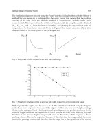
Conduction with Resistances in Series A steady-state temperature profile in a planar composite wall, with three constant thermal
conductivities and no source terms, is shown in Fig. 5-3a. The corresponding thermal circuit is given in Fig. 5-3b. The rate of heat transfer through each of the layers is the same. The total resistance is the
sum of the individual resistances shown in Fig. 5-3b:
T1 − T2
T1 − T2
Q. = ᎏᎏᎏᎏ
= ᎏᎏ
∆XA
∆XB
∆XC
RA + RB + RC
ᎏᎏ + ᎏᎏ + ᎏᎏ
kAA
kBA
kCA
(5-9)
Additional resistances in the series may occur at the surfaces of the
solid if they are in contact with a fluid. The rate of convective heat
transfer, between a surface of area A and a fluid, is represented by
Newton’s law of cooling as
.
Tsurface − Tfluid
Q = hA(Tsurface − Tfluid) = ᎏᎏ
(5-10)
1ր(hA)
where 1/(hA) is the resistance due to convection (K/W) and the heattransfer coefficient is h[Wր(m2⋅K)]. For the cylindrical geometry
shown in Fig. 5-2, with convection to inner and outer fluids at temperatures Ti and To, with heat-transfer coefficients hi and ho, the
steady-state rate of heat transfer is
.
Q=
Ti − To
Ti − To
= ᎏᎏ
ln(r2րr1)
Ri + R1 + Ro
1
1
ᎏ + ᎏ + ᎏ
2πkL
2πr1Lhi
2πr2Lho
(5-11)
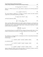
Example 1: Conduction with Resistances in Series and Parallel Figure 5-4 shows the thermal circuit for a furnace wall. The outside surface has a known temperature T2 = 625 K. The temperature of the surroundings
B
T1
T2
(a)
Ti1
Ti2
T2
∆ xA
∆x B
∆ xC
kA A
kBA
kC A
(b)
Steady-state temperature profile in a composite wall with constant
thermal conductivities kA, kB, and kC and no energy sources in the wall. The thermal circuit is shown in (b). The total resistance is the sum of the three resistances shown.
FIG. 5-3
T2
∆ xD
∆x B
∆ xS
kD
kB
kS
Tsur
1
hR
FIG. 5-4 Thermal circuit for Example 1. Steady-state conduction in a furnace
wall with heat losses from the outside surface by convection (hC) and radiation
(hR) to the surroundings at temperature Tsur. The thermal conductivities kD, kB,
and kS are constant, and there are no sources in the wall. The heat flux q has
units of W/m2.
Tsur is 290 K. We want to estimate the temperature of the inside wall T1. The wall
consists of three layers: deposit [kD = 1.6 Wր(m⋅K), ∆xD = 0.080 m], brick
[kB = 1.7 Wր(m⋅K), ∆xB = 0.15 m], and steel [kS = 45 Wր(m⋅K), ∆xS = 0.00254 m].
The outside surface loses heat by two parallel mechanisms—convection and
radiation. The convective heat-transfer coefficient hC = 5.0 Wր(m2⋅K). The
radiative heat-transfer coefficient hR = 16.3 Wր(m2⋅K). The latter is calculated
from
hR = ε2σ(T22 + T2sur)(T2 + Tsur)
(5-12)
where the emissivity of surface 2 is ε2 = 0.76 and the Stefan-Boltzmann constant σ = 5.67 × 10⁻⁸ Wր(m2⋅K4).
Referring to Fig. 5-4, the steady-state heat flux q (W/m2) through the wall is
.
T1 Ϫ T2
Q
q = ᎏ = ᎏᎏ = (hC + hR)(T2 − Tsur)
∆XD ∆XB ∆XS
A
ᎏ
ᎏᎏ + ᎏᎏ + ᎏᎏ
kD
kB
kS
Solving for T1 gives
∆xD
∆xB
∆xS
T1 = T2 + ᎏ + ᎏ + ᎏ (hC + hR)(T2 − Tsur)
kD
kB
kS
0.080
0.15
0.00254
T1 = 625 + ᎏ + ᎏ + ᎏ (5.0 + 16.3)(625 − 290) = 1610 K
1.6
1.7
45
Conduction with Heat Source Application of the law of conservation of energy to a one-dimensional solid, with the heat flux given
by (5-1) and volumetric source term S (W/m3), results in the following
equations for steady-state conduction in a flat plate of thickness 2R
(b = 1), a cylinder of diameter 2R (b = 2), and a sphere of diameter 2R
(b = 3). The parameter b is a measure of the curvature. The thermal
conductivity is constant, and there is convection at the surface, with
heat-transfer coefficient h and fluid temperature T∞.
Q
T1
T1
hc
d
dT
S
ᎏ rb−1 ᎏ + ᎏ rb−1 = 0
dr
dr
k
.
C
1
.
=Q/A
and
where resistances Ri and Ro are the convective resistances at the inner
and outer surfaces. The total resistance is again the sum of the resistances in series.
A
q
5-5
dT(0)
ᎏ =0
dr
(symmetry condition)
(5-13)
dT
−k ᎏ = h[T(R) − T∞]
dr
The solutions to (5-13), for uniform S, are
T(r) Ϫ T∞
1
r
ᎏᎏ
ϭᎏ 1 Ϫ ᎏ
SR2րk
2b
R
΄ ΅ϩ ᎏ
bBi
2
1
Ά
b ϭ 1, plate, thickness 2R
b ϭ 2, cylinder, diameter 2R
b ϭ 3, sphere, diameter 2R
(5-14)
where Bi = hR/k is the Biot number. For Bi << 1, the temperature in
the solid is uniform. For Bi >> 1, the surface temperature T(R) ϭ T∞.
Two- and Three-Dimensional Conduction Application of the
law of conservation of energy to a three-dimensional solid, with the
5-6
HEAT AND MASS TRANSFER
heat flux given by (5-1) and volumetric source term S (W/m3), results
in the following equation for steady-state conduction in rectangular
coordinates.
∂
∂T
∂
∂T
∂
∂T
ᎏ kᎏ + ᎏ kᎏ + ᎏ kᎏ + S = 0
∂x
∂x
∂y
∂y
∂z
∂z
(5-15)
Similar equations apply to cylindrical and spherical coordinate systems. Finite difference, finite volume, or finite element methods are
generally necessary to solve (5-15). Useful introductions to these
numerical techniques are given in the General References and Sec. 3.
Simple forms of (5-15) (constant k, uniform S) can be solved analytically. See Arpaci, Conduction Heat Transfer, Addison-Wesley, 1966,
p. 180, and Carslaw and Jaeger, Conduction of Heat in Solids, Oxford
University Press, 1959. For problems involving heat flow between two
surfaces, each isothermal, with all other surfaces being adiabatic, the
shape factor approach is useful (Mills, Heat Transfer, 2d ed., PrenticeHall, 1999, p. 164).
UNSTEADY-STATE CONDUCTION
Application of the law of conservation of energy to a three-dimensional solid, with the heat flux given by (5-1) and volumetric source
term S (W/m3), results in the following equation for unsteady-state
conduction in rectangular coordinates.
∂T
∂
∂T
∂
∂T
∂
∂T
ρc ᎏ = ᎏ k ᎏ + ᎏ k ᎏ + ᎏ k ᎏ + S
∂t
∂x
∂x
∂y
∂y
∂z
∂z
(5-16)
The energy storage term is on the left-hand side, and ρ and c are the
density (kg/m3) and specific heat [Jր(kg и K)]. Solutions to (5-16) are
generally obtained numerically (see General References and Sec. 3).
The one-dimensional form of (5-16), with constant k and no source
term, is
∂T
∂2T
ᎏ = αᎏ
∂t
∂x2
(5-17)
where α ϭ kր(ρc) is the thermal diffusivity (m2/s).
One-Dimensional Conduction: Lumped and Distributed
Analysis The one-dimensional transient conduction equations in
rectangular (b = 1), cylindrical (b = 2), and spherical (b = 3) coordinates, with constant k, initial uniform temperature Ti, S = 0, and convection at the surface with heat-transfer coefficient h and fluid
temperature T∞, are
α ∂ bϪ1 ∂T
∂T
ᎏϭᎏ
ᎏ r ᎏ
rbϪ1 ∂r
∂t
∂r
for t Ͻ 0,
at r ϭ 0,
at r ϭ R,
Ά
b ϭ 1, plate, thickness 2R
b ϭ 2, cylinder, diameter 2R
b ϭ 3, sphere, diameter 2R
and
Plate
Cylinder
Sphere
A1
B1
S1
2sinδ1
ᎏᎏ
δ1 + sinδ1cosδ1
2Bi2
ᎏᎏ
2
2
δ1(Bi + Bi + δ21)
cos(δ1ζ)
2J1(δ1)
ᎏᎏ
δ1[J20(δ1) + J21(δ1)]
4Bi2
ᎏᎏ
2 2
δ1(δ1 + Bi2)
J0(δ1ζ)
2Bi[δ21 + (Bi − 1)2]1ր2
ᎏᎏᎏ
δ21 + Bi2 − Bi
6Bi2
ᎏᎏ
δ21(δ21 + Bi2 − Bi)
sinδ1ζ
ᎏ
δ1ζ
The time scale is the time required for most of the change in θրθi or
Q/Qi to occur. When t = τ, θրθi = exp(−1) = 0.368 and roughly twothirds of the possible change has occurred.
When a lumped analysis is not valid (Bi > 0.2), the single-term solutions to (5-18) are convenient:
θ
Q
ᎏ = A1 exp (− δ21Fo)S1(δ1ζ) and ᎏ = 1 − B1 exp (−δ21Fo) (5-21)
θi
Qi
where the first Fourier coefficients A1 and B1 and the spatial functions
S1 are given in Table 5-1. The first eigenvalue δ1 is given by (5-22) in
conjunction with Table 5-2. The one-term solutions are accurate to
within 2 percent when Fo > Foc. The values of the critical Fourier
number Foc are given in Table 5-2.
The first eigenvalue is accurately correlated by (Yovanovich, Chap.
3 of Rohsenow, Hartnett, and Cho, Handbook of Heat Transfer, 3d
ed., McGraw-Hill, 1998, p. 3.25)
δ1,∞
δ1 ϭ ᎏᎏ
(5-22)
[1 ϩ (δ1,∞րδ1,0)n]1րn
Equation (5-22) gives values of δ1 that differ from the exact values by
less than 0.4 percent, and it is valid for all values of Bi. The values of
δ1,∞, δ1,0, n, and Foc are given in Table 5-2.
Example 2: Correlation of First Eigenvalues by Eq. (5-22) As
an example of the use of Eq. (5-22), suppose that we want δ1 for the flat plate
ෆ ϭ ͙5ෆ, and n = 2.139. Equawith Bi = 5. From Table 5-2, δ1,∞ ϭ πր2, δ1,0 ϭ ͙Bi
tion (5-22) gives
πր2
δ1 ϭ ᎏᎏᎏ
ϭ 1.312
[1 ϩ (πր2/͙5
ෆ)2.139]1ր2.139
Example 3: One-Dimensional, Unsteady Conduction Calcula-
(5-18)
The solutions to (5-18) can be compactly expressed by using dimensionless variables: (1) temperature θրθi = [T(r,t) − T∞]ր(Ti − T∞); (2)
heat loss fraction QրQi = Qր[ρcV(Ti − T∞)], where V is volume; (3) distance from center ζ = rրR; (4) time Fo = αtրR2; and (5) Biot number Bi =
hR/k. The temperature and heat loss are functions of ζ, Fo, and Bi.
When the Biot number is small, Bi < 0.2, the temperature of the
solid is nearly uniform and a lumped analysis is acceptable. The solution to the lumped analysis of (5-18) is
Geometry
The tabulated value is 1.3138.
T ϭ Ti
(initial temperature)
∂T
(symmetry condition)
ᎏ ϭ0
∂r
∂T
Ϫ k ᎏ ϭ h(T Ϫ T∞)
∂r
θ
hA
ᎏ = exp − ᎏ t
θi
ρcV
TABLE 5-1 Fourier Coefficients and Spatial Functions for Use
in Eqs. (5-21)
Q
hA
ᎏ = 1 − exp − ᎏ t
Qi
ρcV
(5-19)
where A is the active surface area and V is the volume. The time scale
for the lumped problem is
ρcV
τ= ᎏ
(5-20)
hA
tion As an example of the use of Eq. (5-21), Table 5-1, and Table 5-2, consider the cooking time required to raise the center of a spherical, 8-cm-diameter
dumpling from 20 to 80°C. The initial temperature is uniform. The dumpling is
heated with saturated steam at 95°C. The heat capacity, density, and thermal
conductivity are estimated to be c = 3500 Jր(kgиK), ρ = 1000 kgրm3, and k = 0.5
Wր(mиK), respectively.
Because the heat-transfer coefficient for condensing steam is of order 104, the Bi
→ ∞ limit in Table 5-2 is a good choice and δ1 = π. Because we know the desired
temperature at the center, we can calculate θրθi and then solve (5-21) for the time.
80 − 95
θ
T(0,t) − T∞
ᎏ = ᎏᎏ
= ᎏ = 0.200
20 − 95
θi
Ti − T∞
For Bi → ∞, A1 in Table 5-1 is 2 and for ζ = 0, S1 in Table 5-1 is 1. Equation
(5-21) becomes
αt
θ
ᎏ = 2 exp (−π2Fo) = 2 exp −π2 ᎏ2
R
θi
TABLE 5-2 First Eigenvalues for Bi Æ 0 and Bi Æ • and
Correlation Parameter n
The single-term approximations apply only if Fo ≥ Foc.
Geometry
Bi → 0
Bi → ∞
n
Foc
Plate
Cylinder
Sphere
δ1 → ͙Bi
ෆ
δ1 → ͙2Bi
ෆ
δ1 → ͙3Bi
ෆ
δ1 → πր2
δ1 → 2.4048255
δ1 → π
2.139
2.238
2.314
0.24
0.21
0.18
HEAT TRANSFER BY CONVECTION
where erf(z) is the error function. The depth to which the heat penetrates in time t is approximately (12αt)1ր2.
If the heat-transfer coefficient is finite,
Solving for t gives the desired cooking time.
θ
R
(0.04 m)
0.2
t = − ᎏ2 ln ᎏ = − ᎏᎏᎏ ln ᎏ = 43.5 min
2θi
απ
1.43 × 10⁻⁷(m2րs)π2
2
2
2
Example 4: Rule of Thumb for Time Required to Diffuse a
Distance R A general rule of thumb for estimating the time required to diffuse a distance R is obtained from the one-term approximations. Consider the
equation for the temperature of a flat plate of thickness 2R in the limit as Bi →
∞. From Table 5-2, the first eigenvalue is δ1 = πր2, and from Table 5-1,
θ
π
ᎏ = A1 exp − ᎏ
θi
2
αt
ᎏ2 cosδ1ζ
R
΄ ΅
2
When t ϭ R2րα, the temperature ratio at the center of the plate (ζ ϭ 0) has
decayed to exp(Ϫπ2ր4), or 8 percent of its initial value. We conclude that diffusion through a distance R takes roughly R2րα units of time, or alternatively, the
distance diffused in time t is about (αt)1ր2.
One-Dimensional Conduction: Semi-infinite Plate Consider
a semi-infinite plate with an initial uniform temperature Ti. Suppose
that the temperature of the surface is suddenly raised to T∞; that is, the
heat-transfer coefficient is infinite. The unsteady temperature of the
plate is
T(x,t) − T∞
x
ᎏᎏ = erf ᎏ
Ti − T∞
2͙ෆ
αt
5-7
(5-23)
T(x,t)ϪT∞
ᎏᎏ
Ti Ϫ T∞
x
x
h͙αt
ෆ
hx h2αt
= erfc ᎏ −exp ᎏ + ᎏ
erfc ᎏ + ᎏ
k
k2
2͙ෆ
αt
k
2͙αt
ෆ
(5-24)
where erfc(z) is the complementary error function. Equations (5-23)
and (5-24) are both applicable to finite plates provided that their halfthickness is greater than (12αt)1ր2.
Two- and Three-Dimensional Conduction The one-dimensional solutions discussed above can be used to construct solutions to
multidimensional problems. The unsteady temperature of a rectangular, solid box of height, length, and width 2H, 2L, and 2W, respectively, with governing equations in each direction as in (5-18), is
θ
ᎏθ
i
2Hϫ2Lϫ2W
θ
= ᎏ
θi
θ
θ
ᎏθ ᎏθ
2H
i
2L
i
(5-25)
2W
Similar products apply for solids with other geometries, e.g., semiinfinite, cylindrical rods.
HEAT TRANSFER BY CONVECTION
CONVECTIVE HEAT-TRANSFER COEFFICIENT
Convection is the transfer of energy by conduction and radiation in
moving, fluid media. The motion of the fluid is an essential part of
convective heat transfer. A key step in calculating the rate of heat
transfer by convection is the calculation of the heat-transfer coefficient. This section focuses on the estimation of heat-transfer coefficients for natural and forced convection. The conservation equations
for mass, momentum, and energy, as presented in Sec. 6, can be used
to calculate the rate of convective heat transfer. Our approach in this
section is to rely on correlations.
In many cases of industrial importance, heat is transferred from one
fluid, through a solid wall, to another fluid. The transfer occurs in a
heat exchanger. Section 11 introduces several types of heat exchangers,
design procedures, overall heat-transfer coefficients, and mean temperature differences. Section 3 introduces dimensional analysis and
the dimensionless groups associated with the heat-transfer coefficient.
Individual Heat-Transfer Coefficient The local rate of convective heat transfer between a surface and a fluid is given by Newton’s law of cooling
q ϭ h(Tsurface Ϫ Tfluid)
(5-26)
where h [Wր(m2иK)] is the local heat-transfer coefficient and q is the
energy flux (W/m2). The definition of h is arbitrary, depending on
whether the bulk fluid, centerline, free stream, or some other temperature is used for Tfluid. The heat-transfer coefficient may be defined
on an average basis as noted below.
Consider a fluid with bulk temperature T, flowing in a cylindrical
tube of diameter D, with constant wall temperature Ts. An energy balance on a short section of the tube yields
. dT
cpm ᎏ ϭ πDh(Ts Ϫ T)
dx
(5-27)
.
where cp is the specific heat at constant pressure [Jր(kgиK)], m is the
mass flow rate (kg/s), and x is the distance from the inlet. If the temperature of the fluid at the inlet is Tin, the temperature of the fluid at
a downstream distance L is
⎯
T(L) Ϫ Ts
hπDL
(5-28)
ᎏᎏ ϭ exp Ϫ ᎏ
.
Tin Ϫ Ts
m cp
⎯
The average heat-transfer coefficient h is defined by
⎯ 1 L
(5-29)
h = ᎏ h dx
L 0
Overall Heat-Transfer Coefficient and Heat Exchangers A
local, overall heat-transfer coefficient U for the cylindrical geometry
shown in Fig. 5-2 is defined by using Eq. (5-11) as
.
Q
Ti − To
ᎏ = ᎏᎏᎏ = 2πr1U(Ti − To) (5-30)
1 + ln(r2րr1) + 1
∆x
ᎏᎏ ᎏᎏ ᎏᎏ
2πr1hi
2πk
2πr2ho
where ∆x is a short length of tube in the axial direction. Equation
(5-30) defines U by using the inside perimeter 2πr1. The outer
perimeter can also be used. Equation (5-30) applies to clean tubes.
Additional resistances are present in the denominator for dirty
tubes (see Sec. 11).
For counterflow and parallel flow heat exchanges, with high- and
low-temperature fluids (TH and TC) and flow directions as defined in
Fig. 5-5, the total heat transfer for the exchanger is given by
.
Q = UA ∆Tlm
(5-31)
where A is the area for heat exchange and the log mean temperature
difference ∆Tlm is defined as
(TH − TC)L − (TH − TL)0
∆Tlm = ᎏᎏᎏ
(5-32)
ln[(TH − TC)L − (TH − TL)0]
Equation (5-32) applies to both counterflow and parallel flow exchangers with the nomenclature defined in Fig. 5-5. Correction factors to
∆Tlm for various heat exchanger configurations are given in Sec. 11.
In certain applications, the log mean temperature difference is
replaced with an arithmetic mean difference:
(TH − TC)L + (TH − TL)0
∆Tam = ᎏᎏᎏ
(5-33)
2
Average heat-transfer coefficients are occasionally reported based on
Eqs. (5-32) and (5-33) and are written as hlm and ham.
Representation of Heat-Transfer Coefficients Heat-transfer
coefficients are usually expressed in two ways: (1) dimensionless relations and (2) dimensional equations. Both approaches are used below.
The dimensionless form of the heat-transfer coefficient is the Nusselt
͵
5-8
HEAT AND MASS TRANSFER
For horizontal flat surfaces, the characteristic dimension for the
correlations is [Goldstein, Sparrow, and Jones, Int. J. Heat Mass
Transfer, 16, 1025–1035 (1973)]
A
Lϭ ᎏ
(5-37)
p
TH
TC
x=0
x=L
where A is the area of the surface and p is the perimeter. With hot surfaces facing upward, or cold surfaces facing downward [Lloyd and
Moran, ASME Paper 74-WA/HT-66 (1974)],
(a)
⎯⎯ ϭ
NuL
TH
TC
x=0
104 Ͻ RaL Ͻ 107
(5-38)
0.15Ra1ր3
L
107 Ͻ RaL Ͻ 1010
(5-39)
and for hot surfaces facing downward, or cold surfaces facing upward,
⎯⎯
NuL ϭ 0.27Ra1ր4
105 Ͻ RaL Ͻ 1010
(5-40)
L
x=L
(b)
Nomenclature for (a) counterflow and (b) parallel flow heat exchangers for use with Eq. (5-32).
FIG. 5-5
number. For example, with a cylinder of diameter D in cross flow, the
local Nusselt number is defined as NuD = hD/k, where k is the thermal
conductivity of the fluid. The subscript D is important because different characteristic lengths can be used to define Nu. The average Nus⎯⎯
⎯
selt number is written NuD ϭ hDրk.
NATURAL CONVECTION
Natural convection occurs when a fluid is in contact with a solid surface
of different temperature. Temperature differences create the density
gradients that drive natural or free convection. In addition to the Nusselt number mentioned above, the key dimensionless parameters for
natural convection include the Rayleigh number Rax ϭ β ∆T gx3ր
να and the Prandtl number Pr ϭ νրα. The properties appearing in Ra
and Pr include the volumetric coefficient of expansion β (KϪ1); the difference ∆T between the surface (Ts) and free stream (Te) temperatures (K or °C); the acceleration of gravity g(m/s2); a characteristic
dimension x of the surface (m); the kinematic viscosity ν(m2րs); and
the thermal diffusivity α(m2րs). The volumetric coefficient of expansion for an ideal gas is β = 1րT, where T is absolute temperature. For a
given geometry,
⎯⎯
(5-34)
Nux ϭ f(Rax, Pr)
External Natural Flow for Various Geometries For vertical
walls, Churchill and Chu [Int. J. Heat Mass Transfer, 18, 1323 (1975)]
recommend, for laminar and turbulent flow on isothermal, vertical
walls with height L,
0.387Ra1ր6
⎯⎯
L
NuL ϭ 0.825 ϩ ᎏᎏᎏ
[1 ϩ (0.492րPr)9ր16]8ր27
Ά
·
2
(5-35)
⎯⎯
⎯
where the fluid properties for Eq. (5-35) and NuL ϭ hLրk are evaluated at the film temperature Tf = (Ts + Te)/2. This correlation is valid
for all Pr and RaL. For vertical cylinders with boundary layer thickness
much less than their diameter, Eq. (5-35) is applicable. An expression
for uniform heating is available from the same reference.
For laminar and turbulent flow on isothermal, horizontal cylinders
of diameter D, Churchill and Chu [Int. J. Heat Mass Transfer, 18,
1049 (1975)] recommend
⎯⎯
0.387Ra1ր6
D
NuL ϭ 0.60 ϩ ᎏᎏᎏ
[1 ϩ (0.559րPr)9ր16]8ր27
Ά
Ά
0.54Ra1ր4
L
·
2
(5-36)
Fluid properties for (5-36) should be evaluated at the film temperature Tf = (Ts + Te)/2. This correlation is valid for all Pr and RaD.
Fluid properties for Eqs. (5-38) to (5-40) should be evaluated at the
film temperature Tf = (Ts + Te)/2.
Simultaneous Heat Transfer by Radiation and Convection
Simultaneous heat transfer by radiation and convection is treated per
the procedure outlined in Examples 1 and 5. A radiative heat-transfer
coefficient hR is defined by (5-12).
Mixed Forced and Natural Convection Natural convection is
commonly assisted or opposed by forced flow. These situations are
discussed, e.g., by Mills (Heat Transfer, 2d ed., Prentice-Hall, 1999,
p. 340) and Raithby and Hollands (Chap. 4 of Rohsenow, Hartnett, and
Cho, Handbook of Heat Transfer, 3d ed., McGraw-Hill, 1998, p. 4.73).
Enclosed Spaces The rate of heat transfer across an enclosed
space is described in terms of a heat-transfer coefficient based on the
temperature difference between two surfaces:
.
⎯
QրA
hϭ ᎏ
(5-41)
TH Ϫ TC
For rectangular cavities, the plate spacing between the two surfaces L
is the characteristic dimension that defines the Nusselt and Rayleigh
numbers. The temperature difference in the Rayleigh number,
RaL ϭ β ∆T gL3րνα is ∆T ϭ TH Ϫ TC.
For a horizontal rectangular cavity heated from below, the onset of
advection requires RaL > 1708. Globe and Dropkin [J. Heat Transfer,
81, 24–28 (1959)] propose the correlation
⎯⎯
0.074
NuL ϭ 0.069Ra1ր3
3 × 10⁵ < RaL < 7 × 10⁹ (5-42)
L Pr
All properties in (5-42) are calculated at the average temperature
(TH + TC)/2.
For vertical rectangular cavities of height H and spacing L, with
Pr ≈ 0.7 (gases) and 40 < H/L < 110, the equation of Shewen et al. [J.
Heat Transfer, 118, 993–995 (1996)] is recommended:
Ά
⎯⎯
0.0665Ra1ր3
L
NuL ϭ 1 ϩ ᎏᎏ
1 ϩ (9000րRaL)1.4
΄
΅·
2
1ր2
RaL < 106
(5-43)
All properties in (5-43) are calculated at the average temperature
(TH + TC)/2.
Example 5: Comparison of the Relative Importance of Natural
Convection and Radiation at Room Temperature Estimate the
heat losses by natural convection and radiation for an undraped person standing
in still air. The temperatures of the air, surrounding surfaces, and skin are 19, 15,
and 35°C, respectively. The height and surface area of the person are 1.8 m and
1.8 m2. The emissivity of the skin is 0.95.
We can estimate the Nusselt number by using (5-35) for a vertical, flat plate
of height L = 1.8 m. The film temperature is (19 + 35)ր2 = 27°C. The Rayleigh
number, evaluated at the film temperature, is
(1ր300)(35 − 19)9.81(1.8)3
β ∆T gL3
RaL = ᎏ = ᎏᎏᎏ
= 8.53 × 10⁹
1.589 × 10⁻⁵(2.25 × 10⁻⁵)
να
From (5-35) with Pr = 0.707, the Nusselt number is 240 and the average heattransfer coefficient due to natural convection is
W
⎯ k ⎯⎯
0.0263
h = ᎏ NuL = ᎏ (240) = 3.50 ᎏ
m2иK
L
1.8
HEAT TRANSFER BY CONVECTION
TABLE 5-3 Effect of Entrance Configuration on Values of C
and n in Eq. (5-53) for Pr ª 1 (Gases and Other Fluids with Pr
about 1)
The radiative heat-transfer coefficient is given by (5-12):
hR = εskinσ(T2skin + T2sur)(Tskin + Tsur)
W
= 0.95(5.67 × 10⁻⁸)(3082 + 2882)(308 + 288) = 5.71 ᎏ
m2⋅K
The total rate of heat loss is
. ⎯
⎯
Q = hA(Tskin − Tair) + hRA(Tskin − Tsur)
Entrance configuration
= 3.50(1.8)(35 − 19) + 5.71(1.8)(35 − 15) = 306 W
At these conditions, radiation is nearly twice as important as natural convection.
FORCED CONVECTION
Forced convection heat transfer is probably the most common mode
in the process industries. Forced flows may be internal or external.
This subsection briefly introduces correlations for estimating heattransfer coefficients for flows in tubes and ducts; flows across plates,
cylinders, and spheres; flows through tube banks and packed beds;
heat transfer to nonevaporating falling films; and rotating surfaces.
Section 11 introduces several types of heat exchangers, design procedures, overall heat-transfer coefficients, and mean temperature differences.
Flow in Round Tubes In addition to the Nusselt (NuD = hD/k)
and Prandtl (Pr = νրα) numbers introduced above, the key dimensionless parameter for forced convection in round tubes of diameter D
is the. Reynolds number Re = GDրµ, where G is the mass velocity
G = m րAc and Ac is the cross-sectional area Ac = πD2ր4. For internal
flow in a tube or duct, the heat-transfer coefficient is defined as
q = h(Ts − Tb)
(5-44)
where Tb is the bulk or mean temperature at a given cross section and
Ts is the corresponding surface temperature.
For laminar flow (ReD < 2100) that is fully developed, both hydrodynamically and thermally, the Nusselt number has a constant value.
For a uniform wall temperature, NuD = 3.66. For a uniform heat flux
through the tube wall, NuD = 4.36. In both cases, the thermal conductivity of the fluid in NuD is evaluated at Tb. The distance x required for
a fully developed laminar velocity profile is given by [(xրD)րReD] ≈
0.05. The distance x required for fully developed velocity and thermal
profiles is obtained from [(x/D)ր(ReD Pr)] ≈ 0.05.
For a constant wall temperature, a fully developed laminar velocity
profile, and a developing thermal profile, the average Nusselt number
is estimated by [Hausen, Allg. Waermetech., 9, 75 (1959)]
⎯⎯
0.0668(DրL) ReD Pr
NuD = 3.66 + ᎏᎏᎏ
(5-45)
1 + 0.04[(DրL) ReD Pr]2ր3
For large values of L, Eq. (5-45) approaches NuD = 3.66. Equation (545) also applies to developing velocity and thermal profiles conditions
if Pr >>1. The properties in (5-45) are evaluated at the bulk mean
temperature
⎯
Tb = (Tb,in + Tb,out)ր2
(5-46)
For a constant wall temperature with developing laminar velocity
and thermal profiles, the average Nusselt number is approximated by
[Sieder and Tate, Ind. Eng. Chem., 28, 1429 (1936)]
1ր3 µ
0.14
⎯⎯
D
b
NuD = 1.86 ᎏ ReD Pr
(5-47)
ᎏ
µs
L
The properties, except for µs, are evaluated at the bulk mean temperature per (5-46) and 0.48 < Pr < 16,700 and 0.0044 < µb րµs < 9.75.
For fully developed flow in the transition region between laminar
and turbulent flow, and for fully developed turbulent flow, Gnielinski’s
[Int. Chem. Eng., 16, 359 (1976)] equation is recommended:
(fր2)(ReD − 1000)(Pr)
NuD = ᎏᎏᎏ
K
(5-48)
1 + 12.7(fր2)1ր2 (Pr2ր3 − 1)
where 0.5 < Pr < 105, 2300 < ReD < 106, K = (Prb/Prs)0.11 for liquids
(0.05 < Prb/Prs < 20), and K = (Tb/Ts)0.45 for gases (0.5 < Tb/Ts < 1.5).
The factor K corrects for variable property effects. For smooth tubes,
the Fanning friction factor f is given by
f = 0.25(0.790 ln ReD − 1.64)−2
2300 < ReD < 106
5-9
(5-49)
Long calming section
Open end, 90° edge
180° return bend
90° round bend
90° elbow
C
n
0.9756
2.4254
0.9759
1.0517
2.0152
0.760
0.676
0.700
0.629
0.614
For rough pipes, approximate values of NuD are obtained if f is estimated by the Moody diagram of Sec. 6. Equation (5-48) is corrected
for entrance effects per (5-53) and Table 5-3. Sieder and Tate [Ind.
Eng. Chem., 28, 1429 (1936)] recommend a simpler but less accurate
equation for fully developed turbulent flow
µb
1ր3
NuD = 0.027 Re4ր5
ᎏ
D Pr
µs
0.14
(5-50)
where 0.7 < Pr < 16,700, ReD < 10,000, and L/D > 10. Equations (548) and (5-50) apply to both constant temperature and uniform heat
flux along the tube. The properties are evaluated at the bulk temperature Tb, except for µs, which is at the temperature of the tube. For
L/D⎯greater
than about 10, Eqs. (5-48) and (5-50) provide an estimate
⎯
of NuD. In this case, the properties are evaluated at the bulk mean
temperature per (5-46). More complicated and comprehensive predictions of fully developed turbulent convection are available in
Churchill and Zajic [AIChE J., 48, 927 (2002)] and Yu, Ozoe, and
Churchill [Chem. Eng. Science, 56, 1781 (2001)].
For fully developed turbulent flow of liquid metals, the Nusselt number depends on the wall boundary condition. For a constant wall temperature [Notter and Sleicher, Chem. Eng. Science, 27, 2073 (1972)],
0.93
NuD = 4.8 + 0.0156 Re0.85
D Pr
(5-51)
while for a uniform wall heat flux,
0.93
NuD = 6.3 + 0.0167 Re0.85
D Pr
(5-52)
In both cases the properties are evaluated at Tb and 0.004 < Pr < 0.01
and 104 < ReD < 106.
Entrance effects for turbulent flow with simultaneously developing
velocity and thermal profiles can be significant when L/D < 10. Shah
and Bhatti correlated entrance effects for gases (Pr ≈ 1) to give an
equation for the average Nusselt number in the entrance region (in
Kaka, Shah, and Aung, eds., Handbook of Single-Phase Convective
Heat Transfer, Chap. 3, Wiley-Interscience, 1987).
⎯⎯
NuD
C
(5-53)
ᎏ = 1 + ᎏn
NuD
(xրD)
where NuD is the fully developed Nusselt number and the constants C
and n are given in Table 5-3 (Ebadian and Dong, Chap. 5 of
Rohsenow, Hartnett, and Cho, Handbook of Heat Transfer, 3d ed.,
McGraw-Hill, 1998, p. 5.31). The tube entrance configuration determines the values of C and n as shown in Table 5-3.
Flow in Noncircular Ducts The length scale in the Nusselt and
Reynolds numbers for noncircular ducts is the hydraulic diameter,
Dh = 4Ac/p, where Ac is the cross-sectional area for flow and p is the
wetted perimeter. Nusselt numbers for fully developed laminar flow
in a variety of noncircular ducts are given by Mills (Heat Transfer, 2d
ed., Prentice-Hall, 1999, p. 307). For turbulent flows, correlations for
round tubes can be used with D replaced by Dh.
For annular ducts, the accuracy of the Nusselt number given by
(5-48) is improved by the following multiplicative factors [Petukhov
and Roizen, High Temp., 2, 65 (1964)].
Di −0.16
Inner tube heated 0.86 ᎏ
Do
Di 0.6
1 − 0.14 ᎏ
Do
where Di and Do are the inner and outer diameters, respectively.
Outer tube heated
5-10
HEAT AND MASS TRANSFER
Example 6: Turbulent Internal Flow Air at 300 K, 1 bar, and 0.05
kg/s enters a channel of a plate-type heat exchanger (Mills, Heat Transfer, 2d
ed., Prentice-Hall, 1999) that measures 1 cm wide, 0.5 m high, and 0.8 m long.
The walls are at 600 K, and the mass flow rate is 0.05 kg/s. The entrance has a
90° edge. We want to estimate the exit temperature of the air.
Our approach will use (5-48) to estimate the average heat-transfer coefficient, followed by application of (5-28) to calculate the exit temperature. We
assume ideal gas behavior and an exit temperature of 500 K. The estimated bulk
mean temperature of the air is, by (5-46), 400 K. At this temperature, the properties of the air are Pr = 0.690, µ = 2.301 × 10⁻⁵ kgր(m⋅s), k = 0.0338 Wր(m⋅K),
and cp = 1014 Jր(kg⋅K).
We start by calculating the hydraulic diameter Dh = 4Ac/p. The cross-sectional
area for flow Ac is 0.005 m2, and the wetted perimeter p is 1.02 m. The hydraulic
diameter Dh = 0.01961 m. The Reynolds number is
.
m Dh
0.05(0.01961)
ReD = ᎏ
= ᎏᎏᎏ
= 8521
Acµ
0.005(2.301 × 10⁻⁵)
External Flows For a single cylinder in cross flow, Churchill and
Bernstein recommend [J. Heat Transfer, 99, 300 (1977)]
1ր3
5ր8 4ր5
0.62 Re1ր2
⎯⎯
ReD
D Pr
NuD = 0.3 + ᎏᎏ
1+ ᎏ
(5-56)
2ր3 1ր4
[1 + (0.4րPr) ]
282,000
⎯⎯
⎯
where NuD = hDրk. Equation (5-56) is for all values of ReD and Pr,
provided that ReD Pr > 0.4. The fluid properties are evaluated at the
film temperature (Te + Ts)/2, where Te is the free-stream temperature
and Ts is the surface temperature. Equation (5-56)
also applies to the uni⎯
form heat flux boundary condition provided h is based on the perimeteraveraged temperature difference between Ts and Te.
For an isothermal spherical surface, Whitaker recommends
[AIChE, 18, 361 (1972)]
1ր4
⎯⎯
0.4 µe
2ր3
NuD = 2 + (0.4Re1ր2
(5-57)
ᎏ
D + 0.06ReD )Pr
µs
This equation is based on data for 0.7 < Pr < 380, 3.5 < ReD < 8 × 10⁴,
and 1 < (µeրµs) < 3.2. The properties are evaluated at the free-stream
temperature Te, with the exception of µs, which is evaluated at the surface temperature Ts.
The average Nusselt number for laminar flow over an isothermal
flat plate of length x is estimated from [Churchill and Ozoe, J. Heat
Transfer, 95, 416 (1973)]
⎯⎯
1.128 Pr1ր2 Re1ր2
x
Nux = ᎏᎏᎏ
(5-58)
[1 + (0.0468րPr)2ր3]1ր4
΄
h
The flow is in the transition region, and Eqs. (5-49) and (5-48) apply:
f = 0.25(0.790 ln ReD − 1.64) = 0.25(0.790 ln 8521 − 1.64) = 0.008235
−2
−2
h
(fր2)(ReD − 1000)(Pr)
NuD = ᎏᎏᎏ
K
1 + 12.7(fր2)1ր2(Pr2ր3 − 1)
(0.008235ր2)(8521 − 1000)(0.690) 400
ᎏ
= ᎏᎏᎏᎏ
1 + 12.7(0.008235ր2)1ր2 (0.6902ր3 − 1) 600
0.45
= 21.68
Entrance effects are included by using (5-53) for an open end, 90° edge:
⎯⎯
C
2.4254
(21.68) = 25.96
NuD = 1 + ᎏn NuD = 1 + ᎏᎏ
(xրD)
(0.8ր0.01961)0.676
The average heat-transfer coefficient becomes
W
⎯
0.0338
k ⎯⎯
h = ᎏ NuD = ᎏ (25.96) = 44.75 ᎏ
m2⋅K
Dh
0.01961
The exit temperature is calculated from (5-28):
⎯
hpL
T(L) = Ts − (Ts − Tin)exp − ᎏ
.
mcP
΄
΅
΄
΅
This equation is valid for all values of Pr as long as Rex Pr > 100 and Rex
< 5 × 10⁵. The fluid properties are evaluated at the film temperature
(Te + Ts)/2, where Te is the free-stream temperature and Ts is the surface
temperature. For a uniformly heated flat plate, the local Nusselt number is given by [Churchill and Ozoe, J. Heat Transfer, 95, 78 (1973)]
0.886 Pr1ր2 Re1ր2
x
Nux = ᎏᎏᎏ
(5-59)
[1 + (0.0207րPr)2ր3]1ր4
΄
΅
44.75(1.02)0.8
= 600 − (600 − 300)exp − ᎏᎏ = 450 K
0.05(1014)
where again the properties are evaluated at the film temperature.
The average Nusselt number for turbulent flow over a smooth,
isothermal flat plate of length x is given by (Mills, Heat Transfer, 2d
ed., Prentice-Hall, 1999, p. 315)
⎯⎯
Recr 0.8
1ր3
0.43
Nux = 0.664 Re1ր2
+ 0.036 Re0.8
1− ᎏ
(5-60)
cr Pr
x Pr
Rex
The critical Reynolds number Recr is typically taken as 5 × 10⁵, Recr <
Rex < 3 × 10⁷, and 0.7 < Pr < 400. The fluid properties are evaluated at
the film temperature (Te + Ts)/2, where Te is the free-stream temperature and Ts is the surface temperature. Equation (5-60)
⎯ also applies to
the uniform heat flux boundary condition provided h is based on the
average temperature difference between Ts and Te.
Flow-through Tube Banks Aligned and staggered tube banks are
sketched in Fig. 5-6. The tube diameter is D, and the transverse and longitudinal pitches are ST and SL, respectively. The fluid velocity upstream
We conclude that our estimated exit temperature of 500 K is too high. We could
repeat the calculations, using fluid properties evaluated at a revised bulk mean
temperature of 375 K.
΄
Coiled Tubes For turbulent flow inside helical coils, with tube
inside radius a and coil radius R, the Nusselt number for a straight tube
Nus is related to that for a coiled tube Nuc by (Rohsenow, Hartnett, and
Cho, Handbook of Heat Transfer, 3d ed., McGraw-Hill, 1998, p. 5.90)
Nuc
a
a 0.8
(5-54)
ᎏ = 1.0 + 3.6 1 − ᎏ ᎏ
Nus
R
R
where 2 × 10⁴ < ReD < 1.5 × 10⁵ and 5 < R/a < 84. For lower Reynolds
numbers (1.5 × 10³ < ReD < 2 × 10⁴), the same source recommends
Nuc
a
(5-55)
ᎏ = 1.0 + 3.4 ᎏ
Nus
R
D
V∞
ST
D
ST
SL
SL
(a)
(b)
(a) Aligned and (b) staggered tube bank configurations. The fluid velocity upstream of
the tubes is V∞.
FIG. 5-6
΅
΅
HEAT TRANSFER BY CONVECTION
of the tubes is V∞. To estimate the overall heat-transfer coefficient for the
tube bank, Mills proceeds as follows (Heat Transfer, 2d ed., PrenticeHall, 1999, p. 348). The Reynolds number for use in (5-56) is recalculated
with an effective average velocity in the space between adjacent tubes:
⎯
V
ST
ᎏ = ᎏᎏ
(5-61)
V∞
ST − (πր4)D
The heat-transfer coefficient increases from row 1 to about row 5 of
the tube bank. The average Nusselt number for a tube bank with 10 or
more rows is
⎯⎯10+
⎯⎯
NuD = ΦNu1D
(5-62)
⎯⎯
where Φ is an arrangement factor and Nu1D is the Nusselt number for
the first row, calculated by using the velocity in (5-61). The arrangement factor is calculated as follows. Define dimensionless pitches as
PT = ST/D and PL/D and calculate a factor ψ as follows.
π
1− ᎏ
if PL ≥ 1
4PT
ψ=
(5-63)
π
1− ᎏ
if PL < 1
4PTPL
Ά
The arrangement factors are
0.7 SLրST − 0.3
ᎏᎏ
Φaligned = 1 + ᎏ
ψ1.5 (SLրST + 0.7)2
(5-64)
2
Φstaggered = 1 + ᎏ
3PL
(5-65)
⎯⎯
1 + (N − 1)Φ ⎯⎯
NuD = ᎏᎏ Nu1D
N
(5-66)
where N is the number of rows.
The fluid properties for gases are evaluated at the average mean
film temperature [(Tin + Tout)/2 + Ts]/2. For liquids, properties are
evaluated at the bulk mean temperature (Tin + Tout)/2, with a Prandtl
number correction (Prb/Prs)0.11 for cooling and (Prb/Prs)0.25 for heating.
Falling Films When a liquid is distributed uniformly around the
periphery at the top of a vertical tube (either inside or outside) and
allowed to fall down the tube wall by the influence of gravity, the fluid
does not fill the tube but rather flows as a thin layer. Similarly, when a
liquid is applied uniformly to the outside and top of a horizontal tube,
it flows in layer form around the periphery and falls off the bottom. In
both these cases the mechanism is called gravity flow of liquid layers
or falling films.
For the turbulent flow of water in layer form down the walls of
vertical tubes the dimensional equation of McAdams, Drew, and
Bays [Trans. Am. Soc. Mech. Eng., 62, 627 (1940)] is recommended:
hlm = bΓ1/3
(5-67)
where b = 9150
(SI) or 120 (U.S. Customary) and is based on values of
.
Γ = WF = M/πD ranging from 0.25 to 6.2 kg/(mиs) [600 to 15,000 lb/
(hиft)] of wetted perimeter. This type of water flow is used in vertical
vapor-in-shell ammonia condensers, acid coolers, cycle water coolers,
and other process-fluid coolers.
The following dimensional equations may be used for any liquid
flowing in layer form down vertical surfaces:
For
4Γ
k3ρ2g
ᎏ > 2100 hlm = 0.01 ᎏ
µ
µ2
For
4Γ
k2ρ4/3cg2/3
ᎏ < 2100 ham = 0.50 ᎏᎏ
µ
Lµ1/3
ᎏk ᎏµ
1/3
cµ
1/3
µ
4Γ
1/3
(5-68a)
4Γ
ᎏ
ᎏ
µ µ
1/3
necessarily decrease. Within the finite limits of 0.12 to 1.8 m (0.4
to 6 ft), this equation should give results of the proper order of
magnitude.
For falling films applied to the outside of horizontal tubes, the
Reynolds number rarely exceeds 2100. Equations may be used for
falling films on the outside of the tubes by substituting πD/2 for L.
For water flowing over a horizontal tube, data for several sizes of
pipe are roughly correlated by the dimensional equation of McAdams,
Drew, and Bays [Trans. Am. Soc. Mech. Eng., 62, 627 (1940)].
ham = b(Γ/D0)1/3
1/4
1/9
(5-68b)
w
Equation (5-68b) is based on the work of Bays and McAdams [Ind.
Eng. Chem., 29, 1240 (1937)]. The significance of the term L is not
clear. When L = 0, the coefficient is definitely not infinite. When L
is large and the fluid temperature has not yet closely approached
the wall temperature, it does not appear that the coefficient should
(5-69)
where b = 3360 (SI) or 65.6 (U.S. Customary) and Γ ranges from 0.94
to 4 kg/(m⋅s) [100 to 1000 lb/(h⋅ft)].
Falling films are also used for evaporation in which the film is both
entirely or partially evaporated (juice concentration). This principle is
also used in crystallization (freezing).
The advantage of high coefficient in falling-film exchangers is partially offset by the difficulties involved in distribution of the film,
maintaining complete wettability of the tube, and pumping costs
required to lift the liquid to the top of the exchanger.
Finned Tubes (Extended Surface) When the heat-transfer
coefficient on the outside of a metal tube is much lower than that on
the inside, as when steam condensing in a pipe is being used to heat
air, externally finned (or extended) heating surfaces are of value in
increasing substantially the rate of heat transfer per unit length of
tube. The data on extended heating surfaces, for the case of air flowing outside and at right angles to the axes of a bank of finned pipes,
can be represented approximately by the dimensional equation
derived from
0.6
p′
VF0.6
ᎏ
hf = b ᎏ
(5-70)
p′ − D0
D0.4
0
−3
where b = 5.29 (SI) or (5.39)(10 ) (U.S. Customary); hf is the coefficient of heat transfer on the air side; VF is the face velocity of the air;
p′ is the center-to-center spacing, m, of the tubes in a row; and D0 is
the outside diameter, m, of the bare tube (diameter at the root of the
fins).
In atmospheric air-cooled finned tube exchangers, the air-film coefficient from Eq. (5-70) is sometimes converted to a value based on
outside bare surface as follows:
Af + Auf
A
hfo = hf ᎏ = hf ᎏT
(5-71)
Aof
Ao
in which hfo is the air-film coefficient based on external bare surface;
hf is the air-film coefficient based on total external surface; AT is total
external surface, and Ao is external bare surface of the unfinned tube;
Af is the area of the fins; Auf is the external area of the unfinned portion of the tube; and Aof is area of tube before fins are attached.
Fin efficiency is defined as the ratio of the mean temperature difference from surface to fluid divided by the temperature difference
from fin to fluid at the base or root of the fin. Graphs of fin efficiency
for extended surfaces of various types are given by Gardner [Trans.
Am. Soc. Mech. Eng., 67, 621 (1945)].
Heat-transfer coefficients for finned tubes of various types are given
in a series of papers [Trans. Am. Soc. Mech. Eng., 67, 601 (1945)].
For flow of air normal to fins in the form of short strips or pins,
Norris and Spofford [Trans. Am. Soc. Mech. Eng., 64, 489 (1942)] correlate their results for air by the dimensionless equation of
Pohlhausen:
cpµ 2/3
zpGmax −0.5
hm
= 1.0 ᎏ
(5-72)
ᎏ ᎏ
cpGmax k
µ
for values of zpGmax/µ ranging from 2700 to 10,000.
For the general case, the treatment suggested by Kern (Process
Heat Transfer, McGraw-Hill, New York, 1950, p. 512) is recommended. Because of the wide variations in fin-tube construction, it is
convenient to convert all coefficients to values based on the inside
bare surface of the tube. Thus to convert the coefficient based on outside area (finned side) to a value based on inside area Kern gives the
following relationship:
If there are fewer than 10 rows,
5-11
hfi = (ΩAf + Ao)(hf /Ai)
(5-73)
5-12
HEAT AND MASS TRANSFER
in which hfi is the effective outside coefficient based on the inside
area, hf is the outside coefficient calculated from the applicable equation for bare tubes, Af is the surface area of the fins, Ao is the surface
area on the outside of the tube which is not finned, Ai is the inside area
of the tube, and Ω is the fin efficiency defined as
Ω = (tanh mbf)/mbf
(5-74)
m = (hf pf /kax)1/2 m−1 (ft−1)
(5-75)
in which
and bf = height of fin. The other symbols are defined as follows: pf is
the perimeter of the fin, ax is the cross-sectional area of the fin, and k
is the thermal conductivity of the material from which the fin is
made.
Fin efficiencies and fin dimensions are available from manufacturers. Ratios of finned to inside surface are usually available so that the
terms A f, Ao, and Ai may be obtained from these ratios rather than
from the total surface areas of the heat exchangers.
JACKETS AND COILS OF AGITATED VESSELS
See Secs. 11 and 18.
NONNEWTONIAN FLUIDS
A wide variety of nonnewtonian fluids are encountered industrially.
They may exhibit Bingham-plastic, pseudoplastic, or dilatant behavior
and may or may not be thixotropic. For design of equipment to handle
or process nonnewtonian fluids, the properties must usually be measured experimentally, since no generalized relationships exist to predict the properties or behavior of the fluids. Details of handling
nonnewtonian fluids are described completely by Skelland (NonNewtonian Flow and Heat Transfer, Wiley, New York, 1967). The generalized shear-stress rate-of-strain relationship for nonnewtonian
fluids is given as
d ln (D ∆P/4L)
n′ = ᎏᎏ
(5-76)
d ln (8V/D)
as determined from a plot of shear stress versus velocity gradient.
For circular tubes, Gz > 100, n′ > 0.1, and laminar flow
1/3
Nulm = 1.75 δ1/3
s Gz
(5-77)
where δs = (3n′ + 1)/4n′. When natural convection effects are considered, Metzer and Gluck [Chem. Eng. Sci., 12, 185 (1960)] obtained
the following for horizontal tubes:
΄
PrGrD
Nulm = 1.75 δ 1/3
Gz + 12.6 ᎏ
s
L
γb
΅ ᎏγ
0.4 1/3
0.14
(5-78)
w
where properties are evaluated at the wall temperature, i.e., γ =
gc K′8n′ −1 and τw = K′(8V/D)n′.
Metzner and Friend [Ind. Eng. Chem., 51, 879 (1959)] present
relationships for turbulent heat transfer with nonnewtonian fluids.
Relationships for heat transfer by natural convection and through
laminar boundary layers are available in Skelland’s book (op. cit.).
HEAT TRANSFER WITH CHANGE OF PHASE
In any operation in which a material undergoes a change of phase,
provision must be made for the addition or removal of heat to provide
for the latent heat of the change of phase plus any other sensible heating or cooling that occurs in the process. Heat may be transferred by
any one or a combination of the three modes—conduction, convection, and radiation. The process involving change of phase involves
mass transfer simultaneous with heat transfer.
CONDENSATION
Condensation Mechanisms Condensation occurs when a saturated vapor comes in contact with a surface whose temperature is
below the saturation temperature. Normally a film of condensate is
formed on the surface, and the thickness of this film, per unit of
breadth, increases with increase in extent of the surface. This is called
film-type condensation.
Another type of condensation, called dropwise, occurs when the
wall is not uniformly wetted by the condensate, with the result that
the condensate appears in many small droplets at various points on the
surface. There is a growth of individual droplets, a coalescence of
adjacent droplets, and finally a formation of a rivulet. Adhesional force
is overcome by gravitational force, and the rivulet flows quickly to the
bottom of the surface, capturing and absorbing all droplets in its path
and leaving dry surface in its wake.
Film-type condensation is more common and more dependable.
Dropwise condensation normally needs to be promoted by introducing an impurity into the vapor stream. Substantially higher (6 to 18
times) coefficients are obtained for dropwise condensation of steam,
but design methods are not available. Therefore, the development of
equations for condensation will be for the film type only.
The physical properties of the liquid, rather than those of the vapor,
are used for determining the coefficient for condensation. Nusselt
[Z. Ver. Dtsch. Ing., 60, 541, 569 (1916)] derived theoretical relationships for predicting the coefficient of heat transfer for condensation of
a pure saturated vapor. A number of simplifying assumptions were
used in the derivation.
The Reynolds number of the condensate film (falling film) is
4Γ/µ, where Γ is the weight rate of flow (loading rate) of condensate
per unit perimeter kg/(sиm) [lb/(hиft)]. The thickness of the condensate film for Reynolds number less than 2100 is (3µΓ/ρ2g)1/3.
Condensation Coefficients
Vertical Tubes For the following cases Reynolds number < 2100
and is calculated by using Γ = WF /πD. The Nusselt equation for
the heat-transfer coefficient for condensate films may be written in
the following ways (using liquid physical properties and where L is the
cooled length and ∆t is tsv − ts):
Nusselt type:
hL
L3ρ2gλ
ᎏ = 0.943 ᎏ
kµ ∆t
k
1/4
L3ρ2g
= 0.925 ᎏ
µΓ
1/3
(5-79)*
Dimensional:
h = b(k3ρ2D/µbWF)1/3
(5-80)*
where b = 127 (SI) or 756 (U.S. Customary). For steam at atmospheric
pressure, k = 0.682 J/(mиsиK) [0.394 Btu/(hиftи°F)], ρ = 960 kg/m3
(60 lb/ft3), µb = (0.28)(10−3) Paиs (0.28 cP),
h = b(D/WF)1/3
(5-81)
where b = 2954 (SI) or 6978 (U.S. Customary). For organic vapors at
normal boiling point, k = 0.138 J/(mиsиK) [0.08 Btu/(hиftи°F)], ρ =
720 kg/m3 (45 lb/ft3), µb = (0.35)(10−3) Paиs (0.35 cP),
h = b(D/WF)1/3
(5-82)
where b = 457 (SI) or 1080 (U.S. Customary).
Horizontal Tubes For the following cases Reynolds number
< 2100 and is calculated by using Γ = WF /2L.
* If the vapor density is significant, replace ρ2 with ρl(ρl − ρv).
HEAT TRANSFER WITH CHANGE OF PHASE
5-13
FIG. 5-7 Chart for determining heat-transfer coefficient hm for film-type condensation of pure vapor, based on Eqs. (5-79)
4
ෆρ
ෆ2ෆk3ෆ/µ
ෆ is in U.S. Customary units;
and (5-83). For vertical tubes multiply hm by 1.2. If 4Γ/µf exceeds 2100, use Fig. 5-8. ͙λ
to convert feet to meters, multiply by 0.3048; to convert inches to centimeters, multiply by 2.54; and to convert British
thermal units per hour–square foot–degrees Fahrenheit to watts per square meter–kelvins, multiply by 5.6780.
Nusselt type:
hD
D3ρ2gλ 1/4
D3ρ2g 1/3
= 0.76 ᎏ
(5-83)*
ᎏ = 0.73 ᎏ
k
kµ ∆t
µΓ
Dimensional:
h = b(k3ρ2L/µbWF)1/3
(5-84)*
where b = 205.4 (SI) or 534 (U.S. Customary). For steam at atmospheric pressure
* If the vapor density is significant, replace ρ with ρl(ρl − ρv).
2
h = b(L/WF)1/3
(5-85)
where b = 2080 (SI) or 4920 (U.S. Customary). For organic vapors at
normal boiling point
h = b(L/WF)1/3
(5-86)
where b = 324 (SI) or 766 (U.S. Customary).
Figure 5-7 is a nomograph for determining coefficients of heat
transfer for condensation of pure vapors.
5-14
HEAT AND MASS TRANSFER
Banks of Horizontal Tubes (Re < 2100) In the idealized case of
N tubes in a vertical row where the total condensate flows smoothly
from one tube to the one beneath it, without splashing, and still in
laminar flow on the tube, the mean condensing coefficient hN for the
entire row of N tubes is related to the condensing coefficient for the
top tube h1 by
hN = h1N−1/4
(5-87)
Dukler Theory The preceding expressions for condensation are
based on the classical Nusselt theory. It is generally known and conceded that the film coefficients for steam and organic vapors calculated by the Nusselt theory are conservatively low. Dukler [Chem.
Eng. Prog., 55, 62 (1959)] developed equations for velocity and temperature distribution in thin films on vertical walls based on expressions of Deissler (NACA Tech. Notes 2129, 1950; 2138, 1952; 3145,
1959) for the eddy viscosity and thermal conductivity near the solid
boundary. According to the Dukler theory, three fixed factors must be
known to establish the value of the average film coefficient: the terminal Reynolds number, the Prandtl number of the condensed phase,
and a dimensionless group Nd defined as follows:
2/3 2 0.553 0.78
0.16
Nd = (0.250µ1.173
ρG )
L µG )/(g D ρL
(5-88)
Graphical relationships of these variables are available in Document
6058, ADI Auxiliary Publications Project, Library of Congress, Washington. If rigorous values for condensing-film coefficients are desired,
especially if the value of Nd in Eq. (5-88) exceeds (1)(10−5), it is suggested that these graphs be used. For the case in which interfacial
shear is zero, Fig. 5-8 may be used. It is interesting to note that,
according to the Dukler development, there is no definite transition
Reynolds number; deviation from Nusselt theory is less at low
Reynolds numbers; and when the Prandtl number of a fluid is less
than 0.4 (at Reynolds number above 1000), the predicted values for
film coefficient are lower than those predicted by the Nusselt theory.
The Dukler theory is applicable for condensate films on horizontal
tubes and also for falling films, in general, i.e., those not associated
with condensation or vaporization processes.
Vapor Shear Controlling For vertical in-tube condensation
with vapor and liquid flowing concurrently downward, if gravity controls, Figs. 5-7 and 5-8 may be used. If vapor shear controls, the
Carpenter-Colburn correlation (General Discussion on Heat Transfer,
London, 1951, ASME, New York, p. 20) is applicable:
1/2
hµl /kl ρl1/2 = 0.065(Pr)1/2
l Fvc
Fvc = fG2vm /2ρv
2 1/2
Gvi2 + GviGvo + Gvo
Gvm = ᎏᎏᎏ
3
and f is the Fanning friction factor evaluated at
where
(Re)vm = DiGvm /µv
(5-89a)
(5-89b)
(5-89c)
(5-89d)
Dukler plot showing average condensing-film coefficient as a function of physical properties of the condensate film and the terminal Reynolds
number. (Dotted line indicates Nusselt theory for Reynolds number < 2100.)
[Reproduced by permission from Chem. Eng. Prog., 55, 64 (1959).]
FIG. 5-8
and the subscripts vi and vo refer to the vapor inlet and outlet, respectively. An alternative formulation, directly in terms of the friction factor, is
h = 0.065 (cρkf/2µρv)1/2Gvm
(5-89e)
expressed in consistent units.
Another correlation for vapor-shear-controlled condensation is the
Boyko-Kruzhilin correlation [Int. J. Heat Mass Transfer, 10, 361
(1967)], which gives the mean condensing coefficient for a stream
between inlet quality xi and outlet quality xo:
hDi
DiGT 0.8
(ρෆ
/ρෆ
(ρෆ
/ρෆ
͙ෆ
m)iෆ + ͙ෆ
m)oෆ
(5-90a)
ᎏ = 0.024 ᎏ (Pr)l0.43 ᎏᎏᎏ
kl
µl
2
where GT = total mass velocity in consistent units
ρ
ρl − ρv
ᎏ = 1 + ᎏ xi
(5-90b)
ρm i
ρv
ρ
ρl − ρv
=1+ᎏx
ᎏ
ρ
ρ
and
(5-90c)
o
m
o
v
For horizontal in-tube condensation at low flow rates Kern’s
modification (Process Heat Transfer, McGraw-Hill, New York, 1950)
of the Nusselt equation is valid:
k 3l ρl (ρl − ρv)gλ 1/4
Lk 3l ρl(ρl − ρv)g 1/3
hm = 0.761 ᎏᎏ
= 0.815 ᎏᎏ
(5-91)
WF µl
πµl Di ∆t
where WF is the total vapor condensed in one tube and ∆t is tsv − ts .
A more rigorous correlation has been proposed by Chaddock [Refrig.
Eng., 65(4), 36 (1957)]. Use consistent units.
At high condensing loads, with vapor shear dominating, tube orientation has no effect, and Eq. (5-90a) may also be used for horizontal tubes.
Condensation of pure vapors under laminar conditions in the presence of noncondensable gases, interfacial resistance, superheating,
variable properties, and diffusion has been analyzed by Minkowycz
and Sparrow [Int. J. Heat Mass Transfer, 9, 1125 (1966)].
΄
΅
΄
΅
BOILING (VAPORIZATION) OF LIQUIDS
Boiling Mechanisms Vaporization of liquids may result from
various mechanisms of heat transfer, singly or combinations thereof.
For example, vaporization may occur as a result of heat absorbed, by
radiation and convection, at the surface of a pool of liquid; or as a
result of heat absorbed by natural convection from a hot wall beneath
the disengaging surface, in which case the vaporization takes place
when the superheated liquid reaches the pool surface. Vaporization
also occurs from falling films (the reverse of condensation) or from the
flashing of liquids superheated by forced convection under pressure.
Pool boiling refers to the type of boiling experienced when the heating surface is surrounded by a relatively large body of fluid which is not
flowing at any appreciable velocity and is agitated only by the motion of
the bubbles and by natural-convection currents. Two types of pool boiling are possible: subcooled pool boiling, in which the bulk fluid temperature is below the saturation temperature, resulting in collapse of
the bubbles before they reach the surface, and saturated pool boiling,
with bulk temperature equal to saturation temperature, resulting in net
vapor generation.
The general shape of the curve relating the heat-transfer coefficient
to ∆tb, the temperature driving force (difference between the wall
temperature and the bulk fluid temperature) is one of the few parametric relations that are reasonably well understood. The familiar
boiling curve was originally demonstrated experimentally by Nukiyama
[J. Soc. Mech. Eng. ( Japan), 37, 367 (1934)]. This curve points out
one of the great dilemmas for boiling-equipment designers. They are
faced with at least six heat-transfer regimes in pool boiling: natural
convection (+), incipient nucleate boiling (+), nucleate boiling (+),
transition to film boiling (−), stable film boiling (+), and film boiling
with increasing radiation (+). The signs indicate the sign of the derivative d(q/A)/d ∆tb. In the transition to film boiling, heat-transfer rate
decreases with driving force. The regimes of greatest commercial
interest are the nucleate-boiling and stable-film-boiling regimes.
Heat transfer by nucleate boiling is an important mechanism in
the vaporization of liquids. It occurs in the vaporization of liquids in
HEAT TRANSFER BY RADIATION
kettle-type and natural-circulation reboilers commonly used in the
process industries. High rates of heat transfer per unit of area (heat
flux) are obtained as a result of bubble formation at the liquid-solid
interface rather than from mechanical devices external to the heat
exchanger. There are available several expressions from which reasonable values of the film coefficients may be obtained.
The boiling curve, particularly in the nucleate-boiling region, is significantly affected by the temperature driving force, the total system
pressure, the nature of the boiling surface, the geometry of the system,
and the properties of the boiling material. In the nucleate-boiling
regime, heat flux is approximately proportional to the cube of the temperature driving force. Designers in addition must know the minimum
∆t (the point at which nucleate boiling begins), the critical ∆t (the ∆t
above which transition boiling begins), and the maximum heat flux (the
heat flux corresponding to the critical ∆t). For designers who do not
have experimental data available, the following equations may be used.
Boiling Coefficients For the nucleate-boiling coefficient the
Mostinski equation [Teplenergetika, 4, 66 (1963)] may be used:
q 0.7
P 0.17
P 1.2
P 10
h = bPc0.69 ᎏ
1.8 ᎏ
+ 4 ᎏ + 10 ᎏ
(5-92)
A
Pc
Pc
Pc
where b = (3.75)(10−5)(SI) or (2.13)(10−4) (U.S. Customary), Pc is the
critical pressure and P the system pressure, q/A is the heat flux, and h
is the nucleate-boiling coefficient. The McNelly equation [J. Imp.
Coll. Chem. Eng. Soc., 7(18), (1953)] may also be used:
0.33
qc 0.69 Pkl 0.31 ρl
ᎏ−1
h = 0.225 ᎏl
(5-93)
ᎏ
ρ
Aλ
σ
v
where cl is the liquid heat capacity, λ is the latent heat, P is the system
pressure, kl is the thermal conductivity of the liquid, and σ is the surface tension.
An equation of the Nusselt type has been suggested by Rohsenow
[Trans. Am. Soc. Mech. Eng., 74, 969 (1952)].
hD/k = Cr(DG/µ)2/3(cµ/k)−0.7
(5-94a)
in which the variables assume the following form:
1/2
1/2
gcσ
gcσ
hβ′
β′
W 2/3 cµ −0.7
ᎏ
= Cr ᎏ ᎏᎏ
(5-94b)
ᎏ ᎏ
ᎏ
k
k g(ρL − ρv)
µ g(ρL − ρv)
A
΄
΄
΅
΄
΅
΅
The coefficient Cr is not truly constant but varies from 0.006 to 0.015.*
It is possible that the nature of the surface is partly responsible for the
variation in the constant. The only factor in Eq. (5-94b) not readily
available is the value of the contact angle β′.
Another Nusselt-type equation has been proposed by Forster and
Zuber:†
Nu = 0.0015 Re0.62 Pr1/3
(5-95)
which takes the following form:
ෆα
ෆ W 2σ
cρL͙π
ᎏᎏ ᎏ
kρv
A ∆p
1/2
ρL
ᎏ
∆pgc
where α = k/ρc (all liquid properties)
∆p = pressure of the vapor in a bubble minus saturation pressure of a flat liquid surface
Equations (5-94b) and (5-96) have been arranged in dimensional form
by Westwater.
The numerical constant may be adjusted to suit any particular set of
data if one desires to use a certain criterion. However, surface conditions vary so greatly that deviations may be as large as Ϯ25 percent
from results obtained.
The maximum heat flux may be predicted by the KutateladseZuber [Trans. Am. Soc. Mech. Eng., 80, 711 (1958)] relationship,
using consistent units:
ᎏAq
(ρl − ρv)σg
= 0.18gc1/4ρv λ ᎏᎏ
ρ2v
max
΄
΅
2 0.62
cµ
ᎏ
k
1/ 2
(5-96)
΄
΅
1/4
(5-97)
Alternatively, Mostinski presented an equation which approximately
represents the Cichelli-Bonilla [Trans. Am. Inst. Chem. Eng., 41, 755
(1945)] correlation:
(q/A)max
P 0.35
P 0.9
1−ᎏ
(5-98)
ᎏ=b ᎏ
Pc
Pc
Pc
where b = 0.368(SI) or 5.58 (U.S. Customary); Pc is the critical pressure, Pa absolute; P is the system pressure; and (q/A)max is the maximum heat flux.
The lower limit of applicability of the nucleate-boiling equations is
from 0.1 to 0.2 of the maximum limit and depends upon the magnitude of natural-convection heat transfer for the liquid. The best
method of determining the lower limit is to plot two curves: one of
h versus ∆t for natural convection, the other of h versus ∆t for nucleate boiling. The intersection of these two curves may be considered
the lower limit of applicability of the equations.
These equations apply to single tubes or to flat surfaces in a large
pool. In tube bundles the equations are only approximate, and designers must rely upon experiment. Palen and Small [Hydrocarbon
Process., 43(11), 199 (1964)] have shown the effect of tube-bundle
size on maximum heat flux.
ᎏAq
max
p
gσ(ρl − ρv)
= b ᎏ ρv λ ᎏᎏ
Do͙ෆ
NTෆ
ρ2v
΄
΅
1/4
(5-99)
where b = 0.43 (SC) or 61.6 (U.S. Customary), p is the tube pitch, Do
is the tube outside diameter, and NT is the number of tubes (twice the
number of complete tubes for U-tube bundles).
For film boiling, Bromley’s [Chem. Eng. Prog., 46, 221 (1950)]
correlation may be used:
kv3(ρl − ρv)ρv g
h = b ᎏᎏ
µv Do ∆tb
΄
1/4
ෆα
ෆ
ρL cρL ∆T ͙π
= 0.0015 ᎏ ᎏᎏ
µ
λρv
5-15
΅
1/4
(5-100)
where b = 4.306 (SI) or 0.620 (U.S. Customary). Katz, Myers, and
Balekjian [Pet. Refiner, 34(2), 113 (1955)] report boiling heat-transfer
coefficients on finned tubes.
HEAT TRANSFER BY RADIATION
GENERAL REFERENCES: Baukal, C. E., ed., The John Zink Combustion Handbook, CRC Press, Boca Raton, Fla., 2001. Blokh, A. G., Heat Transfer in Steam
Boiler Furnaces, 3d ed., Taylor & Francis, New York, 1987. Brewster, M. Quinn,
Thermal Radiation Heat Transfer and Properties, Wiley, New York, 1992.
Goody, R. M., and Y. L. Yung, Atmospheric Radiation—Theoretical Basis, 2d
ed., Oxford University Press, 1995. Hottel, H. C., and A. F. Sarofim, Radiative
Transfer, McGraw-Hill, New York, 1967. Modest, Michael F., Radiative Heat
Transfer, 2d ed., Academic Press, New York, 2003. Noble, James J., “The Zone
Method: Explicit Matrix Relations for Total Exchange Areas,” Int. J. Heat Mass
Transfer, 18, 261–269 (1975). Rhine, J. M., and R. J. Tucker, Modeling of GasFired Furnaces and Boilers, British Gas Association with McGraw-Hill, 1991.
Siegel, Robert, and John R. Howell, Thermal Radiative Heat Transfer, 4th ed.,
Taylor & Francis, New York, 2001. Sparrow, E. M., and R. D. Cess, Radiation
Heat Transfer, 3d ed., Taylor & Francis, New York, 1988. Stultz, S. C., and J. B.
Kitto, Steam: Its Generation and Use, 40th ed., Babcock and Wilcox, Barkerton,
Ohio, 1992.
* Reported by Westwater in Drew and Hoopes, Advances in Chemical Engineering, vol. I, Academic, New York, 1956, p. 15.
† Forster, J. Appl. Phys., 25, 1067 (1954); Forster and Zuber, J. Appl. Phys., 25, 474 (1954); Forster and Zuber, Conference on Nuclear Engineering, University of
California, Los Angeles, 1955; excellent treatise on boiling of liquids by Westwater in Drew and Hoopes, Advances in Chemical Engineering, vol. I, Academic, New
York, 1956.
5-16
HEAT AND MASS TRANSFER
INTRODUCTION
Heat transfer by thermal radiation involves the transport of electromagnetic (EM) energy from a source to a sink. In contrast to other
modes of heat transfer, radiation does not require the presence of an
intervening medium, e.g., as in the irradiation of the earth by the sun.
Most industrially important applications of radiative heat transfer
occur in the near infrared portion of the EM spectrum (0.7 through
25 µm) and may extend into the far infrared region (25 to 1000 µm).
For very high temperature sources, such as solar radiation, relevant
wavelengths encompass the entire visible region (0.4 to 0.7 µm) and
may extend down to 0.2 µm in the ultraviolet (0.01- to 0.4-µm) portion of the EM spectrum. Radiative transfer can also exhibit unique
action-at-a-distance phenomena which do not occur in other modes
of heat transfer. Radiation differs from conduction and convection
not only with regard to mathematical characterization but also with
regard to its fourth power dependence on temperature. Thus it is
usually dominant in high-temperature combustion applications. The
temperature at which radiative transfer accounts for roughly one-half
of the total heat loss from a surface in air depends on such factors as
surface emissivity and the convection coefficient. For pipes in free
convection, radiation is important at ambient temperatures. For fine
wires of low emissivity it becomes important at temperatures associated with bright red heat (1300 K). Combustion gases at furnace temperatures typically lose more than 90 percent of their energy by
radiative emission from constituent carbon dioxide, water vapor, and
particulate matter. Radiative transfer methodologies are important in
myriad engineering applications. These include semiconductor processing, illumination theory, and gas turbines and rocket nozzles, as
well as furnace design.
THERMAL RADIATION FUNDAMENTALS
In a vacuum, the wavelength λ, frequency, ν and wavenumber η for
electromagnetic radiation are interrelated by λ = cրν = 1րη, where c is
the speed of light. Frequency is independent of the index of refraction
of a medium n, but both the speed of light and the wavelength in the
medium vary according to cm = c/n and λm = λրn. When a radiation
beam passes into a medium of different refractive index, not only does
its wavelength change but so does its direction (Snell’s law) as well as
the magnitude of its intensity. In most engineering heat-transfer calculations, wavelength is usually employed to characterize radiation
while wave number is often used in gas spectroscopy. For a vacuum,
air at ambient conditions, and most gases, n ≈ 1.0. For this reason this
presentation sometimes does not distinguish between λ and λm.
Dielectric materials exhibit 1.4 < n < 4, and the speed of light
decreases considerably in such media.
Æ
In radiation heat transfer, the monochromatic intensity Iλ ≡ Iλ (r ,
Æ
W, λ), is a fundamental (scalar) field variable which characterizes EM
energy transport. Intensity defines the radiant energy flux passing
through an infinitesimal
area dA, oriented normal to a radiation beam
Æ
of arbitrary direction W. At steady state,
the monochromatic intensity
Æ
Æ
is a function of position r , direction W, and wavelength and has units
2
of Wր(m ⋅sr⋅µm). In the general case of an absorbing-emitting and
scattering medium, characterizedÆ by some absorption coefficient
K(m−1), intensity in the direction W will be modified by attenuation
and by scattering of radiation into and out of the beam. For the special
case of a nonabsorbing (transparent), nonscattering, medium of constant
refractive index, the radiation
intensity is constant and independent of
Æ
position in a given direction W. This circumstance arises in illumination
theory where the light intensity in a room is constant in a given direction
but may vary with respect to all other directions. The basic conservation
law for radiation intensity is termed the equation of transfer or radiative
transfer equation. The equation of transfer is a directional energy balance and mathematically is an integrodifferential equation. The relevance of the transport equation to radiation heat transfer is discussed in
many sources; see, e.g., Modest, M. F., Radiative Heat Transfer, 2d ed.,
Academic Press, 2003, or Siegel, R., and J. R. Howell, Thermal Radiative
Heat Transfer, 4th ed., Taylor & Francis, New York, 2001.
Introduction to Radiation Geometry Consider a homogeneous medium of constant refractive index n. A pencil of radiation
originates at differential area element dAi and is incident on differenÆ
Æ
tial area element dAj. Designate n i and n j as the unit
vectors normal
Æ
to dAi and dAj, and let r, with unit direction vector W, define the distance of separation between the area
elements. Moreover, φi and φj
Æ
Æ
Æ
denote the confined
angles between
W and n i and n j, respectively [i.e.,
Æ Æ
Æ Æ
cosφi ≡ cos(W, r i) and cosφj ≡ cos(W, r j)]. As the beam travels toward
dAj, it will diverge and subtend a solid angle
cosφj
dΩ j = ᎏ
dAj sr
r2
Æ
at dAi. Moreover,
the projected area of dAi in the direction of W is
Æ Æ
givenÆby cos(W, r i) dAi = cosφi dAi. Multiplication of the intensity Iλ ≡
Æ
Iλ(r , W, λ) by dΩj and the apparent area of dAi then yields an expression for the (differential) net monochromatic radiant energy flux dQi,j
originating at dAi and intercepted by dAj.
Æ
dQi,j ≡ Iλ(W, λ) cosφi cosφj dAi dAjրr2
(5-101)
The hemispherical emissive power* E is defined as the radiant
flux density (W/m2) associated with emission from an element of surface area dA into a surrounding unit hemisphere
whose base is coplaÆ
nar with dA. If the monochromatic intensity Iλ(W, λ) of emission
from
Æ
the surface is isotropic (independent of the angle of emission, W), Eq.
(5-101) may be integrated over the 2π sr of the surrounding unit hemisphere to yield the simple relation Eλ = πIλ, where Eλ ≡ Eλ(λ) is defined
as the monochromatic or spectral hemispherical emissive power.
Blackbody Radiation Engineering calculations involving thermal
radiation normally employ the hemispherical blackbody emissive
power as the thermal driving force analogous to temperature in the
cases of conduction and convection. A blackbody is a theoretical idealization for a perfect theoretical radiator; i.e., it absorbs all incident radiation without reflection and emits isotropically. In practice, soot-covered
surfaces sometimes approximate blackbody behavior. Let Eb,λ = Eb,λ (T,λ)
denote the monochromatic blackbody hemispherical emissive power
frequency function defined such that Eb,λ (T, λ)dλ represents the fraction
of blackbody energy lying in the wavelength region from λ to λ + dλ. The
function Eb,λ = Eb,λ (T,λ) is given by Planck’s law
c1(λT)−5
Eb,λ (T,λ)
= ᎏ
ᎏ
2 5
ec րλT − 1
nT
2
(5-102)
where c1 = 2πhc2 and c2 = hc/k are defined as Planck’s first and second
constants, respectively.
Integration of Eq. (5-102) over all wavelengths yields the StefanBoltzman law for the hemispherical blackbody emissive power
Eb(T) =
͵
∞
λ=0
Eb,λ (T, λ) dλ = n2σT4
(5-103)
where σ = c1(πրc2) ր15 is the Stephan-Boltzman constant. Since a
blackbody is an isotropic emitter, it follows that the intensity of blackbody emission is given by the simple formula Ib = Ebրπ = n2σT4րπ. The
intensity of radiation emitted over all wavelengths by a blackbody is
thus uniquely determined by its temperature. In this presentation, all
references to hemispherical emissive power shall be to the blackbody
emissive power, and the subscript b may be suppressed for expediency.
For short wavelengths λT → 0, the asymptotic form of Eq. (5-102)
is known as the Wien equation
Eb,λ(T, λ)
≅ c1(λT)−5e−c րλT
(5-104)
ᎏᎏ
n2T5
The error introduced by use of the Wien equation is less than 1 percent
when λT < 3000 µm⋅K. The Wien equation has significant practical
value in optical pyrometry for T < 4600 K when a red filter (λ = 0.65
µm) is employed. The long-wavelength asymptotic approximation for
Eq. (5-102) is known as the Rayleigh-Jeans formula, which is
accurate to within 1 percent for λT > 778,000 µm⋅K. The RaleighJeans formula is of limited engineering utility since a blackbody emits
over 99.9 percent of its total energy below the value of λT = 53,000
µm⋅K.
4
2
*In the literature the emissive power is variously called the emittance, total
hemispherical intensity, or radiant flux density.
Nomenclature and Units—Radiative Transfer
a,ag,ag,1
⎯ ⎯
P,Prod
⎯C⎯ p, C
ij = ⎯s⎯⎯s
i j
A, Ai
c
c1, c2
dp, rp
Eb,λ = Eb,λ(T,λ)
En(x)
E
Eb = n2σT4
fv
Fb(λT)
Fi,j
⎯⎯
F i,j
F i,j
h
hi
Hi
H.
HF
Æ Æ
Iλ ≡ Iλ(r , W, λ)
k
kλ,p
K
L. M, LM0
m
n
M, N
pk
P
Qi
Qi,j
T
U
V
W
WSGG spectral model clear plus gray weighting
constants
Heat capacity per unit mass, J⋅kg−1⋅K−1
Shorthand notation for direct exchange area
Area of enclosure or zone i, m2
Speed of light in vacuum, m/s
Planck’s first and second constants, W⋅m2 and m⋅K
Particle diameter and radius, µm
Monochromatic, blackbody emissive power,
Wր(m2⋅µm)
Exponential integral of order n, where n = 1, 2, 3,. . .
Hemispherical emissive power, W/m2
Hemispherical blackbody emissive power, W/m2
Volumetric fraction of soot
Blackbody fractional energy distribution
Direct view factor from surface zone i to surface zone j
Refractory augmented black view factor; F-bar
Total view factor from surface zone i to surface zone j
Planck’s constant, J⋅s
Heat-transfer coefficient, Wր(m2⋅K)
Incident flux density for surface zone i, W/m2
Enthalpy rate, W
Enthalpy feed rate, W
Monochromatic radiation intensity, Wր(m2⋅µm⋅sr)
Boltzmann’s constant, J/K
Monochromatic line absorption coefficient, (atm⋅m)−1
Gas absorption coefficient, m−1
Average and optically thin mean beam lengths, m
Mass flow rate, kgրh−1
Index of refraction
Number of surface and volume zones in enclosure
Partial pressure of species k, atm
Number of WSGG gray gas spectral windows
Total radiative flux originating at surface zone i, W
Net radiative flux between zone i and zone j, W
Temperature, K
Overall heat-transfer coefficient in WSCC model
Enclosure volume, m3
Leaving flux density (radiosity), W/m2
Greek Characters
α, α1,2
αg,1, εg, τg,1
β
∆Tge ≡ Tg − Te
ε
εg(T, r)
ελ(T, Ω, λ)
η = 1րλ
λ = cրν
ν
ρ=1−ε
σ
Σ
τg = 1 − εg
Ω
Φ
Ψ(3)(x)
ω
Surface absorptivity or absorptance; subscript 1
refers to the surface temperature while subscript
2 refers to the radiation source
Gas absorptivity, emissivity, and transmissivity
Dimensionless constant in mean beam length
equation, LM = β⋅LM0
Adjustable temperature fitting parameter for WSCC
model, K
Gray diffuse surface emissivity
Gas emissivity with path length r
Monochromatic, unidirectional, surface emissivity
Wave number in vacuum, cm−1
Wavelength in vacuum, µm
Frequency, Hz
Diffuse reflectivity
Stefan-Boltzmann constant, Wր(m2⋅K4)
Number of unique direct surface-to-surface direct
exchange areas
Gas transmissivity
Solid angle, sr (steradians)
Equivalence ratio of fuel and oxidant
Pentagamma function of x
Albedo for single scatter
Dimensionless Quantities
NFD
Deff = ᎏᎏ
(S
ෆ1ෆG
ෆෆRրA1) + NCR
h
NCR = ᎏ
⎯
4σT3g,1
.
4
NFD = Hf րσT Ref
⋅A1
ηg
η′g = ηg(1 − Θ0)
Θi = TiրTRef
Effective firing density
Convection-radiation number
Dimensionless firing density
Gas-side furnace efficiency
Reduced furnace efficiency
Dimensionless temperature
Vector Notation
Æ
n i and Æ
nj
Æ
rÆ
W
Unit vectors normal to differential area elements
dAi and dAj
Position vector
Arbitrary unit direction vector
Matrix Notation
Column vector; all of whose elements are unity. [M × 1]
Identity matrix, where δi,j is the Kronecker delta;
i.e., δi,j = 1 for i = j and δi,j = 0 for i ≠ j.
aI
Diagonal matrix of WSGG gray gas surface zone
a-weighting factors [M × M]
agI
Diagonal matrix of gray gas WSGG volume zone
a-weighting factors [N × N]
A = [Ai,j]
Arbitrary nonsingular square matrix
T
A = [Aj,i]
Transpose of A
A−1 = [Ai,j]−1
Inverse of A
DI = [Di⋅δi,j]
Arbitrary diagonal matrix
DI−1 = [δi,jրDi]
Inverse of diagonal matrix
CDI
CI⋅DI = [Ci⋅Di ⋅δi,j], product of two diagonal matrices
AI = [Ai⋅δi,j]
Diagonal matrix of surface zone areas, m2 [M × M]
εI = [εi⋅δi,j]
Diagonal matrix of diffuse zone emissivities [M × M]
ρI = [ρi⋅δi,j]
Diagonal matrix of diffuse zone reflectivities [M × M]
4
E = [Ei] = [σTi ]
Column vector of surface blackbody hemispherical
emissive powers, W/m2 [M × 1]
EI = [Ei⋅δi,j] = [σT 4i ⋅δi,j] Diagonal matrix of surface blackbody emissive powers,
W/m2 [M × M]
Eg = [Eg,i] = [σT 4g,i]
Column vector of gas blackbody hemispherical
emissive powers, W/m2 [N × 1]
EgI = [Ei⋅δi,j] = [σT 4i ⋅δi,j] Diagonal matrix of gas blackbody emissive powers,
W/m2 [N × N]
H = [Hi]
Column vector of surface zone incident flux
densities, W/m2 [M × 1]
W = [Wi]
Column vector of surface zone leaving flux
densities, W/m2 [M × 1]
Q = [Qi] ⎯⎯
Column vector of surface zone fluxes, W [M × 1]
−1
R = [AI − ss⋅ρI]
Inverse multiple-reflection matrix, m−2 [M × M]
Diagonal matrix of WSGG Kp,i values for the ith
KIp = [δi, j⋅Kp,i]
zone and pth gray gas component, m−1 [N × N]
q
KI
Diagonal matrix of WSGG-weighted gray gas
absorption coefficients, m−1 [N × N]
S′
Column vector for net volume absorption, W [N × 1]
s⎯s⎯ = [s⎯⎯i ⎯s⎯j ]
Array of direct surface-to-surface exchange areas, m2
[M × M]
⎯sg
⎯ = [s⎯⎯⎯g ] = g⎯s⎯ T
Array of direct gas-to-surface exchange areas, m2
i j
[M × N]
g⎯g⎯ = [g⎯⎯i ⎯g⎯j ]
Array of direct gas-to-gas exchange areas, m2 [N × N]
⎯⎯ ⎯⎯⎯
SS = [Si Sj]
Array of total surface-to-surface exchange areas, m2
[M × M]
⎯ ⎯ ⎯⎯⎯
SG = [Si Gj]
Array of total gas-to-surface exchange areas, m2
[M × N]
⎯⎯ ⎯⎯T
GS = GS
Array of total surface-to-gas exchange areas, m2
[N × M]
⎯ ⎯ ⎯ ⎯⎯
GG = [Gi Gj]
Array of total gas-to-gas exchange areas, m2 [N × N]
q
q
Array of directed surface-to-surface exchange
SS = [SiSi]
areas, m2 [M × M]
q
q
Array of directed gas-to-surface exchange areas, m2
SG = [SiGi]
[M × N]
T
q q
GS ≠ SG
Array of directed surface-to-gas exchange areas, m2
[N × M]
q
q
GG = [GiGi]
Array of directed gas-to-gas exchange areas, m2
[N × N]
VI = [Vi⋅δi,j]
Diagonal matrix of zone volumes, m3 [N × N]
1M
I = [δi,j]
Subscripts
b
f
h
i, j
n
p
r
s
λ
Ref
Blackbody or denotes a black surface zone
Denotes flux surface zone
Denotes hemispherical surface emissivity
Zone number indices
Denotes normal component of surface emissivity
Index for pth gray gas window
Denotes refractory surface zone
Denotes source-sink surface zone
Denotes monochromatic variable
Denotes reference quantity
CFD
DO, FV
EM
RTE
LPFF
SSR
WSCC
WSGG
Computational fluid dynamics
Discrete ordinate and finite volume methods
Electromagnetic
Radiative transfer equation; equation of transfer
Long plug flow furnace model
Source-sink refractory model
Well-stirred combustion chamber model
Weighted sum of gray gases spectral model
Abbreviations
HEAT AND MASS TRANSFER
The blackbody fractional energy distribution function is defined by
͵ Eb,λ(T, λ) dλ
Fb(λT) = ᎏᎏ
(5-105)
͵ Eb,λ(T, λ) dλ
λ
λ= 0
∞
λ=0
The function Fb(λT) defines the fraction of total energy in the blackbody spectrum which lies below λT and is a unique function of λT.
For purposes of digital computation, the following series expansion
for Fb(λT) proves especially useful.
15 ∞ e−kξ 3 3ξ2
6ξ
6
Fb(λT) = ᎏ
+ ᎏ
+ ᎏ3
Αᎏ ξ + ᎏ
π4 k=1 k
k2
k
k
c2
where ξ = ᎏ
λT
(5-106)
Equation (5-106) converges rapidly and is due to Lowan [1941] as referenced in Chang and Rhee [Int. Comm. Heat Mass Transfer, 11,
451–455 (1984)].
Numerically, in the preceding, h = 6.6260693 × 10⁻³⁴ J⋅s is the
Planck constant; c = 2.99792458 × 10⁸ mրs is the velocity of light in
vacuum; and k = 1.3806505 × 10⁻²³ JրK is the Boltzmann constant.
These data lead to the following values of Planck’s first and second
constants: c1 = 3.741771 × 10⁻¹⁶ W⋅m2 and c2 = 1.438775 × 10⁻² m⋅K,
respectively. Numerical values of the Stephan-Boltzmann constant σ
in several systems of units are as follows: 5.67040 × 10⁻⁸ Wր(m2⋅K4);
1.3544 × 10⁻¹² calր(cm2⋅s⋅K4); 4.8757 × 10⁻⁸ kcalր(m2⋅h⋅K4); 9.9862 ×
10−9 CHUր(ft2⋅h⋅K4); and 0.17123 × 10⁻⁸ Btuր(ft2⋅h⋅°R4) (CHU = centigrade heat unit; 1.0 CHU = 1.8 Btu.)
Blackbody Displacement Laws The blackbody energy spectrum
W
Eb,λ(λT)
is plotted logarithmically in Fig. 5-9 as ᎏ
× 1013 ᎏᎏ
2
5
2 5
m
⋅µm⋅K
n T
versus λT µm⋅K. For comparison a companion inset is provided in
Cartesian coordinates. The upper abscissa of Fig. 5-9 also shows the
blackbody energy distribution function Fb(λT). Figure 5-9 indicates
that the wavelength-temperature product for which the maximum
intensity occurs is λmaxT = 2898 µm⋅K. This relationship is known as
Wien’s displacement law, which indicates that the wavelength for
maximum intensity is inversely proportional to the absolute temperature. Blackbody displacement laws are useful in engineering practice to estimate wavelength intervals appropriate to relevant system
temperatures. The Wien displacement law can be misleading, however, because the wavelength for maximum intensity depends on
whether the intensity is defined in terms of frequency or wavelength
interval. Two additional useful displacement laws are defined in
terms of either the value of λT corresponding to the maximum
energy per unit fractional change in wavelength or frequency, that is,
λT = 3670 µm⋅K, or to the value of λT corresponding to one-half the
blackbody energy, that is, λT = 4107 µm⋅K. Approximately one-half
of the blackbody energy lies within the twofold λT range geometrically centered on λT = 3670 µm⋅K, that is, 3670ր͙2ෆ < λT < 3670͙2ෆ
µm⋅K. Some 95 percent of the blackbody energy lies in the interval
1662.6 < λT < 16,295 µm⋅K. It thus follows that for the temperature
range between ambient (300 K) and flame temperatures (2000 K or
5
W
[ m ·µm·K
]
1013 ×
Eb,λ
Percentage of total blackbody energy found below λT, Fb (λT)
n2T 5
5-18
n2T 5
1013 ×
Eb,λ (λT)
2
λT [ µm . K]
Wavelength-temperature product λT [ µm . K]
FIG. 5-9
Spectral dependence of monochromatic blackbody hemispherical emissive power.
HEAT TRANSFER BY RADIATION
3140°F), wavelengths of engineering heat-transfer importance are
bounded between 0.83 and 54.3 µm.
RADIATIVE PROPERTIES OF OPAQUE SURFACES
Emittance and Absorptance The ratio of the total radiating
power of any surface to that of a black surface at the same temperature is called the emittance or emissivity, ε of the surface.* In general, the monochromatic emissivity is a function
of temperature,
Æ
direction, and wavelength, that is, ελ = ελ(T, W, λ). The subscripts n
and h are sometimes used to denote the normal and hemispherical
values, respectively, of the emittance or emissivity. If radiation is incident on a surface, the fraction absorbed is called the absorptance
(absorptivity). Two subscripts are usually appended to the absorptance α1,2 to distinguish between the temperature of the absorbing
surface T1 and the spectral energy distribution of the emitting surface
T2. According to Kirchhoff’s law, the emissivity and absorptivity of a
surface exposed to surroundings at its own temperature are the same
for both monochromatic and total radiation. When the temperatures
of the surface and its surroundings differ, the total emissivity and
absorptivity of the surface are often found to be unequal; but because
the absorptivity is substantially independent of irradiation density, the
monochromatic emissivity and absorptivity of surfaces are equal for all
practical purposes. The difference between total emissivity and
absorptivity depends on the variation of ελ with wavelength and on the
difference between the temperature of the surface and the effective
temperature of the surroundings.
Consider radiative exchange between a real surface of area A1 at
temperature T1 with black surroundings at temperature T2. The net
radiant interchange is given by
Q1,2 = A1
͵
∞
λ= 0
or
where
and since
[ελ(T1, λ)⋅Eb,λ(T1,λ) − αλ(T1,λ)⋅Eb,λ(T2,λ]) dλ
Q1,2 = A1(ε1σT41 − α1,2σT42)
ε1(T1) =
͵
∞
Eb,λ(T1,λ)
ελ(T1,λ)⋅ ᎏᎏ dλ
Eb(T1)
λ= 0
5-19
structure of the surface layer is quite complex. However, a number of
generalizations concerning the radiative properties of opaque surfaces
are possible. These are summarized in the following discussion.
Polished Metals
1. In the infrared region, the magnitude of the monochromatic
emissivity ελ is small and is dependent on free-electron contributions.
Emissivity is also a function of the ratio of resistivity to wavelength rրλ,
as depicted in Fig. 5-11. At shorter wavelengths, bound-electron contributions become significant, ελ is larger in magnitude, and it sometimes exhibits a maximum value. In the visible spectrum, common
values for ελ are 0.4 to 0.8 and ελ decreases slightly as temperature
increases. For 0.7 < λ < 1.5 µm, ελ is approximately independent of
temperature. For λ > 8 µm, ελ is approximately proportional to the
square root of temperature since ελϰ͙rෆ and r ϰ T. Here the Drude
or Hagen-Rubens relation applies, that is, ελ,n ≈ 0.0365͙rրλ
ෆ, where r
has units of ohm-meters and λ is measured in micrometers.
2. Total emittance is substantially proportional to absolute temperature, and at moderate temperatures εn = 0.058T͙rT
ෆ, where T is
measured in kelvins.
3. The total absorptance of a metal at temperature T1 with respect
to radiation from a black or gray source at temperature T2 is equal to
the emissivity evaluated at the geometric mean of T1 and T2. Figure 511 gives values of ελ and ελ,n, and their ratio, as a function of the product rT (solid lines). Although Fig. 5-11 is based on free-electron
(5-107a)
(5-107b)
(5-108)
αλ (T,λ) = ελ(T,λ),
α1,2(T1,T2) =
͵
∞
Eb,λ(T2,λ)
ελ (T1,λ)⋅ ᎏᎏ dλ
Eb(T2)
λ= 0
(5-109)
For a gray surface ε1 = α1,2 = ελ. A selective surface is one for which
ελ(T,λ) exhibits a strong dependence on wavelength. If the wavelength dependence is monotonic, it follows from Eqs. (5-107) to (5109) that ε1 and α1,2 can differ markedly when T1 and T2 are widely
separated. For example, in solar energy applications, the nominal
temperature of the earth is T1 = 294 K, and the sun may be represented as a blackbody with radiation temperature T2 = 5800 K. For
these temperature conditions, a white paint can exhibit ε1 = 0.9 and
α1,2 = 0.1 to 0.2. In contrast, a thin layer of copper oxide on bright aluminum can exhibit ε1 as low as 0.12 and α1,2 greater than 0.9.
The effect of radiation source temperature on low-temperature
absorptivity for a number of representative materials is shown in Fig.
5-10. Polished aluminum (curve 15) and anodized (surface-oxidized)
aluminum (curve 13) are representative of metals and nonmetals,
respectively. Figure 5-10 thus demonstrates the generalization that
metals and nonmetals respond in opposite directions with regard to
changes in the radiation source temperature. Since the effective solar
temperature is 5800 K (10,440°R), the extreme right-hand side of Fig.
5-10 provides surface absorptivity data relevant to solar energy applications. The dependence of emittance and absorptance on the real
and imaginary components of the refractive index and on the geometric
*In the literature, emittance and emissivity are often used interchangeably.
NIST (the National Institute of Standards and Technology) recommends use of
the suffix -ivity for pure materials with optically smooth surfaces, and -ance for
rough and contaminated surfaces. Most real engineering materials fall into the
latter category.
Variation of absorptivity with temperature of radiation source. (1)
Slate composition roofing. (2) Linoleum, red brown. (3) Asbestos slate. (4) Soft
rubber, gray. (5) Concrete. (6) Porcelain. (7) Vitreous enamel, white. (8) Red
brick. (9) Cork. (10) White dutch tile. (11) White chamotte. (12) MgO, evaporated. (13) Anodized aluminum. (14) Aluminum paint. (15) Polished aluminum.
(16) Graphite. The two dashed lines bound the limits of data on gray paving
brick, asbestos paper, wood, various cloths, plaster of paris, lithopone, and
paper. To convert degrees Rankine to kelvins, multiply by (5.556)(10−1).
FIG. 5-10
5-20
HEAT AND MASS TRANSFER
Hemispherical emittance εh and the ratio of hemispherical to normal emittance εh/εn for a semi-infinite absorbing-scattering medium.
FIG. 5-12
Hemispherical and normal emissivities of metals and their ratio.
Dashed lines: monochromatic (spectral) values versus r/λ. Solid lines: total values versus rT. To convert ohm-centimeter-kelvins to ohm-meter-kelvins, multiply by 10−2.
FIG. 5-11
contributions to emissivity in the far infrared, the relations for total
emissivity are remarkably good even at high temperatures. Unless
extraordinary efforts are taken to prevent oxidation, a metallic surface
may exhibit an emittance or absorptance which may be several times
that of a polished specimen. For example, the emittance of iron and
steel depends strongly on the degree of oxidation and roughness. Clean
iron and steel surfaces have an emittance from 0.05 to 0.45 at ambient
temperatures and 0.4 to 0.7 at high temperatures. Oxidized and/or
roughened iron and steel surfaces have values of emittance ranging
from 0.6 to 0.95 at low temperatures to 0.9 to 0.95 at high temperatures.
Refractory Materials For refractory materials, the dependence
of emittance and absorptance on grain size and impurity concentrations is quite important.
1. Most refractory materials are characterized by 0.8 < ελ < 1.0 for the
wavelength region 2 < λ < 4 µm. The monochromatic emissivity ελ
decreases rapidly toward shorter wavelengths for materials that are white
in the visible range but demonstrates high values for black materials such
as FeO and Cr2O3. Small concentrations of FeO and Cr2O3, or other colored oxides, can cause marked increases in the emittance of materials
that are normally white. The sensitivity of the emittance of refractory
oxides to small additions of absorbing materials is demonstrated by the
results of calculations presented in Fig. 5-12. Figure 5-12 shows the
emittance of a semi-infinite absorbing-scattering medium as a function
of its albedo ω ≡ KSր(Ka + KS), where Ka and KS are the scatter and absorption coefficients, respectively. These results are relevant to the radiative
properties of fibrous materials, paints, oxide coatings, refractory materials, and other particulate media. They demonstrate that over the relatively small range 1 − ω = 0.005 to 0.1, the hemispherical emittance εh
increases from approximately 0.15 to 1.0. For refractory materials, ελ
varies little with temperature, with the exception of some white oxides
which at high temperatures become good emitters in the visible spectrum as a consequence of the induced electronic transitions.
2. For refractory materials at ambient temperatures, the total emittance ε is generally high (0.7 to 1.0). Total refractory emittance
decreases with increasing temperature, such that a temperature
increase from 1000 to 1570°C may result in a 20 to 30 percent reduction in ε.
3. Emittance and absorptance increase with increase in grain size
over a grain size range of 1 to 200 µm.
4. The ratio εhրεn of hemispherical to normal emissivity of polished
surfaces varies with refractive index n; e.g., the ratio decreases from a
value of 1.0 when n = 1.0 to a value of 0.93 when n = 1.5 (common
glass) and increases back to 0.96 at n = 3.0.
5. As shown in Fig. 5-12, for a surface composed of particulate
matter which scatters isotropically, the ratio εhրεn varies from 1.0 when
ω < 0.1 to about 0.8 when ω = 0.999.
6. The total absorptance exhibits a decrease with an increase in
temperature of the radiation source similar to the decrease in emittance with an increase in the emitter temperature.
Figure 5-10 shows a regular variation of α1,2 with T2. When T2 is not
very different from T1, α1,2 = ε1(T2րT1)m. It may be shown that Eq.
(5-107b) is then approximated by
Q1,2 = (1 + mր4)εav A1 σ(T41 − T42)
(5-110)
where εav is evaluated at the arithmetic mean of T1 and T2. For metals
m ≈ 0.5 while for nonmetals m is small and negative.
Table 5-4 illustrates values of emittance for materials encountered
in engineering practice. It is based on a critical evaluation of early
emissivity data. Table 5-4 demonstrates the wide variation possible in
the emissivity of a particular material due to variations in surface
roughness and thermal pretreatment. With few exceptions the data in
Table 5-4 refer to emittances εn normal to the surface. The hemispherical emittance εh is usually slightly smaller, as demonstrated by
the ratio εhրεn depicted in Fig. 5-12. More recent data support the
range of emittance values given in Table 5-4 and their dependence on
surface conditions. An extensive compilation is provided by Goldsmith, Waterman, and Hirschorn (Thermophysical Properties of Matter, Purdue University, Touloukian, ed., Plenum, 1970–1979).
For opaque materials the reflectance ρ is the complement of the
absorptance. The directional distribution of the reflected radiation
depends on the material, its degree of roughness or grain size, and, if
a metal, its state of oxidation. Polished surfaces of homogeneous
materials are specular reflectors. In contrast, the intensity of the radiation reflected from a perfectly diffuse or Lambert surface is independent of direction. The directional distribution of reflectance of
many oxidized metals, refractory materials, and natural products
approximates that of a perfectly diffuse reflector. A better model, adequate for many calculation purposes, is achieved by assuming that the
total reflectance is the sum of diffuse and specular components ρD and
ρS, as discussed in a subsequent section.
VIEW FACTORS AND DIRECT EXCHANGE AREAS
Consider radiative interchange between two finite black surface area
elements A1 and A2 separated by a transparent medium. Since they are
black, the surfaces emit isotropically and totally absorb all incident
radiant energy. It is desired to compute the fraction of radiant energy,
per unit emissive power E1, leaving A1 in all directions which is intercepted and absorbed by A2. The required quantity is defined as the
direct view factor and is assigned the notation F1,2. Since the net
radiant energy interchange Q1,2 ≡ A1F1,2E1 − A2F2,1E2 between surfaces
A1 and A2 must be zero when their temperatures are equal, it follows
HEAT TRANSFER BY RADIATION
TABLE 5-4
5-21
Normal Total Emissivity of Various Surfaces
A. Metals and Their Oxides
Surface
Aluminum
Highly polished plate, 98.3% pure
Polished plate
Rough plate
Oxidized at 1110°F
Aluminum-surfaced roofing
Calorized surfaces, heated at 1110°F.
Copper
Steel
Brass
Highly polished:
73.2% Cu, 26.7% Zn
62.4% Cu, 36.8% Zn, 0.4% Pb, 0.3% Al
82.9% Cu, 17.0% Zn
Hard rolled, polished:
But direction of polishing visible
But somewhat attacked
But traces of stearin from polish left on
Polished
Rolled plate, natural surface
Rubbed with coarse emery
Dull plate
Oxidized by heating at 1110°F
Chromium; see Nickel Alloys for Ni-Cr steels
Copper
Carefully polished electrolytic copper
Commercial, emeried, polished, but pits
remaining
Commercial, scraped shiny but not mirrorlike
Polished
Plate, heated long time, covered with
thick oxide layer
Plate heated at 1110°F
Cuprous oxide
Molten copper
Gold
Pure, highly polished
Iron and steel
Metallic surfaces (or very thin oxide
layer):
Electrolytic iron, highly polished
Polished iron
Iron freshly emeried
Cast iron, polished
Wrought iron, highly polished
Cast iron, newly turned
Polished steel casting
Ground sheet steel
Smooth sheet iron
Cast iron, turned on lathe
Oxidized surfaces:
Iron plate, pickled, then rusted red
Completely rusted
Rolled sheet steel
Oxidized iron
Cast iron, oxidized at 1100°F
Steel, oxidized at 1100°F
Smooth oxidized electrolytic iron
Iron oxide
Rough ingot iron
t, °F*
Emissivity*
440–1070
73
78
390–1110
100
0.039–0.057
0.040
0.055
0.11–0.19
0.216
390–1110
390–1110
0.18–0.19
0.52–0.57
476–674
494–710
530
0.028–0.031
0.033–0.037
0.030
70
73
75
100–600
72
72
120–660
390–1110
100–1000
0.038
0.043
0.053
0.096
0.06
0.20
0.22
0.61–0.59
0.08–0.26
176
0.018
66
0.030
72
242
0.072
0.023
77
390–1110
1470–2010
1970–2330
0.78
0.57
0.66–0.54
0.16–0.13
440–1160
0.018–0.035
350–440
800–1880
68
392
100–480
72
1420–1900
1720–2010
1650–1900
1620–1810
0.052–0.064
0.144–0.377
0.242
0.21
0.28
0.435
0.52–0.56
0.55–0.61
0.55–0.60
0.60–0.70
68
67
70
212
390–1110
390–1110
260–980
930–2190
1700–2040
0.612
0.685
0.657
0.736
0.64–0.78
0.79
0.78–0.82
0.85–0.89
0.87–0.95
Surface
Sheet steel, strong rough oxide layer
Dense shiny oxide layer
Cast plate:
Smooth
Rough
Cast iron, rough, strongly oxidized
Wrought iron, dull oxidized
Steel plate, rough
High temperature alloy steels (see Nickel
Alloys).
Molten metal
Cast iron
Mild steel
Lead
Pure (99.96%), unoxidized
Gray oxidized
Oxidized at 390°F.
Mercury
Molybdenum filament
Monel metal, oxidized at 1110°F
Nickel
Electroplated on polished iron, then
polished
Technically pure (98.9% Ni, + Mn),
polished
Electroplated on pickled iron, not
polished
Wire
Plate, oxidized by heating at 1110°F
Nickel oxide
Nickel alloys
Chromnickel
Nickelin (18–32 Ni; 55–68 Cu; 20 Zn), gray
oxidized
KA-2S alloy steel (8% Ni; 18% Cr), light
silvery, rough, brown, after heating
After 42 hr. heating at 980°F.
NCT-3 alloy (20% Ni; 25% Cr.), brown,
splotched, oxidized from service
NCT-6 alloy (60% Ni; 12% Cr), smooth,
black, firm adhesive oxide coat from
service
Platinum
Pure, polished plate
Strip
Filament
Wire
Silver
Polished, pure
Polished
Steel, see Iron.
Tantalum filament
Tin—bright tinned iron sheet
Tungsten
Filament, aged
Filament
Zinc
Commercial, 99.1% pure, polished
Oxidized by heating at 750°F.
Galvanized sheet iron, fairly bright
Galvanized sheet iron, gray oxidized
t, °F*
75
75
73
73
100–480
70–680
100–700
2370–2550
2910–3270
260–440
75
390
32–212
1340–4700
390–1110
74
Emissivity*
0.80
0.82
0.80
0.82
0.95
0.94
0.94–0.97
0.29
0.28
0.057–0.075
0.281
0.63
0.09–0.12
0.096–0.292
0.41–0.46
0.045
440–710
0.07–0.087
68
368–1844
390–1110
1200–2290
0.11
0.096–0.186
0.37–0.48
0.59–0.86
125–1894
0.64–0.76
70
0.262
420–914
420–980
0.44–0.36
0.62–0.73
420–980
0.90–0.97
520–1045
0.89–0.82
440–1160
1700–2960
80–2240
440–2510
0.054–0.104
0.12–0.17
0.036–0.192
0.073–0.182
440–1160
100–700
0.0198–0.0324
0.0221–0.0312
2420–5430
76
0.194–0.31
0.043 and 0.064
80–6000
6000
0.032–0.35
0.39
440–620
750
82
75
0.045–0.053
0.11
0.228
0.276
260–1160
0.81–0.79
1900–2560
206–520
209–362
0.526
0.952
0.959–0.947
B. Refractories, Building Materials, Paints, and Miscellaneous
Asbestos
Board
Paper
Brick
Red, rough, but no gross irregularities
Silica, unglazed, rough
Silica, glazed, rough
Grog brick, glazed
See Refractory Materials below.
74
100–700
70
1832
2012
2012
0.96
0.93–0.945
0.93
0.80
0.85
0.75
Carbon
T-carbon (Gebr. Siemens) 0.9% ash
(this started with emissivity at 260°F.
of 0.72, but on heating changed to
values given)
Carbon filament
Candle soot
Lampblack-waterglass coating
5-22
HEAT AND MASS TRANSFER
TABLE 5-4
Normal Total Emissivity of Various Surfaces (Concluded)
B. Refractories, Building Materials, Paints, and Miscellaneous
Surface
Same
Thin layer on iron plate
Thick coat
Lampblack, 0.003 in. or thicker
Enamel, white fused, on iron
Glass, smooth
Gypsum, 0.02 in. thick on smooth or
blackened plate
Marble, light gray, polished
Oak, planed
Oil layers on polished nickel (lube oil)
Polished surface, alone
+0.001-in. oil
+0.002-in. oil
+0.005-in. oil
Infinitely thick oil layer
Oil layers on aluminum foil (linseed oil)
Al foil
+1 coat oil
+2 coats oil
Paints, lacquers, varnishes
Snowhite enamel varnish or rough iron
plate
Black shiny lacquer, sprayed on iron
Black shiny shellac on tinned iron sheet
Black matte shellac
Black lacquer
Flat black lacquer
White lacquer
t, °F*
Emissivity*
260–440
69
68
100–700
66
72
0.957–0.952
0.927
0.967
0.945
0.897
0.937
70
72
70
68
0.903
0.931
0.895
0.045
0.27
0.46
0.72
0.82
212
212
212
0.087†
0.561
0.574
Surface
Oil paints, sixteen different, all colors
Aluminum paints and lacquers
10% Al, 22% lacquer body, on rough or
smooth surface
26% Al, 27% lacquer body, on rough or
smooth surface
Other Al paints, varying age and Al
content
Al lacquer, varnish binder, on rough plate
Al paint, after heating to 620°F.
Paper, thin
Pasted on tinned iron plate
On rough iron plate
On black lacquered plate
Plaster, rough lime
Porcelain, glazed
Quartz, rough, fused
Refractory materials, 40 different
poor radiators
t, °F*
Emissivity*
212
0.92–0.96
212
0.52
212
0.3
212
70
300–600
0.27–0.67
0.39
0.35
66
66
66
50–190
72
70
1110–1830
0.924
0.929
0.944
0.91
0.924
0.932
΄
good radiators
73
76
70
170–295
100–200
100–200
100–200
0.906
0.875
0.821
0.91
0.80–0.95
0.96–0.98
0.80–0.95
Roofing paper
Rubber
Hard, glossy plate
Soft, gray, rough (reclaimed)
Serpentine, polished
Water
69
74
76
74
32–212
0.65 – 0.75
0.70
0.80 – 0.85
0.85 – 0.90
0.91
}
}{
΅
0.945
0.859
0.900
0.95–0.963
*When two temperatures and two emissivities are given, they correspond, first to first and second to second, and linear interpolation is permissible. °C =
(°F − 32)/1.8.
†Although this value is probably high, it is given for comparison with the data by the same investigator to show the effect of oil layers. See Aluminum, Part A of this
table.
thermodynamically that A1F1,2 = A2F2,1. The product of area and view
factor ⎯s⎯1⎯s2 ≡ A1F1,2, which has the dimensions of area, is termed the
direct surface-to-surface exchange area for finite black surfaces.
Clearly, direct exchange areas are symmetric with respect to their subscripts, that is, ⎯s⎯i ⎯sj = ⎯s⎯j ⎯si, but view factors are not symmetric unless the
associated surface areas are equal. This property is referred to as the
symmetry or reciprocity⎯⎯relation
for direct exchange areas. The
⎯⎯
shorthand notation ⎯s⎯1⎯s2 ≡ 12 = 21 for direct exchange areas is often
found useful in mathematical developments.
Equation (5-101) may also be restated as
cosφi cosφj
∂2 ⎯s⎯i ⎯sj
ᎏ = ᎏᎏ
(5-111)
πr2
∂Ai ∂Aj
which leads directly to the required definition of the direct exchange
area as a double surface integral
——
cosφi cos φj
s⎯⎯i ⎯sj =
ᎏᎏ
dAj dAi
(5-112)
πr2
A
A
j
i
All terms in Eq. (5-112) have been previously defined.
Suppose now that Eq. (5-112) is integrated over the entire confining
surface of an enclosure which has been subdivided into M finite area
elements. Each of the M surface zones must then satisfy certain conservation relations involving all the direct exchange areas in the enclosure
M
s⎯⎯s⎯ = A
Α
j=1
i j
i
for 1 ≤ i ≤ M
(5-113a)
for 1 ≤ i ≤ M
(5-113b)
or in terms of view factors
M
F
Α
j=1
i,j
=1
Contour integration is commonly used to simplify the evaluation
of Eq. (5-112) for specific geometries; see Modest (op. cit., Chap. 4)
or Siegel and Howell (op. cit., Chap. 5). The formulas for two particularly useful view factors involving perpendicular rectangles of area xz
and yz with common edge z and equal parallel rectangles of area xy
and distance of separation z are given for perpendicular rectangles
with common dimension z
1
ᎏ
Ί
X +Y
1
1
−1
(πиX)иFX,Y = X tan−1 ᎏ + Y tan−1 ᎏ − ͙ෆ
X2 + Y2ෆ tan
X
Y
1
4
Ά
(1 + X2)(1 + Y2)
1+X +Y
΄
X2(1 + X2 + Y2)
(1 + X )(X + Y )
+ ᎏ ln ᎏᎏ
ᎏᎏ
2
2
2
2
2
΅΄
2
X
2
2
Y2(1 + X2 + Y2)
ᎏᎏ
(1 + Y2)(X2 + Y2)
΅·
Y2
(5-114a)
and for parallel rectangles, separated by distance z,
΄
(1 + X2)(1 + Y2)
πиXиY
ᎏ иFX,Y = ln ᎏᎏ
1 + X2 + Y2
2
΅
1ր2
X
+ X͙1
ෆ
+ Y2 tan−1 ᎏ2
͙1
ෆ
+Y
Y
−1
−1
+ Y͙1
ෆ
+ X2 tan−1 ᎏ2 − X tan X − Y tan Y
͙1
ෆ
+X
(5-114b)
In Eqs. (5-114) X and Y are normalized whereby X = x/z and Y = y/z
and the corresponding dimensional direct surface areas are given by
⎯s⎯⎯s = xzF and s⎯⎯⎯s = xyF , respectively.
x y
X,Y
x y
X,Y
The exchange area between any two area elements of a sphere is
independent of their relative shape and position and is simply the
product of the areas, divided by the area of the entire sphere; i.e., any
spot on a sphere has equal views of all other spots.
Figure 5-13, curves 1 through 4, shows view factors for selected
parallel opposed disks, squares, and 2:1 rectangles and parallel rectangles with one infinite dimension as a function of the ratio of the