Copyright © 2008, 1997, 1984, 1973, 1963, 1950, 1941, 1934 by The McGraw-Hill Companies, Inc. All rights reserved. Manufactured in the United
States of America. Except as permitted under the United States Copyright Act of 1976, no part of this publication may be reproduced or distributed
in any form or by any means, or stored in a database or retrieval system, without the prior written permission of the publisher.
0-07-154210-8
The material in this eBook also appears in the print version of this title: 0-07-151126-1.
All trademarks are trademarks of their respective owners. Rather than put a trademark symbol after every occurrence of a trademarked name, we use
names in an editorial fashion only, and to the benefit of the trademark owner, with no intention of infringement of the trademark. Where such designations appear in this book, they have been printed with initial caps.
McGraw-Hill eBooks are available at special quantity discounts to use as premiums and sales promotions, or for use in corporate training programs.
For more information, please contact George Hoare, Special Sales, at or (212) 904-4069.
TERMS OF USE
This is a copyrighted work and The McGraw-Hill Companies, Inc. (“McGraw-Hill”) and its licensors reserve all rights in and to the work. Use of this
work is subject to these terms. Except as permitted under the Copyright Act of 1976 and the right to store and retrieve one copy of the work, you may
not decompile, disassemble, reverse engineer, reproduce, modify, create derivative works based upon, transmit, distribute, disseminate, sell, publish
or sublicense the work or any part of it without McGraw-Hill’s prior consent. You may use the work for your own noncommercial and personal use;
any other use of the work is strictly prohibited. Your right to use the work may be terminated if you fail to comply with these terms.
THE WORK IS PROVIDED “AS IS.” McGRAW-HILL AND ITS LICENSORS MAKE NO GUARANTEES OR WARRANTIES AS TO THE
ACCURACY, ADEQUACY OR COMPLETENESS OF OR RESULTS TO BE OBTAINED FROM USING THE WORK, INCLUDING ANY
INFORMATION THAT CAN BE ACCESSED THROUGH THE WORK VIA HYPERLINK OR OTHERWISE, AND EXPRESSLY DISCLAIM
ANY WARRANTY, EXPRESS OR IMPLIED, INCLUDING BUT NOT LIMITED TO IMPLIED WARRANTIES OF MERCHANTABILITY OR
FITNESS FOR A PARTICULAR PURPOSE. McGraw-Hill and its licensors do not warrant or guarantee that the functions contained in the work will
meet your requirements or that its operation will be uninterrupted or error free. Neither McGraw-Hill nor its licensors shall be liable to you or
anyone else for any inaccuracy, error or omission, regardless of cause, in the work or for any damages resulting therefrom. McGraw-Hill has no
responsibility for the content of any information accessed through the work. Under no circumstances shall McGraw-Hill and/or its licensors be liable
for any indirect, incidental, special, punitive, consequential or similar damages that result from the use of or inability to use the work, even if any of
them has been advised of the possibility of such damages. This limitation of liability shall apply to any claim or cause whatsoever whether such claim
or cause arises in contract, tort or otherwise.
DOI: 10.1036/0071511261


This page intentionally left blank

Section 3

Mathematics

Bruce A. Finlayson, Ph.D. Rehnberg Professor, Department of Chemical Engineering,
University of Washington; Member, National Academy of Engineering (Section Editor, numerical methods and all general material)
Lorenz T. Biegler, Ph.D. Bayer Professor of Chemical Engineering, Carnegie Mellon University (Optimization)

MATHEMATICS
General . . . . . . . . . . . . . . . . . . . . . . . . . . . . . . . . . . . . . . . . . . . . . . . . . . .
Miscellaneous Mathematical Constants. . . . . . . . . . . . . . . . . . . . . . . . . .
The Real-Number System . . . . . . . . . . . . . . . . . . . . . . . . . . . . . . . . . . . .
Algebraic Inequalities . . . . . . . . . . . . . . . . . . . . . . . . . . . . . . . . . . . . . . . .

3-3
3-4
3-4
3-5

INFINITE SERIES
Definitions . . . . . . . . . . . . . . . . . . . . . . . . . . . . . . . . . . . . . . . . . . . . . . . .
Operations with Infinite Series . . . . . . . . . . . . . . . . . . . . . . . . . . . . . . . .
Tests for Convergence and Divergence. . . . . . . . . . . . . . . . . . . . . . . . . .
Series Summation and Identities . . . . . . . . . . . . . . . . . . . . . . . . . . . . . . .

3-25
3-25
3-26

3-26

MENSURATION FORMULAS
Plane Geometric Figures with Straight Boundaries . . . . . . . . . . . . . . . .
Plane Geometric Figures with Curved Boundaries . . . . . . . . . . . . . . . .
Solid Geometric Figures with Plane Boundaries . . . . . . . . . . . . . . . . . .
Solids Bounded by Curved Surfaces . . . . . . . . . . . . . . . . . . . . . . . . . . . .
Miscellaneous Formulas. . . . . . . . . . . . . . . . . . . . . . . . . . . . . . . . . . . . . .
Irregular Areas and Volumes . . . . . . . . . . . . . . . . . . . . . . . . . . . . . . . . . .

3-6
3-6
3-7
3-7
3-8
3-8

COMPLEX VARIABLES
Algebra . . . . . . . . . . . . . . . . . . . . . . . . . . . . . . . . . . . . . . . . . . . . . . . . . . .
Special Operations . . . . . . . . . . . . . . . . . . . . . . . . . . . . . . . . . . . . . . . . . .
Trigonometric Representation . . . . . . . . . . . . . . . . . . . . . . . . . . . . . . . . .
Powers and Roots . . . . . . . . . . . . . . . . . . . . . . . . . . . . . . . . . . . . . . . . . . .
Elementary Complex Functions . . . . . . . . . . . . . . . . . . . . . . . . . . . . . . .
Complex Functions (Analytic) . . . . . . . . . . . . . . . . . . . . . . . . . . . . . . . . .

3-27
3-27
3-27
3-27
3-27

3-28

ELEMENTARY ALGEBRA
Operations on Algebraic Expressions . . . . . . . . . . . . . . . . . . . . . . . . . . .
The Binomial Theorem . . . . . . . . . . . . . . . . . . . . . . . . . . . . . . . . . . . . . .
Progressions . . . . . . . . . . . . . . . . . . . . . . . . . . . . . . . . . . . . . . . . . . . . . . .
Permutations, Combinations, and Probability. . . . . . . . . . . . . . . . . . . . .
Theory of Equations . . . . . . . . . . . . . . . . . . . . . . . . . . . . . . . . . . . . . . . . .

3-8
3-9
3-9
3-10
3-10

DIFFERENTIAL EQUATIONS
Ordinary Differential Equations . . . . . . . . . . . . . . . . . . . . . . . . . . . . . . .
Ordinary Differential Equations of the First Order . . . . . . . . . . . . . . . .
Ordinary Differential Equations of Higher Order . . . . . . . . . . . . . . . . .
Special Differential Equations . . . . . . . . . . . . . . . . . . . . . . . . . . . . . . . . .
Partial Differential Equations . . . . . . . . . . . . . . . . . . . . . . . . . . . . . . . . .

3-29
3-30
3-30
3-31
3-32

ANALYTIC GEOMETRY
Plane Analytic Geometry . . . . . . . . . . . . . . . . . . . . . . . . . . . . . . . . . . . . .

Solid Analytic Geometry. . . . . . . . . . . . . . . . . . . . . . . . . . . . . . . . . . . . . .

3-11
3-13

DIFFERENCE EQUATIONS
Elements of the Calculus of Finite Differences . . . . . . . . . . . . . . . . . . .
Difference Equations . . . . . . . . . . . . . . . . . . . . . . . . . . . . . . . . . . . . . . . .

3-34
3-34

PLANE TRIGONOMETRY
Angles . . . . . . . . . . . . . . . . . . . . . . . . . . . . . . . . . . . . . . . . . . . . . . . . . . . .
Functions of Circular Trigonometry . . . . . . . . . . . . . . . . . . . . . . . . . . . .
Inverse Trigonometric Functions. . . . . . . . . . . . . . . . . . . . . . . . . . . . . . .
Relations between Angles and Sides of Triangles . . . . . . . . . . . . . . . . . .
Hyperbolic Trigonometry . . . . . . . . . . . . . . . . . . . . . . . . . . . . . . . . . . . . .
Approximations for Trigonometric Functions . . . . . . . . . . . . . . . . . . . . .

3-16
3-16
3-17
3-17
3-18
3-18

INTEGRAL EQUATIONS
Classification of Integral Equations . . . . . . . . . . . . . . . . . . . . . . . . . . . . .
Relation to Differential Equations. . . . . . . . . . . . . . . . . . . . . . . . . . . . . .

Methods of Solution . . . . . . . . . . . . . . . . . . . . . . . . . . . . . . . . . . . . . . . . .

3-36
3-36
3-37

INTEGRAL TRANSFORMS
(OPERATIONAL METHODS)
Laplace Transform . . . . . . . . . . . . . . . . . . . . . . . . . . . . . . . . . . . . . . . . . .
Convolution Integral. . . . . . . . . . . . . . . . . . . . . . . . . . . . . . . . . . . . . . . . .
z-Transform . . . . . . . . . . . . . . . . . . . . . . . . . . . . . . . . . . . . . . . . . . . . . . . .
Fourier Transform . . . . . . . . . . . . . . . . . . . . . . . . . . . . . . . . . . . . . . . . . .
Fourier Cosine Transform . . . . . . . . . . . . . . . . . . . . . . . . . . . . . . . . . . . .

3-37
3-39
3-39
3-39
3-39

DIFFERENTIAL AND INTEGRAL CALCULUS
Differential Calculus . . . . . . . . . . . . . . . . . . . . . . . . . . . . . . . . . . . . . . . .
Multivariable Calculus Applied to Thermodynamics . . . . . . . . . . . . . . .
Integral Calculus. . . . . . . . . . . . . . . . . . . . . . . . . . . . . . . . . . . . . . . . . . . .

3-18
3-21
3-22

3-1


Copyright © 2008, 1997, 1984, 1973, 1963, 1950, 1941, 1934 by The McGraw-Hill Companies, Inc. Click here for terms of use.


3-2

MATHEMATICS

MATRIX ALGEBRA AND MATRIX COMPUTATIONS
Matrix Algebra . . . . . . . . . . . . . . . . . . . . . . . . . . . . . . . . . . . . . . . . . . . . .
Matrix Computations . . . . . . . . . . . . . . . . . . . . . . . . . . . . . . . . . . . . . . . .

3-40
3-41

NUMERICAL APPROXIMATIONS
TO SOME EXPRESSIONS
Approximation Identities . . . . . . . . . . . . . . . . . . . . . . . . . . . . . . . . . . . . .

3-43

NUMERICAL ANALYSIS AND APPROXIMATE METHODS
Introduction . . . . . . . . . . . . . . . . . . . . . . . . . . . . . . . . . . . . . . . . . . . . . . .
Numerical Solution of Linear Equations. . . . . . . . . . . . . . . . . . . . . . . . .
Numerical Solution of Nonlinear Equations in
One Variable . . . . . . . . . . . . . . . . . . . . . . . . . . . . . . . . . . . . . . . . . . . . .
Methods for Multiple Nonlinear Equations . . . . . . . . . . . . . . . . . . . . . .
Interpolation and Finite Differences. . . . . . . . . . . . . . . . . . . . . . . . . . . .
Numerical Differentiation . . . . . . . . . . . . . . . . . . . . . . . . . . . . . . . . . . . .
Numerical Integration (Quadrature) . . . . . . . . . . . . . . . . . . . . . . . . . . . .

Numerical Solution of Ordinary Differential Equations as Initial
Value Problems . . . . . . . . . . . . . . . . . . . . . . . . . . . . . . . . . . . . . . . . . . . .
Ordinary Differential Equations-Boundary Value Problems . . . . . . . . .
Numerical Solution of Integral Equations. . . . . . . . . . . . . . . . . . . . . . . .
Monte Carlo Simulations . . . . . . . . . . . . . . . . . . . . . . . . . . . . . . . . . . . . .
Numerical Solution of Partial Differential Equations. . . . . . . . . . . . . . .
Fast Fourier Transform . . . . . . . . . . . . . . . . . . . . . . . . . . . . . . . . . . . . . .

3-43
3-44
3-44
3-44
3-45
3-47
3-47
3-48
3-51
3-54
3-54
3-54
3-59

OPTIMIZATION
Introduction . . . . . . . . . . . . . . . . . . . . . . . . . . . . . . . . . . . . . . . . . . . . . . .
Gradient-Based Nonlinear Programming . . . . . . . . . . . . . . . . . . . . . . . .
Optimization Methods without Derivatives . . . . . . . . . . . . . . . . . . . . . .
Global Optimization . . . . . . . . . . . . . . . . . . . . . . . . . . . . . . . . . . . . . . . . .
Mixed Integer Programming . . . . . . . . . . . . . . . . . . . . . . . . . . . . . . . . . .
Development of Optimization Models . . . . . . . . . . . . . . . . . . . . . . . . . .


3-60
3-60
3-65
3-66
3-67
3-70

STATISTICS
Introduction . . . . . . . . . . . . . . . . . . . . . . . . . . . . . . . . . . . . . . . . . . . . . . .
Enumeration Data and Probability Distributions . . . . . . . . . . . . . . . . . .
Measurement Data and Sampling Densities. . . . . . . . . . . . . . . . . . . . . .
Tests of Hypothesis . . . . . . . . . . . . . . . . . . . . . . . . . . . . . . . . . . . . . . . . . .
Least Squares . . . . . . . . . . . . . . . . . . . . . . . . . . . . . . . . . . . . . . . . . . . . . .
Error Analysis of Experiments . . . . . . . . . . . . . . . . . . . . . . . . . . . . . . . . .
Factorial Design of Experiments and Analysis of Variance . . . . . . . . . .

3-70
3-72
3-73
3-78
3-84
3-86
3-86

DIMENSIONAL ANALYSIS
PROCESS SIMULATION
Classification . . . . . . . . . . . . . . . . . . . . . . . . . . . . . . . . . . . . . . . . . . . . . . .
Thermodynamics . . . . . . . . . . . . . . . . . . . . . . . . . . . . . . . . . . . . . . . . . . .
Process Modules or Blocks. . . . . . . . . . . . . . . . . . . . . . . . . . . . . . . . . . . .
Process Topology . . . . . . . . . . . . . . . . . . . . . . . . . . . . . . . . . . . . . . . . . . .

Commercial Packages. . . . . . . . . . . . . . . . . . . . . . . . . . . . . . . . . . . . . . . .

3-89
3-89
3-89
3-90
3-90


GENERAL REFERENCES: Abramowitz, M., and I. A. Stegun, Handbook of
Mathematical Functions, National Bureau of Standards, Washington, D.C.
(1972); Finlayson, B.A., Nonlinear Analysis in Chemical Engineering,
McGraw-Hill, New York (1980), Ravenna Park, Seattle (2003); Jeffrey, A.,
Mathematics for Engineers and Scientists, Chapman & Hall/CRC, New York
(2004); Jeffrey, A., Essentials of Engineering Mathematics, 2d ed., Chapman &

Hall/CRC, New York (2004); Weisstein, E. W., CRC Concise Encyclopedia of
Mathematics, 2d ed., CRC Press, New York (2002); Wrede, R. C., and Murray
R. Spiegel, Schaum's Outline of Theory and Problems of Advanced Calculus, 2d
ed., McGraw-Hill, New York (2006); Zwillinger, D., CRC Standard Mathematical Tables and Formulae, 1st ed., CRC Press, New York (2002); http://
eqworld.ipmnet.ru/.

MATHEMATICS
GENERAL
The basic problems of the sciences and engineering fall broadly into
three categories:
1. Steady state problems. In such problems the configuration of
the system is to be determined. This solution does not change with
time but continues indefinitely in the same pattern, hence the name
“steady state.” Typical chemical engineering examples include steady

temperature distributions in heat conduction, equilibrium in chemical
reactions, and steady diffusion problems.
2. Eigenvalue problems. These are extensions of equilibrium
problems in which critical values of certain parameters are to be
determined in addition to the corresponding steady-state configurations. The determination of eigenvalues may also arise in propagation
problems and stability problems. Typical chemical engineering problems include those in heat transfer and resonance in which certain
boundary conditions are prescribed.
3. Propagation problems. These problems are concerned with
predicting the subsequent behavior of a system from a knowledge of
the initial state. For this reason they are often called the transient
(time-varying) or unsteady-state phenomena. Chemical engineering
examples include the transient state of chemical reactions (kinetics),
the propagation of pressure waves in a fluid, transient behavior of an
adsorption column, and the rate of approach to equilibrium of a
packed distillation column.
The mathematical treatment of engineering problems involves four
basic steps:
1. Formulation. The expression of the problem in mathematical
language. That translation is based on the appropriate physical laws
governing the process.
2. Solution. Appropriate mathematical and numerical operations
are accomplished so that logical deductions may be drawn from the
mathematical model.
3. Interpretation. Development of relations between the mathematical results and their meaning in the physical world.
4. Refinement. The recycling of the procedure to obtain better
predictions as indicated by experimental checks.
Steps 1 and 2 are of primary interest here. The actual details are left to
the various subsections, and only general approaches will be discussed.
The formulation step may result in algebraic equations, difference
equations, differential equations, integral equations, or combinations

of these. In any event these mathematical models usually arise from
statements of physical laws such as the laws of mass and energy conservation in the form
Input of x – output of x ϩ production of x = accumulation of x
or
Rate of input of x Ϫ rate of output of x ϩ rate of production of x
= rate of accumulation of x

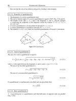
FIG. 3-1

Boundary conditions.

satisfy the differential equation inside the region and the prescribed
conditions on the boundary.
In mathematical language, the propagation problem is known as an
initial-value problem (Fig. 3-2). Schematically, the problem is characterized by a differential equation plus an open region in which the
equation holds. The solution of the differential equation must satisfy
the initial conditions plus any “side” boundary conditions.
The description of phenomena in a “continuous” medium such as a
gas or a fluid often leads to partial differential equations. In particular,
phenomena of “wave” propagation are described by a class of partial
differential equations called “hyperbolic,” and these are essentially
different in their properties from other classes such as those that
describe equilibrium (“elliptic”) or diffusion and heat transfer (“parabolic”). Prototypes are:
1. Elliptic. Laplace’s equation
∂2u ∂2u
ᎏ2 + ᎏ2 = 0
∂x
∂y
Poisson’s equation
∂2u ∂2u

ᎏ2 + ᎏ2 = g(x,y)
∂x
∂y
These do not contain the variable t (time) explicitly; accordingly, their
solutions represent equilibrium configurations. Laplace’s equation
corresponds to a “natural” equilibrium, while Poisson’s equation corresponds to an equilibrium under the influence of g(x, y). Steady heattransfer and mass-transfer problems are elliptic.
2. Parabolic. The heat equation
∂u ∂2u ∂2u
ᎏ = ᎏ2 + ᎏ2
∂t
∂x
∂y
describes unsteady or propagation states of diffusion as well as heat
transfer.
3. Hyperbolic. The wave equation
∂2u ∂2u ∂2u
= ᎏ2 + ᎏ2
ᎏ
∂t2
∂x
∂y
describes wave propagation of all types when the assumption is made
that the wave amplitude is small and that interactions are linear.

where x ϭ mass, energy, etc. These statements may be abbreviated by
the statement
Input − output + production = accumulation
Many general laws of the physical universe are expressible by differential equations. Specific phenomena are then singled out from the
infinity of solutions of these equations by assigning the individual initial or boundary conditions which characterize the given problem. For
steady state or boundary-value problems (Fig. 3-1) the solution must


FIG. 3-2

Propagation problem.
3-3


3-4

MATHEMATICS

The solution phase has been characterized in the past by a concentration on methods to obtain analytic solutions to the mathematical
equations. These efforts have been most fruitful in the area of the linear equations such as those just given. However, many natural phenomena are nonlinear. While there are a few nonlinear problems that
can be solved analytically, most cannot. In those cases, numerical
methods are used. Due to the widespread availability of software for
computers, the engineer has quite good tools available.
Numerical methods almost never fail to provide an answer to any
particular situation, but they can never furnish a general solution of
any problem.
The mathematical details outlined here include both analytic and
numerical techniques useful in obtaining solutions to problems.
Our discussion to this point has been confined to those areas in which
the governing laws are well known. However, in many areas, information on the governing laws is lacking and statistical methods are reused.
Broadly speaking, statistical methods may be of use whenever conclusions are to be drawn or decisions made on the basis of experimental
evidence. Since statistics could be defined as the technology of the scientific method, it is primarily concerned with the first two aspects of the
method, namely, the performance of experiments and the drawing of
conclusions from experiments. Traditionally the field is divided into two
areas:
1. Design of experiments. When conclusions are to be drawn or
decisions made on the basis of experimental evidence, statistical techniques are most useful when experimental data are subject to errors.

The design of experiments may then often be carried out in such a
fashion as to avoid some of the sources of experimental error and
make the necessary allowances for that portion which is unavoidable.
Second, the results can be presented in terms of probability statements which express the reliability of the results. Third, a statistical
approach frequently forces a more thorough evaluation of the experimental aims and leads to a more definitive experiment than would
otherwise have been performed.
2. Statistical inference. The broad problem of statistical inference is to provide measures of the uncertainty of conclusions drawn
from experimental data. This area uses the theory of probability,
enabling scientists to assess the reliability of their conclusions in terms
of probability statements.
Both of these areas, the mathematical and the statistical, are intimately intertwined when applied to any given situation. The methods
of one are often combined with the other. And both in order to be successfully used must result in the numerical answer to a problem—that
is, they constitute the means to an end. Increasingly the numerical
answer is being obtained from the mathematics with the aid of computers. The mathematical notation is given in Table 3-1.
MISCELLANEOUS MATHEMATICAL CONSTANTS
Numerical values of the constants that follow are approximate to the
number of significant digits given.
π = 3.1415926536
e = 2.7182818285
γ = 0.5772156649
ln π = 1.1447298858
log π = 0.4971498727
Radian = 57.2957795131°
Degree = 0.0174532925 rad
Minute = 0.0002908882 rad
Second = 0.0000048481 rad

΂ Α ᎏm − ln n΃ = 0.577215
n


γ = lim

n→∞

Pi
Napierian (natural) logarithm base
Euler’s constant
Napierian (natural) logarithm of pi, base e
Briggsian (common logarithm of pi, base 10

1

TABLE 3-1

Mathematical Signs, Symbols, and Abbreviations

Ϯ (ϯ)
:
ϻ
<
Ͽ
>
Ѐ
Х
∼
Ё
≠
Џ
∝
∞

∴
͙ෆෆ
3
ෆෆ
͙
n
͙ෆෆ
Є
⊥
ʈ
|x|
log or log10
loge or ln
e
a°
a′ a
a″ a
sin
cos
tan
ctn or cot
sec
csc
vers
covers
exsec
sin−1
sinh
cosh
tanh

sinh−1
f(x) or φ(x)
∆x
Α
dx
dy/dx or y′
d2y/dx2 or y″
dny/dxn
∂y/∂x
∂ny/∂xn
∂nz
ᎏ
∂x∂y

Ύ

͵

The natural numbers, or counting numbers, are the positive integers:
1, 2, 3, 4, 5, . . . . The negative integers are −1, −2, −3, . . . .
A number in the form a/b, where a and b are integers, b ≠ 0, is a
rational number. A real number that cannot be written as the quotient
of two
integers is called an irrational number, e.g., ͙ෆ2, ͙ෆ3, ͙ෆ5, π,
3
e, ͙ෆ2.

nth partial derivative with respect to x and y
integral of


b

integral between the limits a and b

a

y˙
y¨
∆ or ∇2

first derivative of y with respect to time
second derivative of y with respect to time
the “Laplacian”
∂2
∂2
∂2
ᎏ2 + ᎏ2 + ᎏ2
∂x
∂y
∂z
sign of a variation
sign for integration around a closed path

΂

m=1

THE REAL-NUMBER SYSTEM

plus or minus (minus or plus)

divided by, ratio sign
proportional sign
less than
not less than
greater than
not greater than
approximately equals, congruent
similar to
equivalent to
not equal to
approaches, is approximately equal to
varies as
infinity
therefore
square root
cube root
nth root
angle
perpendicular to
parallel to
numerical value of x
common logarithm or Briggsian logarithm
natural logarithm or hyperbolic logarithm or Naperian
logarithm
base (2.718) of natural system of logarithms
an angle a degrees
prime, an angle a minutes
double prime, an angle a seconds, a second
sine
cosine

tangent
cotangent
secant
cosecant
versed sine
coversed sine
exsecant
anti sine or angle whose sine is
hyperbolic sine
hyperbolic cosine
hyperbolic tangent
anti hyperbolic sine or angle whose hyperbolic sine is
function of x
increment of x
summation of
differential of x
derivative of y with respect to x
second derivative of y with respect to x
nth derivative of y with respect to x
partial derivative of y with respect to x
nth partial derivative of y with respect to x

δ

Ͷ

΃


MATHEMATICS

There is a one-to-one correspondence between the set of real numbers and the set of points on an infinite line (coordinate line).
Order among Real Numbers; Inequalities
a > b means that a − b is a positive real number.
If a < b and b < c, then a < c.
If a < b, then a Ϯ c < b Ϯ c for any real number c.
If a < b and c > 0, then ac < bc.
If a < b and c < 0, then ac > bc.
If a < b and c < d, then a + c < b + d.
If 0 < a < b and 0 < c < d, then ac < bd.
If a < b and ab > 0, then 1/a > 1/b.
If a < b and ab < 0, then 1/a < 1/b.
Absolute Value For any real number x, |x| = x
−x

Ά

a < 0, and n odd, it is the unique negative root, and (3) if a < 0 and n
even, it is any of the complex roots. In cases (1) and (2), the root can
be found on a calculator by taking y = ln a/n and then x = e y. In case
(3), see the section on complex variables.
ALGEBRAIC INEQUALITIES
Arithmetic-Geometric Inequality Let An and Gn denote respectively the arithmetic and the geometric means of a set of positive numbers a1, a2, . . . , an. The An ≥ Gn, i.e.,
a1 + a2 + ⋅ ⋅ ⋅ + an
ᎏᎏ
n

if x ≥ 0
if x < 0

Properties

If |x| = a, where a > 0, then x = a or x = −a.
|x| = |−x|; −|x| ≤ x ≤ |x|; |xy| = |x| |y|.
If |x| < c, then −c < x < c, where c > 0.
||x| − |y|| ≤ |x + y| ≤ |x| + |y|.
͙xෆ2 = |x|.
a = c , then a + b = c + d , a − b = c − d ,
Proportions If ᎏ
ᎏ
ᎏ ᎏ ᎏ ᎏ
b
d
d
b d
b
a−b c−d
ᎏ = ᎏ.
a+b c+d

Form

Example

(∞)(0)
00
∞0
1∞

xe−x
xx
(tan x)cos x

(1 + x)1/x

x→∞
x → 0+
−
x→aπ
x → 0+

∞−∞
0
ᎏ
0
∞
ᎏ
∞

ෆෆ1 − ͙xෆ−
ෆෆ1
͙xෆ+
sin x
ᎏ
x
ex
ᎏ
x

x→∞
x→0
x→∞


n

Α (a a

1 2

⋅ ⋅ ⋅ ar)1/r ≤ neAn

r=1

where e is the best possible constant in this inequality.
Cauchy-Schwarz Inequality Let a = (a1, a2, . . . , an), b = (b1,
b2, . . . , bn), where the ai’s and bi’s are real or complex numbers. Then

Έ Α a bෆ Έ ≤ ΂ Α |a | ΃΂ Α |b | ΃
2

n

n

a−n = 1/an

a≠0

(ab)n = anbn
(an)m = anm,
n

anam = an + m


͙ෆ
a=a
if a > 0
mn
m n
ෆaෆෆ = ͙aෆ, a > 0
͙͙
1/n

n

am a > 0
am/n = (am)1/n = ͙ෆ,
a0 = 1 (a ≠ 0)
0a = 0 (a ≠ 0)
Logarithms log ab = log a + log b, a > 0, b > 0
log an = n log a
log (a/b)
= log a − log b
n
log ͙ aෆ = (1/n) log a
The common logarithm (base 10) is denoted log a or log10 a. The natural logarithm (base e) is denoted ln a (or in some texts log e a). If the
text is ambiguous (perhaps using log x for ln x), test the formula by
evaluating it.
Roots If a is a real number, n is a positive integer, then x is called
the nth root of a if xn = a. The number of nth roots is n, but not all of
them are necessarily real. The principal nth root means the following:
(1) if a > 0 the principal nth root is the unique positive root, (2) if


n

k k

k

2

k

k=1

2

k=1

The equality holds if, and only if, the vectors a, b are linearly dependent (i.e., one vector is scalar times the other vector).
Minkowski’s Inequality Let a1, a2, . . . , an and b1, b2, . . . , bn
be any two sets of complex numbers. Then for any real number
p > 1,

΂ Α |a + b | ΃ ≤ ΂ Α |a | ΃ + ΂ Α |b | ΃
1/p

n

k

k


1/p

n

p

k

k=1

1/p

n

p

k

k=1

p

k=1

Hölder’s Inequality Let a1, a2, . . . , an and b1, b2, . . . , bn be any
two sets of complex numbers, and let p and q be positive numbers
with 1/p + 1/q = 1. Then

Έ Α a bෆ Έ ≤ ΂ Α |a | ΃ ΂ Α |b | ΃
n


1/p

n

k k

Integral Exponents (Powers and Roots) If m and n are positive integers and a, b are numbers or functions, then the following
properties hold:

≥ (a1a2 ⋅ ⋅ ⋅ an)1/n

The equality holds only if all of the numbers ai are equal.
Carleman’s Inequality The arithmetic and geometric means
just defined satisfy the inequality

k=1

Indeterminants

3-5

k

k=1

k=1

1/q


n

p

q

k

k=1

The equality holds if, and only if, the sequences |a1|p, |a2|p, . . . , |an|p
and |b1|q, |b2|q, . . . , |bn|q are proportional and the argument (angle) of
the complex numbers akb
ෆk is independent of k. This last condition is of
course automatically satisfied if a1, . . . , an and b1, . . . , bn are positive
numbers.
Lagrange’s Inequality Let a1, a2, . . . , an and b1, b2, . . . , bn be
real numbers. Then

΂ Α a b ΃ = ΂ Α a ΃΂ Α b ΃ −
2

n

n

k=1

n


2
k

k k

k=1

2
k

k=1

Α

(akbj − aj bk)2

1≤k≤j≤n

Example Two chemical engineers, John and Mary, purchase stock in the
same company at times t1, t2, . . . , tn, when the price per share is respectively p1,
p2, . . . , pn. Their methods of investment are different, however: John purchases
x shares each time, whereas Mary invests P dollars each time (fractional shares
can be purchased). Who is doing better?
While one can argue intuitively that the average cost per share for Mary does
not exceed that for John, we illustrate a mathematical proof using inequalities.
The average cost per share for John is equal to
n

x Α pi


1 n
Total money invested
i=1
ᎏᎏᎏᎏ = ᎏ = ᎏ Α pi
nx
Number of shares purchased
n i=1
The average cost per share for Mary is
nP
n
ᎏ
=ᎏ
n
n
P
1
ᎏᎏ
Α ᎏᎏ iΑ
i = 1 pi
= 1 pi


3-6

MATHEMATICS

Thus the average cost per share for John is the arithmetic mean of p1, p2, . . . , pn,
whereas that for Mary is the harmonic mean of these n numbers. Since the harmonic mean is less than or equal to the arithmetic mean for any set of positive
numbers and the two means are equal only if p1 = p2 = ⋅⋅⋅ = pn, we conclude that
the average cost per share for Mary is less than that for John if two of the prices

pi are distinct. One can also give a proof based on the Cauchy-Schwarz inequality. To this end, define the vectors
a = (p1−1/2, p2−1/2, . . . , pn−1/2)

Then a ⋅ b = 1 + ⋅⋅⋅ + 1 = n, and so by the Cauchy-Schwarz inequality
n
1
(a ⋅ b)2 = n2 ≤ Α ᎏ
i = 1 pi

n

Αp

i

i=1

with the equality holding only if p1 = p2 = ⋅⋅⋅ = pn. Therefore
n

Αp

i

b = (p11/2, p21/2, . . . , pn1/2)

i=1
n
ᎏ
ᎏ

n
1 ≤ n
Α ᎏᎏ
i = 1 pi

MENSURATION FORMULAS
REFERENCES: Liu, J., Mathematical Handbook of Formulas and Tables,
McGraw-Hill, New York (1999); />html, etc.

Area of Regular Polygon of n Sides Inscribed in a Circle of
Radius r
A = (nr 2/2) sin (360°/n)

Let A denote areas and V volumes in the following.

Perimeter of Inscribed Regular Polygon

PLANE GEOMETRIC FIGURES WITH
STRAIGHT BOUNDARIES

P = 2nr sin (180°/n)

Triangles (see also “Plane Trigonometry”) A = a bh where b =
base, h = altitude.
Rectangle A = ab where a and b are the lengths of the sides.
Parallelogram (opposite sides parallel) A = ah = ab sin α where
a, b are the lengths of the sides, h the height, and α the angle between
the sides. See Fig. 3-3.
Rhombus (equilateral parallelogram) A = aab where a, b are the
lengths of the diagonals.

Trapezoid (four sides, two parallel) A = a(a + b)h where the
lengths of the parallel sides are a and b, and h = height.
Quadrilateral (four-sided) A = aab sin θ where a, b are the
lengths of the diagonals and the acute angle between them is θ.
Regular Polygon of n Sides See Fig. 3-4.
180°
1
A = ᎏ nl 2 cot ᎏ
where l = length of each side
n
4
180°
l
R = ᎏ csc ᎏ
where R is the radius of the circumscribed circle
n
2
180°
l
r = ᎏ cot ᎏ
where r is the radius of the inscribed circle
n
2
Radius r of Circle Inscribed in Triangle with Sides a, b, c
r=

ᎏᎏ
Ί๶๶
s
(s − a)(s − b)(s − c)


where s = a(a + b + c)

Radius R of Circumscribed Circle
abc
R = ᎏᎏᎏ
4͙ෆ
s(ෆ
sෆ
−ෆaෆ
)(ෆ
sෆ
−ෆ
bෆ
)(ෆ
sෆ
−ෆcෆ)

FIG. 3-3

Parallelogram.

FIG. 3-4

Regular polygon.

Area of Regular Polygon Circumscribed about a Circle of
Radius r
A = nr 2 tan (180°/n)
Perimeter of Circumscribed Regular Polygon

180°
P = 2nr tan ᎏ
n
PLANE GEOMETRIC FIGURES
WITH CURVED BOUNDARIES
Circle (Fig. 3-5) Let
C = circumference
r = radius
D = diameter
A = area
S = arc length subtended by θ
l = chord length subtended by θ
H = maximum rise of arc above chord, r − H = d
θ = central angle (rad) subtended by arc S
C = 2πr = πD
(π = 3.14159 . . .)
S = rθ = aDθ
l = 2͙ෆ
r2ෆ
−ෆ
dෆ2 = 2r sin (θ/2) = 2d tan (θ/2)
θ
1
1
d = ᎏ ͙ෆ4ෆ
r2ෆ
−ෆl2ෆ = ᎏ l cot ᎏ
2
2
2

S
d
l
θ = ᎏ = 2 cos−1 ᎏ = 2 sin−1 ᎏ
r
r
D

FIG. 3-5

Circle.


MENSURATION FORMULAS

3-7

Frustum of Pyramid (formed from the pyramid by cutting off
the top with a plane

ෆ1ෆ⋅ෆA
ෆ2ෆ)h
V = s (A1 + A2 + ͙A
where h = altitude and A1, A2 are the areas of the base; lateral area of
a regular figure = a (sum of the perimeters of base) × (slant height).
FIG. 3-6

Ellipse.

Volume and Surface Area of Regular Polyhedra with Edge l

FIG. 3-7

Parabola.

A (circle) = πr = dπD
A (sector) = arS = ar 2θ
A (segment) = A (sector) − A (triangle) = ar 2(θ − sin θ)
2

2

Ring (area between two circles of radii r1 and r2 ) The circles need
not be concentric, but one of the circles must enclose the other.
A = π(r1 + r2)(r1 − r2)
Ellipse (Fig. 3-6)

r1 > r2

Let the semiaxes of the ellipse be a and b
A = πab
C = 4aE(e)

where e2 = 1 − b2/a2 and E(e) is the complete elliptic integral of the
second kind,
π
1 2
E(e) = ᎏ 1 − ᎏ e2 + ⋅ ⋅ ⋅
2
2


΄ ΂΃

΅

ෆ2ෆ+
ෆෆb2ෆ)/2
ෆ].
[an approximation for the circumference C = 2π ͙(a
Parabola (Fig. 3-7)
2
2x + ͙ෆ4ෆ
xෆ
+ෆy2ෆ
y2
Length of arc EFG = ͙ෆ4ෆ
x2ෆ
+ෆy2ෆ + ᎏ ln ᎏᎏ
y
2x
4
Area of section EFG = ᎏ xy
3
Catenary (the curve formed by a cord of uniform weight suspended freely between two points A, B; Fig. 3-8)
y = a cosh (x/a)
Length of arc between points A and B is equal to 2a sinh (L/a). Sag of
the cord is D = a cosh (L/a) − a.
SOLID GEOMETRIC FIGURES WITH PLANE BOUNDARIES
Cube Volume = a3; total surface area = 6a2; diagonal = a͙3ෆ,
where a = length of one side of the cube.
Rectangular Parallelepiped Volume = abc; surface area =

2
ෆ
2(ab + ac + bc); diagonal = ͙ෆ
a2ෆ
+ෆ
bෆ
+ෆc2ෆ, where a, b, c are the lengths
of the sides.
Prism Volume = (area of base) × (altitude); lateral surface area =
(perimeter of right section) × (lateral edge).
Pyramid Volume = s (area of base) × (altitude); lateral area of
regular pyramid = a (perimeter of base) × (slant height) = a (number
of sides) (length of one side) (slant height).

FIG. 3-8

Catenary.

Type of surface

Name

Volume

Surface area

4 equilateral triangles
6 squares
8 equilateral triangles
12 pentagons

20 equilateral triangles

Tetrahedron
Hexahedron (cube)
Octahedron
Dodecahedron
Icosahedron

0.1179 l3
1.0000 l3
0.4714 l3
7.6631 l3
2.1817 l3

1.7321 l2
6.0000 l2
3.4641 l2
20.6458 l2
8.6603 l2

SOLIDS BOUNDED BY CURVED SURFACES
Cylinders (Fig. 3-9) V = (area of base) × (altitude); lateral surface
area = (perimeter of right section) × (lateral edge).
Right Circular Cylinder V = π (radius)2 × (altitude); lateral surface area = 2π (radius) × (altitude).
Truncated Right Circular Cylinder
V = πr 2h; lateral area = 2πrh
h = a (h1 + h2)
Hollow Cylinders Volume = πh(R2 − r 2), where r and R are the
internal and external radii and h is the height of the cylinder.
Sphere (Fig. 3-10)

V (sphere) = 4⁄ 3πR3, jπD3
V (spherical sector) = wπR2hi = 2 (open spherical sector), i ϭ1
(spherical cone)
V (spherical segment of one base) = jπh1(3r 22 + h12)
V (spherical segment of two bases) = jπh 2(3r 12 + 3r 22 + h 22 )
A (sphere) = 4πR2 = πD2
A (zone) = 2πRh = πDh
A (lune on the surface included between two great circles, the inclination of which is θ radians) = 2R2θ.
Cone V = s (area of base) × (altitude).
Right Circular Cone V = (π/3) r 2h, where h is the altitude and r
is the radius of the base; curved surface area = πr ͙ෆ
r2ෆ
+ෆ
h2ෆ, curved sur2
face of the frustum of a right cone = π(r1 + r2) ͙ෆ
h2ෆෆ
+ෆ(ෆ
r1ෆ
−ෆrෆ
2)ෆ, where
r1, r2 are the radii of the base and top, respectively, and h is the altitude; volume of the frustum of a right cone = π(h/3)(r 21 + r1r2 + r 22) =
h/3(A1 + A2 + ͙ෆ
Aෆ
1Aෆ2), where A1 = area of base and A2 = area of top.
Ellipsoid V = (4 ⁄3) πabc, where a, b, c are the lengths of the semiaxes.
Torus (obtained by rotating a circle of radius r about a line whose
distance is R > r from the center of the circle)
V = 2π2Rr 2

FIG. 3-9


Cylinder.

Surface area = 4π2Rr

FIG. 3-10

Sphere.


3-8

MATHEMATICS

Prolate Spheroid (formed by rotating an ellipse about its major
axis [2a])
Surface area = 2πb + 2π(ab/e) sin e

43

1+e
b2
Surface area = 2πa2 + π ᎏ ln ᎏ
e
1−e

b

2


where a, b are the major and minor axes and e = eccentricity (e < 1).
Oblate Spheroid (formed by the rotation of an ellipse about its
minor axis [2b]) Data as given previously.

͵ y ds

S = 2π

V = ⁄ πab

−1

2

Area of a Surface of Revolution
a

ෆyෆ/d
ෆx)
ෆ2ෆ dx and y = f(x) is the equation of the plane
where ds = ͙1ෆෆ
+ෆ(d
curve rotated about the x axis to generate the surface.
Area Bounded by f(x), the x Axis, and the Lines x = a, x = b

͵ f(x) dx
b

A=


V = 4 ⁄3πa2b

For process vessels, the formulas reduce to the following:
Hemisphere
␲
␲
V = ᎏᎏ D3, A = ᎏᎏ D2
12
2
For a hemisphere (concave up) partially filled to a depth h1, use the
formulas for spherical segment with one base, which simplify to

[ f(x) ≥ 0]

a

Length of Arc of a Plane Curve
If y = f(x),
Length of arc s =

dy
͵ Ί1๶๶+๶๶
΂ᎏ
΃ dx
dx ๶

Length of arc s =

dx
͵ Ί1๶๶+๶๶

΂ᎏ
΃ dy
dy ๶

b

2

a

If x = g(y),
2

d

c

V = ␲h12(RϪh1/3) = ␲h12(D/2 − h1/3)

If x = f(t), y = g(t),

A = 2␲Rh1 ϭ ␲Dh1
For a hemisphere (concave down) partially filled from the bottom, use
the formulas for a spherical segment of two bases, one of which is a
plane through the center, where h = distance from the center plane to
the surface of the partially filled hemisphere.

Length of arc s =

dy

dx
͵ Ί΂๶๶
+ ΂ᎏ๶
dt
ᎏ๶
dt ΃ ๶๶๶
dt ΃
t1

2

2

t0

In general, (ds)2 = (dx)2 + (dy)2.

V = ␲h(R2Ϫh2/3) = ␲h(D2/4 − h2/3)

IRREGULAR AREAS AND VOLUMES

A = 2␲Rh = ␲Dh

Irregular Areas Let y0, y1, . . . , yn be the lengths of a series of
equally spaced parallel chords and h be their distance apart (Fig. 3-11).
The area of the figure is given approximately by any of the following:

Cone For a cone partially filled, use the same formulas as for
right circular cones, but use r and h for the region filled.
Ellipsoid If the base of a vessel is one-half of an oblate spheroid

(the cross section fitting to a cylinder is a circle with radius of D/2 and
the minor axis is smaller), then use the formulas for one-half of an
oblate spheroid.
V ϭ 0.1745D3, S ϭ 1.236D2, minor axis ϭ D/3
V ϭ 0.1309D , S ϭ 1.084D , minor axis ϭ D/4
3

2

AT = (h/2)[(y0 + yn) + 2(y1 + y2 + ⋅ ⋅ ⋅ + yn − 1)]

(trapezoidal rule)

As = (h/3)[(y0 + yn) + 4(y1 + y3 + y5 + ⋅ ⋅ ⋅ + yn − 1)
+ 2(y2 + y4 + ⋅ ⋅ ⋅ + yn − 2)]

(n even, Simpson’s rule)

The greater the value of n, the greater the accuracy of approximation.
Irregular Volumes To find the volume, replace the y’s by crosssectional areas Aj and use the results in the preceding equations.

MISCELLANEOUS FORMULAS
See also “Differential and Integral Calculus.”
Volume of a Solid Revolution (the solid generated by rotating
a plane area about the x axis)

͵ [ f(x)] dx
b

V=π


2

a

where y = f(x) is the equation of the plane curve and a ≤ x ≤ b.

FIG. 3-11

Irregular area.

ELEMENTARY ALGEBRA
REFERENCES: Stillwell, J. C., Elements of Algebra, CRC Press, New York
(1994); Rich, B., and P. Schmidt, Schaum's Outline of Elementary Algebra,
McGraw-Hill, New York (2004).

OPERATIONS ON ALGEBRAIC EXPRESSIONS
An algebraic expression will here be denoted as a combination of letters and numbers such as
3ax − 3xy + 7x2 + 7x 3/ 2 − 2.8xy
Addition and Subtraction Only like terms can be added or subtracted in two algebraic expressions.

Example (3x + 4xy − x2) + (3x2 + 2x − 8xy) = 5x − 4xy + 2x2.
Example (2x + 3xy − 4x1/2) + (3x + 6x − 8xy) = 2x + 3x + 6x − 5xy − 4x1/2.
Multiplication Multiplication of algebraic expressions is term by
term, and corresponding terms are combined.
Example (2x + 3y − 2xy)(3 + 3y) = 6x + 9y + 9y2 − 6xy2.
Division This operation is analogous to that in arithmetic.
Example Divide 3e2x + ex + 1 by ex + 1.



ELEMENTARY ALGEBRA
PROGRESSIONS

Dividend
Divisor ex + 1 | 3e2x + ex + 1 3ex − 2 quotient
3e2x + 3ex

An arithmetic progression is a succession of terms such that each
term, except the first, is derivable from the preceding by the addition
of a quantity d called the common difference. All arithmetic progressions have the form a, a + d, a + 2d, a + 3d, . . . . With a = first term,
l = last term, d = common difference, n = number of terms, and s =
sum of the terms, the following relations hold:

−2e + 1
−2ex − 2
x

+ 3 (remainder)
Therefore, 3e + e + 1 = (e + 1)(3e − 2) + 3.
2x

x

x

x

s (n − 1)
l = a + (n − 1)d = ᎏ + ᎏ d
2

n

Operations with Zero All numerical computations (except division) can be done with zero: a + 0 = 0 + a = a; a − 0 = a; 0 − a = −a;
(a)(0) = 0; a0 = 1 if a ≠ 0; 0/a = 0, a ≠ 0. a/0 and 0/0 have no meaning.
Fractional Operations
−x
x
−x
x −x
x ax
x
− ᎏ = − ᎏ = ᎏ = ᎏ ; ᎏ = ᎏ ; ᎏ = ᎏ , if a ≠ 0.
y
y
−y
−y
y −y
y ay

n
n
n
s = ᎏ [2a + (n − 1)d] = ᎏ (a + l) = ᎏ [2l − (n − 1)d]
2
2
2

΂ ΃

΂ᎏy ΃΂ᎏt ΃ = ᎏyt ;


x
z xϮz
ᎏ Ϯ ᎏ = ᎏᎏ;
y
y
y

x

z

xz

s (n − 1)d 2s
a = l − (n − 1)d = ᎏ − ᎏ = ᎏ − l
2
n
n

΂ ΃΂ ΃

xt
x/y
x t
ᎏ= ᎏ ᎏ =ᎏ
z/t
y z
yz


l−a
2(s − an) 2(nl − s)
d=ᎏ=ᎏ=ᎏ
n−1
n(n − 1)
n(n − 1)

Factoring That process of analysis consisting of reducing a given
expression into the product of two or more simpler expressions called
factors. Some of the more common expressions are factored here:
(2) x + 2xy + y = (x + y)
2

l−a
2s
n=ᎏ+1=ᎏ
d
l+a
The arithmetic mean or average of two numbers a, b is (a + b)/2;
of n numbers a1, . . . , an is (a1 + a2 + ⋅ ⋅ ⋅ + an)/n.
A geometric progression is a succession of terms such that each
term, except the first, is derivable from the preceding by the multiplication of a quantity r called the common ratio. All such progressions
have the form a, ar, ar 2, . . . , ar n − 1. With a = first term, l = last term,
r = ratio, n = number of terms, s = sum of the terms, the following relations hold:
[a + (r − 1)s] (r − 1)sr n − 1
l = ar n − 1 = ᎏᎏ = ᎏᎏ
r
rn − 1

(1) (x2 − y2) = (x − y)(x + y)

2

2

(3) x3 − y3 = (x − y)(x2 + xy + y2)
(4) (x3 + y3) = (x + y)(x2 − xy + y2)
(5) (x4 − y4) = (x − y)(x + y)(x2 + y2)
(6) x5 + y5 = (x + y)(x4 − x3y + x2y2 − xy3 + y4)
(7) xn − yn = (x − y)(xn − 1 + xn − 2y + xn − 3y2 + ⋅ ⋅ ⋅ + yn − 1)
Laws of Exponents
(an)m = anm; an + m = an ⋅ am; an/m = (an)1/m; an − m = an/am; a1/m = m͙aෆ;
a1/2 = ͙ෆa; ͙ෆ
x2 = |x| (absolute value of x). For x > 0, y > 0, ͙xy
ෆ = ͙xෆ
n
n
n
͙ෆ
y; for x > 0 ͙ෆ
xm = xm/n; ͙ෆ
1ෆ
/x = 1/͙xෆ

a(r n − 1) a(1 − r n) rl − a
lr n − l
s=ᎏ=ᎏ=ᎏ=ᎏ
r−1
1−r
r − 1 rn − rn − 1
log l − log a

l
(r − 1)s
s−a
a=ᎏ
=ᎏ
, r = ᎏ , log r = ᎏᎏ
rn − l
rn − 1
s−l
n−1
log l − log a
log[a + (r − 1)s] − log a
n = ᎏᎏ + 1 = ᎏᎏᎏ
log r
log r

THE BINOMIAL THEOREM
If n is a positive integer,

ෆ; of n
The geometric mean of two nonnegative numbers a, b is ͙ab
numbers is (a1a2 . . . an)1/n. The geometric mean of a set of positive
numbers is less than or equal to the arithmetic mean.

n(n − 1)
(a + b)n = an + nan − 1b + ᎏ an − 2 b2
2!
n
n(n − 1)(n − 2)
n n−j j

+ ᎏᎏ an − 3b3 + ⋅ ⋅ ⋅ + bn = Α
a b
j
3!
j=0

΂΃

΂΃

n
n!
where
= ᎏ = number of combinations of n things taken j at
j
j!(n − j)!
a time. n! = 1 ⋅ 2 ⋅ 3 ⋅ 4 ⋅ ⋅ ⋅ n, 0! = 1.
Example Find the sixth term of (x + 2y)12. The sixth term is obtained by
setting j = 5. It is

΂5΃x
12

n

(2y)5 = 792x7(2y)5

Example Find the sum of 1 + a + d + ⋅ ⋅ ⋅ + 1⁄64. Here a = 1, r = a, n = 7.
Thus


a(1⁄64) − 1
s = ᎏᎏ = 127/64
a−1
a
ar n
s = a + ar + ar 2 + ⋅ ⋅ ⋅ + ar n − 1 = ᎏ − ᎏ
1−r 1−r
a
If |r| < 1,
then
lim s = ᎏ
n→∞
1−r
which is called the sum of the infinite geometric progression.

Example The present worth (PW) of a series of cash flows Ck at the end
of year k is

Α ΂ j ΃ = (1 + 1)
14

Example

12 − 5

3-9

14

= 214.


j=0

If n is not a positive integer, the sum formula no longer applies and
an infinite series results for (a + b)n. The coefficients are obtained
from the first formulas in this case.
Example (1 + x)1/2 = 1 + ax − a ⋅ dx2 + a ⋅ d ⋅ 3⁄ 6 x3 ⋅ ⋅ ⋅ (convergent for

x2 < 1).

Additional discussion is under “Infinite Series.”

n
Ck
PW = Α ᎏk
k = 1 (1 + i)
where i is an assumed interest rate. (Thus the present worth always requires
specification of an interest rate.) If all the payments are the same, Ck = R, the
present worth is
n
1
PW = R Α ᎏk
k = 1 (1 + i)

This can be rewritten as
R
PW = ᎏ
1+i

n


Α

k=1

R
1
=ᎏ
ᎏ
(1 + i)k − 1 1 + i

n−1

Α

j=0

1
ᎏj
(1 + i)


3-10

MATHEMATICS

This is a geometric series with r = 1/(1 + i) and a = R/(1 + i). The formulas above
give
R (1 + i)n − 1
PW (=s) = ᎏ ᎏᎏ

(1 + i)n
i
The same formula applies to the value of an annuity (PW) now, to provide for
equal payments R at the end of each of n years, with interest rate i.

A progression of the form a, (a + d )r, (a + 2d)r 2, (a + 3d)r 3, etc., is
a combined arithmetic and geometric progression. The sum of n such
terms is
a − [a + (n − 1)d]r n rd(1 − r n − 1)
s = ᎏᎏ + ᎏᎏ
1−r
(1 − r)2
a
If |r| < 1, lim s = ᎏ + rd/(1 − r)2.
n→∞
1−r
The non-zero numbers a, b, c, etc., form a harmonic progression if
their reciprocals 1/a, 1/b, 1/c, etc., form an arithmetic progression.
Example The progression 1, s, 1⁄5, 1⁄7, . . . , 1⁄31 is harmonic since 1, 3, 5,
7, . . . , 31 form an arithmetic progression.

Cubic Equations A cubic equation, in one variable, has the form
x3 + bx2 + cx + d = 0. Every cubic equation having complex coefficients
has three complex roots. If the coefficients are real numbers, then at
least one of the roots must be real. The cubic equation x3 + bx2 + cx +
d = 0 may be reduced by the substitution x = y − (b/3) to the form y3 +
py + q = 0, where p = s(3c − b2), q = 1⁄27(27d − 9bc + 2b3). This equation has the solutions y1 = A + B, y2 = −a(A + B) + (i͙ෆ3/2)(A − B),
3
y3 = −a(A + B) − (i͙ෆ3/2)(A − B), where i2 = −1, A = ͙ෆ
−ෆ

qෆ
/2ෆ
+ෆ
R,
͙ෆ
3
3
2
B = ͙ෆ
−ෆ
qෆ
/2ෆ
−ෆ
R, and R = (p/3) + (q/2) . If b, c, d are all real and if
͙ෆ
R > 0, there are one real root and two conjugate complex roots; if R =
0, there are three real roots, of which at least two are equal; if R < 0,
there are three real unequal roots. If R < 0, these formulas are impractical. In this case, the roots are given by yk = ϯ 2 ͙ෆ
−ෆ
pෆ
/3 cos [(φ/3) +
120k], k = 0, 1, 2 where
φ = cos−1

ability of throwing such that their sum is 7? Seven may arise in 6 ways: 1 and 6,
2 and 5, 3 and 4, 4 and 3, 5 and 2, 6 and 1. The probability of shooting 7 is j.

THEORY OF EQUATIONS
Linear Equations A linear equation is one of the first degree
(i.e., only the first powers of the variables are involved), and the

process of obtaining definite values for the unknown is called solving
the equation. Every linear equation in one variable is written Ax + B =
0 or x = −B/A. Linear equations in n variables have the form
a11 x1 + a12 x2 + ⋅ ⋅ ⋅ + a1n xn = b1
a21 x1 + a22 x2 + ⋅ ⋅ ⋅ + a2n xn = b2
Ӈ
am1 x1 + am2 x2 + ⋅ ⋅ ⋅ + amn xn = bm
The solution of the system may then be found by elimination or matrix
methods if a solution exists (see “Matrix Algebra and Matrix Computations”).
Quadratic Equations Every quadratic equation in one variable
is expressible in the form ax 2 + bx + c = 0. a ≠ 0. This equation has two
solutions, say, x1, x2, given by

ෆෆ4ac
ෆ
x1
b2ෆ−
−b Ϯ ͙ෆ
= ᎏᎏ
x2
2a

·

If a, b, c are real, the discriminant b2 − 4ac gives the character of the
roots. If b2 − 4ac > 0, the roots are real and unequal. If b2 − 4ac < 0, the
roots are complex conjugates. If b2 − 4ac = 0 the roots are real and
equal. Two quadratic equations in two variables can in general be
solved only by numerical methods (see “Numerical Analysis and
Approximate Methods”).


3

Example y3 − 7y + 7 = 0. p = −7, q = 7, R < 0. Hence
28
φ
ᎏ cos ΂ ᎏ + 120k΃
Ί๶
3
3

yk = −

PERMUTATIONS, COMBINATIONS, AND PROBABILITY

Example Two dice may be thrown in 36 separate ways. What is the prob-

2

and the upper sign applies if q > 0, the lower if q < 0.

The harmonic mean of two numbers a, b is 2ab/(a + b).

Each separate arrangement of all or a part of a set of things is called a
permutation. The number of permutations of n things taken r at a
time, written
n!
P(n, r) = ᎏ = n(n − 1)(n − 2) ⋅⋅⋅ (n − r + 1)
(n − r)!
Each separate selection of objects that is possible irrespective of the

order in which they are arranged is called a combination. The number
of combinations of n things taken r at a time, written C(n, r) = n!/
[r!(n − r)!].
An important relation is r! C(n, r) = P(n, r).
If an event can occur in p ways and fail to occur in q ways, all ways
being equally likely, the probability of its occurrence is p/(p + q), and
that of its failure q/(p + q).

q /4
ᎏ
Ί๶
−p /27

where

27 φ
ᎏ , ᎏ = 3.6311315 rad = 3°37′52″
Ί๶
28 3

φ = cos−1

The roots are approximately −3.048917, 1.692021, and 1.356896.

Example Many equations of state involve solving cubic equations for the
compressibility factor Z. For example, the Redlich-Kwong-Soave equation of
state requires solving
Z 3 − Z 2 + cZ + d = 0,

d<0


where c and d depend on critical constants of the chemical species. In this case,
only positive solutions, Z > 0, are desired.

Quartic Equations See Abramowitz and Stegun (1972, p. 17).
General Polynomials of the nth Degree Denote the general
polynomial equation of degree n by
P(x) = a0 x n + a1 x n − 1 + ⋅ ⋅ ⋅ + an − 1 x + an = 0
If n > 4, there is no formula which gives the roots of the general equation. For fourth and higher order (even third order), the roots can be
found numerically (see “Numerical Analysis and Approximate Methods”). However, there are some general theorems that may prove useful.
Remainder Theorems When P(x) is a polynomial and P(x) is
divided by x − a until a remainder independent of x is obtained, this
remainder is equal to P(a).
Example P(x) = 2x4 − 3x2 + 7x − 2 when divided by x + 1 (here a = −1)
results in P(x) = (x + 1)(2x3 − 2x2 − x + 8) − 10 where −10 is the remainder. It is
easy to see that P(−1) = −10.
Factor Theorem If P(a) is zero, the polynomial P(x) has the factor x − a. In other words, if a is a root of P(x) = 0, then x − a is a factor
of P(x).
If a number a is found to be a root of P(x) = 0, the division of P(x) by
(x − a) leaves a polynomial of degree one less than that of the original
equation, i.e., P(x) = Q(x)(x − a). Roots of Q(x) = 0 are clearly roots of
P(x) = 0.
Example P(x) = x3 − 6x2 + 11x − 6 = 0 has the root + 3. Then P(x) =

(x − 3)(x2 − 3x + 2). The roots of x2 − 3x + 2 = 0 are 1 and 2. The roots of P(x) are
therefore 1, 2, 3.

Fundamental Theorem of Algebra Every polynomial of degree
n has exactly n real or complex roots, counting multiplicities.
Every polynomial equation a0 x n + a1 x n − 1 + ⋅⋅⋅ + an = 0 with rational

coefficients may be rewritten as a polynomial, of the same degree, with
integral coefficients by multiplying each coefficient by the least common
multiple of the denominators of the coefficients.
Example The coefficients of 3⁄2 x4 + 7⁄3 x3 − 5⁄6 x2 + 2x − j = 0 are rational
numbers. The least common multiple of the denominators is 2 × 3 = 6. Therefore, the equation is equivalent to 9x4 + 14x3 − 5x2 + 12x − 1 = 0.


ANALYTIC GEOMETRY
Determinants Consider the system of two linear equations
a11x1 + a12x2 = b1
If the first equation is multiplied by a22 and the second by −a12 and the
results added, we obtain
(a11a22 − a21a12)x1 = b1a22 − b2a12
The expression a11a22 − a21a12 may be represented by the symbol
a11 a12
= a11a22 − a21a12
a21 a22
This symbol is called a determinant of second order. The value of the
square array of n2 quantities aij, where i = 1, . . . , n is the row index,
j = 1, . . . , n the column index, written in the form
|A| =

Έ

Έ

Έ

= a31


Έ

a11 a12
a21 a22
Ӈ
an1 an2

a13 ⋅ ⋅ ⋅ a1n
⋅ ⋅ ⋅ ⋅ ⋅ a2n
an3 ⋅ ⋅ ⋅ ann

Έ

Έ

a11 a12 a13
a
a
a21 a22 a23 The minor of a23 is M23 = 11 12
a31 a32
a31 a32 a33

Έ

Έ

The cofactor Aij of the element aij is the signed minor of aij determined
by the rule Aij = (−1) i + jMij. The value of |A| is obtained by forming any of the
n
n

equivalent expressions Α j = 1 aij Aij , Α i = 1 aij Aij, where the elements aij must be
taken from a single row or a single column of A.

Έaa

Έ

Έ

Έ

Έ

a13
a
a
a
a
− a32 11 13 + a33 11 12
a23
a21 a23
a21 a22

12
22

Έ

In general, Aij will be determinants of order n − 1, but they may in turn be
expanded by the rule. Also,


Έ

is called a determinant. The n2 quantities aij are called the elements
of the determinant. In the determinant |A| let the ith row and jth
column be deleted and a new determinant be formed having n − 1
rows and columns. This new determinant is called the minor of aij
denoted Mij.
Example

Example
a11 a12 a13
a21 a22 a23 = a31A31 + a32A32 + a33A33
a31 a32 a33

a21x1 + a22x2 = b2

Έ

3-11

n

Αa

j=1

n

ji


Ά

A jk = Α a ij A jk = |A|
0
j=1

i=k
i≠k

Fundamental Properties of Determinants
1. The value of a determinant |A| is not changed if the rows and
columns are interchanged.
2. If the elements of one row (or one column) of a determinant are
all zero, the value of |A| is zero.
3. If the elements of one row (or column) of a determinant are
multiplied by the same constant factor, the value of the determinant is
multiplied by this factor.
4. If one determinant is obtained from another by interchanging
any two rows (or columns), the value of either is the negative of the
value of the other.
5. If two rows (or columns) of a determinant are identical, the value
of the determinant is zero.
6. If two determinants are identical except for one row (or column), the sum of their values is given by a single determinant
obtained by adding corresponding elements of dissimilar rows (or
columns) and leaving unchanged the remaining elements.
7. The value of a determinant is not changed if one row (or column) is multiplied by a constant and added to another row (or column).

ANALYTIC GEOMETRY
REFERENCES: Fuller, G., Analytic Geometry, 7th ed., Addison Wesley Longman

(1994); Larson, R., R. P. Hostetler, and B. H. Edwards, Calculus with Analytic
Geometry, 7th ed., Houghton Mifflin (2001); Riddle, D. F., Analytic Geometry, 6th
ed., Thompson Learning (1996); Spiegel, M. R., and J. Liu, Mathematical Handbook of Formulas and Tables, 2d ed., McGraw-Hill (1999); Thomas, G. B., Jr., and
R. L. Finney, Calculus and Analytic Geometry, 9th ed., Addison-Wesley (1996).

Analytic geometry uses algebraic equations and methods to study geometric problems. It also permits one to visualize algebraic equations in
terms of geometric curves, which frequently clarifies abstract concepts.
PLANE ANALYTIC GEOMETRY
Coordinate Systems The basic concept of analytic geometry is
the establishment of a one-to-one correspondence between the points
of the plane and number pairs (x, y). This correspondence may be
done in a number of ways. The rectangular or cartesian coordinate
system consists of two straight lines intersecting at right angles (Fig.
3-12). A point is designated by (x, y), where x (the abscissa) is the
distance of the point from the y axis measured parallel to the x axis,

FIG. 3-12

Rectangular coordinates.

positive if to the right, negative to the left. y (ordinate) is the distance
of the point from the x axis, measured parallel to the y axis, positive if
above, negative if below the x axis. The quadrants are labeled 1, 2, 3,
4 in the drawing, the coordinates of points in the various quadrants
having the depicted signs. Another common coordinate system is the
polar coordinate system (Fig. 3-13). In this system the position of a
point is designated by the pair (r, θ), r = ͙ෆ
x2ෆ
+ෆy2ෆ being the distance to
the origin 0(0,0) and θ being the angle the line r makes with the positive x axis (polar axis). To change from polar to rectangular coordinates,

use x = r cos θ and y = r sin θ. To change from rectangular to
x2ෆ
+ෆy2ෆ and θ = tan−1 (y/x) if x ≠ 0; θ = π/2
polar coordinates, use r = ͙ෆ
if x = 0. The distance between two points (x1, y1), (x2, y2) is defined
2
2
by d = ͙ෆ
(x1ෆෆ
−ෆxෆ
+ෆ(ෆy1ෆෆ
−ෆ
yෆ
2)ෆෆ
2)ෆ in rectangular coordinates or by d =
2
2
r 1ෆෆ
+ෆrෆ
−ෆ2ෆ
r1ෆ
r2ෆcෆosෆෆ
(θ1ෆෆ
−ෆ
θෆ
͙ෆ
2ෆ
2) in polar coordinates. Other coordinate
systems are sometimes used. For example, on the surface of a sphere
latitude and longitude prove useful.

The Straight Line (Fig. 3-14) The slope m of a straight line is
the tangent of the inclination angle θ made with the positive x axis. If

FIG. 3-13

Polar coordinates.

FIG. 3-14

Straight line.


3-12

MATHEMATICS

(x1, y1) and (x2, y2) are any two points on the line, slope = m = (y2 −
y1)/(x2 − x1). The slope of a line parallel to the x axis is zero; parallel to
the y axis, it is undefined. Two lines are parallel if and only if they have
the same slope. Two lines are perpendicular if and only if the product
of their slopes is −1 (the exception being that case when the lines are
parallel to the coordinate axes). Every equation of the type Ax + By +
C = 0 represents a straight line, and every straight line has an equation
of this form. A straight line is determined by a variety of conditions:
Given conditions

Geometric Properties of a Curve When the Equation Is
Given The analysis of the properties of an equation is facilitated
by the investigation of the equation by using the following techniques:
1. Points of maximum, minimum, and inflection. These may be

investigated by means of the calculus.
2. Symmetry. Let F(x, y) = 0 be the equation of the curve.

Equation of line

(1)
(2)
(3)
(4)
(5)

Parallel to x axis
Parallel y axis
Point (x1, y1) and slope m
Intercept on y axis (0, b), m
Intercept on x axis (a, 0), m

(6)

Two points (x1, y1), (x2, y2)

(7)

Two intercepts (a, 0), (0, b)

y = constant
x = constant
y − y1 = m(x − x1)
y = mx + b
y = m(x − a)

y2 − y1
y − y1 = ᎏ (x − x1)
x2 − x1
x/a + y/b = 1

The angle β a line with slope m1 makes with a line having slope m2
is given by tan β = (m2 − m1)/(m1m2 + 1). A line is determined if the
length and direction of the perpendicular to it (the normal) from the
origin are given (see Fig. 3-15). Let p = length of the perpendicular
and α the angle that the perpendicular makes with the positive x axis.
The equation of the line is x cos ␣ + y sin ␣ = p. The equation of a line
perpendicular to a given line of slope m and passing through a point
(x1, y1) is y − y1 = −(1/m) (x − x1). The distance from a point (x1, y1) to
a line with equation Ax + By + C = 0 is
|Ax1 + By1 + C|
d = ᎏᎏ
A2ෆෆ
+ෆ
B2ෆ
͙ෆ
Occasionally some nonlinear algebraic equations can be reduced to
linear equations under suitable substitutions or changes of variables.
In other words, certain curves become the graphs of lines if the scales
or coordinate axes are appropriately transformed.
Example Consider y = bxn. B = log b. Taking logarithms log y =
n log x + log b. Let Y = log y, X = log x, B = log b. The equation then has the form
Y = nX + B, which is a linear equation. Consider k = k0 exp (−E/RT), taking logarithms loge k = loge k0 − E/(RT). Let Y = loge k, B = loge k0, and m = −E/R,
X = 1/T, and the result is Y = mX + B. Next consider y = a + bxn. If the substitution t = x n is made, then the graph of y is a straight line versus t.
Asymptotes The limiting position of the tangent to a curve as the
point of contact tends to an infinite distance from the origin is called

an asymptote. If the equation of a given curve can be expanded in a
Laurent power series such that
n
n
b
f(x) = Α ak x k + Α ᎏkk
k=0
k=1 x

Condition on F(x, y)

Symmetry

F(x, y) = F(−x, y)
F(x, y) = F(x, −y)
F(x, y) = F(−x, −y)
F(x, y) = F(y, x)

With respect to y axis
With respect to x axis
With respect to origin
With respect to the line y = x

3. Extent. Only real values of x and y are considered in obtaining
the points (x, y) whose coordinates satisfy the equation. The extent of
them may be limited by the condition that negative numbers do not
have real square roots.
4. Intercepts. Find those points where the curves of the function
cross the coordinate axes.
5. Asymptotes. See preceding discussion.

6. Direction at a point. This may be found from the derivative of
the function at a point. This concept is useful for distinguishing among
a family of similar curves.
Example y2 = (x2 + 1)/(x2 − 1) is symmetric with respect to the x and y axis,
the origin, and the line y = x. It has the vertical asymptotes x = Ϯ1. When x = 0,
y2 = −1; so there are no y intercepts. If y = 0, (x2 + 1)/(x2 − 1) = 0; so there are no
x intercepts. If |x| < 1, y2 is negative; so |x| > 1. From x2 = (y2 + 1)/(y2 − 1), y = Ϯ1
are horizontal asymptotes and |y| > 1. As x → 1+, y → + ∞; as x → + ∞, y → + 1.
The graph is given in Fig. 3-16.
Conic Sections The curves included in this group are obtained
from plane sections of the cone. They include the circle, ellipse,
parabola, hyperbola, and degeneratively the point and straight line. A
conic is the locus of a point whose distance from a fixed point called
the focus is in a constant ratio to its distance from a fixed line, called
the directrix. This ratio is the eccentricity e. If e = 0, the conic is a circle; if 0 < e < 1, the conic is an ellipse; if e = 1, the conic is a parabola;
if e > 1, the conic is a hyperbola. Every conic section is representable
by an equation of second degree. Conversely, every equation of second degree in two variables represents a conic. The general equation
of the second degree is Ax2 + Bxy + Cy2 + Dx + Ey + F = 0. Let ⌬ be
defined as the determinant
2A B
D
⌬= B
2C E
D E
2F
The table characterizes the curve represented by the equation.

Έ

B2 − 4AC < 0


n

and

lim f(x) = Α akxk
x→∞

k=0

n

then the equation of the asymptote is y = Α k = 0 ak x k. If n = 1, then the
asymptote is (in general oblique) a line. In this case, the equation of
the asymptote may be written as
y = mx + b

m = lim f′(x)
x→∞

b = lim [f(x) − xf′(x)]
x→∞

FIG. 3-15

Determination of line.

⌬≠0

A⌬ < 0

A ≠ C, an ellipse
A⌬ < 0
A = C, a circle
A⌬ > 0, no locus

⌬=0

FIG. 3-16

Point

Έ

B2 − 4AC = 0

Parabola
2 parallel lines if Q = D2 + E2 −
4(A + C)F > 0
1 straight line if Q = 0, no locus
if Q < 0

Graph of y2 = (x2 + 1)/(x2 − 1).

B2 − 4AC > 0

Hyperbola

2 intersecting
straight lines



ANALYTIC GEOMETRY

3-13

Some common equations in parametric form are given below.
(1) (x − h)2 + (y − k)2 = a2
(x − h)
(y − k)
(2) ᎏ
+ᎏ
=1
a2
b2
2

2

(3) x2 + y2 = a2

Circle (Fig. 3-23) Parameter is angle θ.

x = h + a cos θ
y = k + a sin θ
x = h + a cos φ
y = k + a sin φ
−at
x=ᎏ
t2ෆ
+ෆ

1
͙ෆ

Ά

Ellipse (Fig. 3-20) Parameter is angle φ.
dy
Circle Parameter is t = ᎏ = slope of tangent at (x, y).
dx

a
y=ᎏ
t2ෆ
+ෆ1
͙ෆ

(4) x2 = y + k

Parabola (Fig. 3-22)

x2
y2
(5) ᎏᎏ2 Ϫ ᎏᎏ2 = 1
a
b

Hyperbola with the origin at the center (Fig. 3-21)

x
(6) y = a cosh ᎏ

a

Ά
Ά

(7) Cycloid

s
x = a sinh−1 ᎏ
a

Catenary (such as hanging cable under gravity) Parameter s = arc length from (0, a)
to (x, y).

y2 = a2 + s2
x = a(φ − sin φ)
y = a(1 − cos φ)

Fig. 3.24

Similarly, x = a cos φ, y = b sin φ are the parametric equations of the
ellipse x2/a2 + y2/b2 = 1 with parameter φ.

Example 3x2 + 4xy − 2y2 + 3x − 2y + 7 = 0.

Έ

6
⌬= 4
3


4
−4
−2

Έ

3
−2 = −596 ≠ 0, B2 − 4AC = 40 > 0
14

SOLID ANALYTIC GEOMETRY

The curve is therefore a hyperbola.

The following tabulation gives the form of the more common equations.
Polar equation

Type of curve

(1) r = a
(2) r = 2a cos θ
(3) r = 2a sin θ
(4) r2 − 2br cos (θ − β) + b2 − a2 = 0

Circle, Fig. 3-17
Circle, Fig. 3-18
Circle, Fig. 3-19
Circle at (b, β), radius a


ke
(5) r = ᎏᎏ
1 − e cos θ

e = 1 parabola, Fig. 3-22
0 < e < 1 ellipse, Fig. 3-20
e > 1 hyperbola, Fig. 3-21

Parametric Equations It is frequently useful to write the equations of a curve in terms of an auxiliary variable called a parameter.
For example, a circle of radius a, center at (0, 0), can be written in
the equivalent form x = a cos φ, y = a sin φ where φ is the parameter.

Coordinate Systems The commonly used coordinate systems
are three in number. Others may be used in specific problems [see
Morse, P. M., and H. Feshbach, Methods of Theoretical Physics, vols.
I and II, McGraw-Hill, New York (1953)]. The rectangular (cartesian) system (Fig. 3-25) consists of mutually orthogonal axes x, y, z. A
triple of numbers (x, y, z) is used to represent each point. The cylindrical coordinate system (r, θ, z; Fig. 3-26) is frequently used to locate
a point in space. These are essentially the polar coordinates (r, θ) coupled with the z coordinate. As before, x = r cos θ, y = r sin θ, z = z and
r2 = x2 + y2, y/x = tan θ. If r is held constant and θ and z are allowed to
vary, the locus of (r, θ, z) is a right circular cylinder of radius r along
the z axis. The locus of r = C is a circle, and θ = constant is a plane containing the z axis and making an angle θ with the xz plane. Cylindrical
coordinates are convenient to use when the problem has an axis of
symmetry.
The spherical coordinate system is convenient if there is a point
of symmetry in the system. This point is taken as the origin and the
coordinates (ρ, φ, θ) illustrated in Fig. 3-27. The relations are x =

FIG. 3-17

Circle center (0,0) r = a.


FIG. 3-18

Circle center (a,0) r = 2a cos θ.

FIG. 3-19

Circle center (0,a) r = 2a sin θ.

FIG. 3-20

Ellipse, 0 < e < 1.

FIG. 3-21

Hyperbola, e > 1.

FIG. 3-22

Parabola, e = 1.


3-14

MATHEMATICS

FIG. 3-23

Circle.


FIG. 3-24

Cycloid.

ρ sin φ cos θ, y = ρ sin φ sin θ, z = ρ cos φ, and r = ρ sin φ. θ = constant
is a plane containing the z axis and making an angle θ with the xz plane.
φ = constant is a cone with vertex at 0. ρ = constant is the surface of a
sphere of radius ρ, center at the origin 0. Every point in the space may
be given spherical coordinates restricted to the ranges 0 ≤ φ ≤ π, ρ ≥ 0,
0 ≤ θ < 2π.
Lines and Planes The distance between two points (x1, y1, z1),
2
2
2
(x2, y2, z2) is d = ͙ෆ
(xෆ
−ෆxෆ
+ෆ(ෆyෆ
−ෆyෆ
+ෆ(ෆ
z1ෆ
−ෆzෆ
1ෆ
2)ෆෆ
1ෆ
2)ෆෆ
2)ෆ. There is nothing in
the geometry of three dimensions quite analogous to the slope of a
line in the plane case. Instead of specifying the direction of a line by
a trigonometric function evaluated for one angle, a trigonometric

function evaluated for three angles is used. The angles α, β, γ that
a line segment makes with the positive x, y, and z axes, respectively,
are called the direction angles of the line, and cos α, cos β,
cos γ are called the direction cosines. Let (x1, y1, z1), (x2, y2, z2) be
on the line. Then cos α = (x2 − x1)/d, cos β = (y2 − y1)/d, cos γ =
(z2 − z1)/d, where d = the distance between the two points. Clearly
cos2 α + cos2 β + cos2 γ = 1. If two lines are specified by the direction
cosines (cos α1, cos β1, cos γ1), (cos α2, cos β2, cos γ2), then the angle θ
between the lines is cos θ = cos α1 cos α2 + cos β1 cos β2 + cos γ1 cos γ2.
Thus the lines are perpendicular if and only if θ = 90° or cos α1
cos α2 + cos β1 cos β2 + cos γ1 cos γ2 = 0. The equation of a line with
direction cosines (cos α, cos β, cos γ) passing through (x1, y1, z1) is
(x − x1)/cos α = (y − y1)/cos β = (z − z1)/cos γ.
The equation of every plane is of the form Ax + By + Cz + D = 0.
The numbers
A
B
C
ᎏᎏ
, ᎏᎏ
, ᎏᎏ
A2ෆෆ
+ෆ
B2ෆෆ
+ෆ
C2ෆ ͙ෆ
A2ෆෆ
+ෆ
B2ෆෆ
+ෆ

C2ෆ ͙ෆ
A2ෆෆ
+ෆ
B2ෆෆ
+ෆ
C2ෆ
͙ෆ
are direction cosines of the normal lines to the plane. The plane
through the point (x1, y1, z1) whose normals have these as direction
cosines is A(x − x1) + B(y − y1) + C(z − z1) = 0.
Example Find the equation of the plane through (1, 5, −2) perpendicular
to the line (x + 9)/7 = (y − 3)/−1 = z/8. The numbers (7, −1, 8) are called direction numbers. They are a constant multiple of the direction cosines. cos α =
7/114, cos β = −1/114, cos γ = 8/114. The plane has the equation 7(x − 1) −
1(y − 5) + 8(z + 2) = 0 or 7x − y + 8z + 14 = 0.

FIG. 3-25

Cartesian coordinates.

The distance from the point (x1, y1, z1) to the plane Ax + By + Cz +
D = 0 is
|Ax + By + Cz + D|

1
1
1
d = ᎏᎏᎏ
2
2
2


ෆෆ+
ෆෆ
ෆෆ
Bෆ+
Cෆ
͙A

Space Curves Space curves are usually specified as the set of
points whose coordinates are given parametrically by a system of
equations x = f(t), y = g(t), z = h(t) in the parameter t.
Example The equation of a straight line in space is (x − x1)/a = (y − y1)/b =
(z − z1)/c. Since all these quantities must be equal (say, to t), we may write x =
x1 + at, y = y1 + bt, z = z1 + ct, which represent the parametric equations of the
line.
FIG. 3-26

Cylindrical coordinates.

Example The equations z = a cos βt, y = a sin βt, z = bt, a, β, b positive
constants, represent a circular helix.

FIG. 3-27

Spherical coordinates.

FIG. 3-28

Parabolic cylinder.



ANALYTIC GEOMETRY

3-15

Surfaces The locus of points (x, y, z) satisfying f(x, y, z) = 0,
broadly speaking, may be interpreted as a surface. The simplest surface is the plane. The next simplest is a cylinder, which is a surface
generated by a straight line moving parallel to a given line and passing
through a given curve.
Example The parabolic cylinder y = x2 (Fig. 3-28) is generated by a
straight line parallel to the z axis passing through y = x2 in the plane z = 0.
A surface whose equation is a quadratic in the variables x, y, and z
is called a quadric surface. Some of the more common such surfaces
are tabulated and pictured in Figs. 3-28 to 3-36.

FIG. 3-29

FIG. 3-30

FIG. 3-31

Elliptic paraboloid.

FIG. 3-33

y2
z2
x2
FIG. 3-32 Cone. ᎏ2 + ᎏ2 + ᎏ2 = 0
b

c
a

y2
x2
ᎏ2 + ᎏ2 + cz = 0
b
a

y2
z2
x2
Ellipsoid. ᎏ2 + ᎏ2 + ᎏ2 = 1 (sphere if a = b = c)
b
c
a
FIG. 3-34

y2
x2
Hyperbolic paraboloid. ᎏ2 − ᎏ2 + cz = 0
b
a

FIG. 3-35

y2
x2
Elliptic cylinder. ᎏ2 + ᎏ2 = 1
b

a

FIG. 3-36

Hyperbolic cylinder.

y2
z2
x2
Hyperboloid of one sheet. ᎏ2 + ᎏ2 − ᎏ2 = 1
b
c
a

y2
z2
x2
Hyperboloid of two sheets. ᎏ2 + ᎏ2 − ᎏ2 = −1
b
c
a

y2
x2
ᎏ2 − ᎏ2 = 1
b
a


3-16


MATHEMATICS

PLANE TRIGONOMETRY
REFERENCES: Gelfand, I. M., and M. Saul, Trigonometry, Birkhäuser, Boston
(2001); Heineman, E. Richard, and J. Dalton Tarwater, Plane Trigonometry, 7th
ed., McGraw-Hill (1993).

ANGLES
An angle is generated by the rotation of a line about a fixed center
from some initial position to some terminal position. If the rotation is
clockwise, the angle is negative; if it is counterclockwise, the angle is
positive. Angle size is unlimited. If α, β are two angles such that α +
β = 90°, they are complementary; they are supplementary if α + β =
180°. Angles are most commonly measured in the sexagesimal system
or by radian measure. In the first system there are 360 degrees in one
complete revolution; one degree = 1⁄90 of a right angle. The degree is
subdivided into 60 minutes; the minute is subdivided into 60 seconds.
In the radian system one radian is the angle at the center of a circle
subtended by an arc whose length is equal to the radius of the circle.
Thus 2␲ rad = 360°; 1 rad = 57.29578°; 1° = 0.01745 rad; 1 min =
0.00029089 rad. The advantage of radian measure is that it is dimensionless. The quadrants are conventionally labeled as Fig. 3-37 shows.

II

I

III

IV


FIG. 3-37

Quadrants.

FIG. 3-38

Triangles.

FIG. 3-39

Graph of y = sin x.

FIG. 3-40

Graph of y = cos x.

FIG. 3-41

Graph of y = tan x.

FUNCTIONS OF CIRCULAR TRIGONOMETRY
The trigonometric functions of angles are the ratios between the various sides of the reference triangles shown in Fig. 3-38 for the various
quadrants. Clearly r = ͙ෆ
x2ෆ
+ෆy2ෆ ≥ 0. The fundamental functions (see
Figs. 3-39, 3-40, 3-41) are
Plane Trigonometry
Sine of θ = sin θ = y/r
Cosine of θ = cos θ = x/r

Tangent of θ = tan θ = y/x

Secant of θ = sec θ = r/x
Cosecant of θ = csc θ = r/y
Cotangent of θ = cot θ = x/y

Values of the Trigonometric Functions for Common Angles
θ°

θ, rad

sin θ

cos θ

tan θ

0
30
45
60
90

0
π/6
π/4
π/3
π/2

0

1/2
͙2ෆ/2
͙3ෆ/2
1

1
͙3ෆ/2
͙2ෆ/2
1/2
0

0
͙3ෆ/3
1
͙3ෆ
+∞

If 90° ≤ θ ≤ 180°, sin θ = sin (180° − θ); cos θ = −cos (180° − θ);
tan θ = −tan (180° − θ). If 180° ≤ θ ≤ 270°, sin θ = −sin (270° − θ);
cos θ = −cos (270° − θ); tan θ = tan (270° − θ). If 270° ≤ θ ≤ 360°,
sin θ = −sin (360° − θ); cos θ = cos (360° − θ); tan θ = −tan (360° − θ).
The reciprocal properties may be used to find the values of the other
functions.
If it is desired to find the angle when a function of it is given, the
procedure is as follows: There will in general be two angles between
0° and 360° corresponding to the given value of the function.
Given (a > 0)

Find an acute
angle θ0 such that


Required angles are

sin θ = +a
cos θ = +a
tan θ = +a
sin θ = −a
cos θ = −a
tan θ = −a

sin θ0 = a
cos θ0 = a
tan θ0 = a
sin θ0 = a
cos θ0 = a
tan θ0 = a

θ0 and (180° − θ0)
θ0 and (360° − θ0)
θ0 and (180° + θ0)
180° + θ0 and 360° − θ0
180° − θ0 and 180° + θ0
180° − θ0 and 360° − θ0

Relations between Functions of a Single Angle sec θ = 1/
cos θ; csc θ = 1/sin θ, tan θ = sin θ/cos θ = sec θ/csc θ = 1/cot θ; sin2 θ +
cos2 θ = 1; 1 + tan2 θ = sec2 θ; 1 + cot2 θ = csc2 θ. For 0 ≤ θ ≤ 90° the
following results hold:
θ
θ

sin θ = 2 sin ᎏ cos ᎏ
2
2

΂΃ ΂΃


PLANE TRIGONOMETRY

3-17

θ
θ
cos θ = cos2 ᎏ − sin2 ᎏ
2
2
The cofunction property is very important. cos θ = sin (90° − θ),
sin θ = cos (90° − θ), tan θ = cot (90° − θ), cot θ = tan (90° − θ), etc.
Functions of Negative Angles sin (−θ) = −sin θ, cos (−θ) =
cos θ, tan (−θ) = −tan θ, sec (−θ) = sec θ, csc (−θ) = −csc θ, cot (−θ) =
−cot θ.

΂΃

and

΂΃

FIG. 3-42


Identities
Sum and Difference Formulas Let x, y be two angles. sin (x Ϯ y) =
sin x cos y Ϯ cos x sin y; cos (x Ϯ y) = cos x cos y ϯ sin x sin y; tan
(x Ϯ y) = (tan x Ϯ tan y)/(1 ϯ tan x tan y); sin x Ϯ sin y = 2 sin a(x Ϯ
y) cos a(x ϯ y); cos x + cos y = 2 cos a(x + y) cos a(x − y); cos x − cos
y = −2 sin a(x + y) sin a(x − y); tan x Ϯ tan y = [sin (x Ϯ y)]/(cos x cos
y); sin2 x − sin2 y = cos2 y − cos2 x = sin (x + y) sin (x − y); cos2 x − sin2 y =
cos2 y − sin2 x = cos (x + y) cos (x − y); sin (45° + x) = cos (45° − x);
sin (45° − x) = cos (45° + x); tan (45° Ϯ x) = cot (45° ϯ x).
Multiple and Half Angle Identities Let x = angle, sin 2x = 2 sin x
cos x; sin x = 2 sin ax cos ax; cos 2x = cos2 x − sin2x = 1 − 2 sin2x =
2 cos2x − 1. tan 2x = (2 tan x)/(1 − tan2 x); sin 3x = 3 sin x − 4 sin3x;
cos 3x = 4 cos3 x − 3 cos x. tan 3x = (3 tan x − tan3 x)/(1 − 3 tan2 x);
sin 4x = 4 sin x cos x − 8 sin3 x cos x; cos 4x = 8 cos4 x − 8 cos2 x + 1.
x
sin ᎏ = ͙ෆ
aෆ
(1ෆ
−ෆcෆoෆ
sෆ
x)
2

΂΃
΂΃

x
ෆ(1
ෆෆ
ෆ

cos ᎏ = ͙a
+ෆo
cෆsෆx)
2
1 − cos x
sin x
ᎏ=ᎏ=ᎏ
΂ ΃ Ί๶
sin x
1 + cos x 1 + cos x
1 − cos x

x
tan ᎏ =
2

Triangle.

b + c, A = area, r = radius of the inscribed circle, R = radius of the
circumscribed circle, and h = altitude. In any triangle α + β + γ =
180°.
Law of Sines sin α/a = sin β/b = sin γ/c ϭ 1/(2R).
Law of Tangents
a + b tan a(α + β) b + c tan a(β + γ) a + c tan a(α + γ)
ᎏ = ᎏᎏ ; ᎏ = ᎏᎏ ; ᎏ = ᎏᎏ
a − b tan a(α − β) b − c tan a(β − γ) a − c tan a(α − γ)
Law of Cosines a2 = b2 + c2 − 2bc cos α; b2 = a2 + c2 − 2ac cos β;
c2 = a2 + b2 − 2ab cos γ.
Other Relations In this subsection, where appropriate, two
more formulas can be generated by replacing a by b, b by c, c by a,

α by β, β by γ, and γ by α. cos α = (b2 + c2 − a2)/2bc; a = b cos γ + c
cos β; sin α = (2/bc) ͙ෆ
s(ෆ
sෆ
−ෆaෆ
)(ෆ
sෆ
−ෆ
bෆ
)(ෆ
sෆ
−ෆcෆ) ;
ᎏ;
ᎏᎏ ; cos ΂ ᎏ ΃ = Ί๶
΂ ΃ Ί๶
2
bc
bc

α
sin ᎏ =
2

Example y = sin−1 a, y is 30°.

The complete solution of the equation x = sin y is y = (−1)n sin−1 x + n(180°),
−π/2 ≤ sin−1 x ≤ π/2 where sin−1 x is the principal value of the angle whose sine
is x. The range of principal values of the cos−1 x is 0 ≤ cos−1 x ≤ π and −π/2 ≤
tan−1 x ≤ π/2. If these restrictions are allowed to hold, the following formulas
result:


x
−ෆx2ෆ
͙1ෆෆ
sin x = cos ͙1ෆෆ
−ෆxෆ = tan ᎏ2 = cot−1 ᎏ
x
−ෆxෆ
͙ෆ1ෆ
−1

−1

2

−1

1
1 π
= sec−1 ᎏ2 = csc−1 ᎏ = ᎏ − cos−1 x
x 2
−ෆxෆ
͙ෆ1ෆ

α

s(s − a)

1
1

a2 sin β sin γ
A = ᎏ bh = ᎏ ab sin γ = ᎏᎏ = ͙s(
ෆsෆ−
ෆෆ
a)(
ෆsෆ−
ෆෆ
b)(
ෆsෆ−
ෆෆc)ෆ = rs
2
2
2 sin α

INVERSE TRIGONOMETRIC FUNCTIONS
y = sin −1 x = arcsin x is the angle y whose sine is x.

(s − b)(s − c)

where r =

(s − a)(s − b)(s − c)
ᎏᎏ
Ί๶๶
s

R = a/(2 sin α) = abc/4A; h = c sin a = a sin γ = 2rs/b.
Right Triangle (Fig. 3-43) Given one side and any acute angle α
or any two sides, the remaining parts can be obtained from the following formulas:
ෆෆ

+ෆ
b)(
ෆcෆ−
ෆෆ
b)ෆ = c sin α = b tan α
a = ͙(c
ෆෆ
+ෆa)(
ෆcෆ−
ෆෆ
a)ෆ = c cos α = a cot α
b = ͙(c
a
b
a
2
2
c = ͙aෆ,
+ b sin α = ᎏ , cos α = ᎏ , tan α = ᎏ , β = 90° − α
c
c
b

x
1
= cot−1 ᎏ2 = sec−1 ᎏ
x
−ෆxෆ
͙ෆ1ෆ


1
a2
b2 tan α c2 sin 2α
A = ᎏ ab = ᎏ = ᎏ = ᎏ
2
2 tan α
2
4
Oblique Triangles (Fig. 3-44) There are four possible cases.
1. Given b, c and the included angles α,
b−c
1
1
1
1
tan ᎏ (β + γ)
ᎏ (β + γ) = 90° − ᎏ α; tan ᎏ (β − γ) = ᎏ
b+c
2
2
2
2

π
1
= csc−1 ᎏ2 = ᎏ − sin−1 x
−ෆxෆ 2
͙ෆ1ෆ

1

1
1
1
b sin α
β = ᎏ (β + γ) + ᎏ (β − γ); γ = ᎏ (β + γ) − ᎏ (β − γ); a = ᎏ
2
2
2
2
sin β

−ෆxෆ
͙ෆ1ෆ
cos−1 x = sin−1 ͙1ෆෆ
−ෆx2ෆ = tan−1 ᎏ
x
2

x
1
tan−1 x = sin−1 ᎏ2 = cos−1 ᎏ2
−ෆxෆ
+ෆxෆ
͙ෆ1ෆ
͙1ෆෆ
+ෆx2ෆ
1
͙ෆ1ෆ
= cot−1 ᎏ = sec−1 ͙1ෆෆ
+ෆx2ෆ = csc−1 ᎏ

x
x
RELATIONS BETWEEN ANGLES
AND SIDES OF TRIANGLES
Solutions of Triangles (Fig. 3-42) Let a, b, c denote the sides
and α, β, γ the angles opposite the sides in the triangle. Let 2s = a +

FIG. 3-43

Right triangle.

FIG. 3-44

Oblique triangle.


3-18

MATHEMATICS

2. Given the three sides a, b, c, s = a (a + b + c);
r=

Ί๶๶
(s − a)(s − b)(s − c)
ᎏᎏ
s

1
r

1
r
1
r
tan ᎏ α = ᎏ ; tan ᎏ β = ᎏ ; tan ᎏ γ = ᎏ
2
s−a
2
s−b
2
s−c
3. Given any two sides a, c and an angle opposite one of them α, sin
γ = (c sin α)/a; β = 180° − a − γ; b = (a sin β)/(sin α). There may be two
solutions here. γ may have two values γ1, γ2; γ1 < 90°, γ2 = 180° −
γ1 > 90°. If α + γ2 > 180°, use only γ1. This case may be impossible if
sin γ > 1.
4. Given any side c and two angles α and β, γ = 180° − α − β; a = (c
sin α)/(sin γ); b = (c sin β)/(sin γ).

cosh y Ϯ cosh x sinh y; cosh (x Ϯ y) = cosh x cosh y Ϯ sinh x sinh y;
2 sinh2 x/2 = cosh x − 1; 2 cosh2 x/2 = cosh x + 1; sinh (−x) = −sinh x;
cosh (−x) = cosh x; tanh (−x) = −tanh x.
When u = a cosh x, v = a sinh x, then u2 − v2 = a2; which is the equation for a hyperbola. In other words, the hyperbolic functions in the
parametric equations u = a cosh x, v = a sinh x have the same relation
to the hyperbola u2 − v2 = a2 that the equations u = a cos θ, v = a sin θ
have to the circle u2 + v2 = a2.
Inverse Hyperbolic Functions If x = sinh y, then y is the inverse hyperbolic sine of x written y = sinh−1 x or arcsinh x. sinh−1 x =
loge (x + ͙ෆ
x2ෆ
+ෆ1)

1
1+x
−1
2
Ϫ 1 tanh −1 x = ᎏ loge ᎏ ;
cosh x = loge (x ϩ ͙xෆ);
2
1−x
1
x+1
1 + ͙1ෆෆ
−ෆx2ෆ
coth−1 x = ᎏ loge ᎏ ; sech−1 x = loge ᎏᎏ ;
2
x−1
x

΂

HYPERBOLIC TRIGONOMETRY
The hyperbolic functions are certain combinations of exponentials ex
and e−x.
ex + e−x
ex − e−x
sinh x ex − e−x
cosh x = ᎏ ; sinh x = ᎏ ; tanh x = ᎏ = ᎏ
2
2
cosh x ex + e−x
1

ex + e−x
1
cosh x
2
coth x = ᎏ
= ᎏ = ᎏ ; sech x = ᎏ = ᎏ
;
ex − e−x tanh x sinh x
cosh x ex + e−x
1
2
csch x = ᎏ = ᎏ
sinh x ex − e−x
Fundamental Relationships sinh x + cosh x = ex; cosh x − sinh
x = e−x; cosh2 x − sinh2 x = 1; sech2 x + tanh2 x = 1; coth2 x − csch2 x = 1;
sinh 2x = 2 sinh x cosh x; cosh 2x = cosh2 x + sinh2 x = 1 + 2 sinh2 x =
2 cosh2 x − 1. tanh 2x = (2 tanh x)/(1 + tanh2 x); sinh (x Ϯ y) = sinh x

΃

+ෆx2ෆ
1 + ͙ෆ1ෆ
csch−1 = loge ᎏᎏ
x

΂

΃

Magnitude of the Hyperbolic Functions cosh x ≥ 1 with

equality only for x = 0; −∞ < sinh x < ∞; −1 < tanh x < 1. cosh x ∼ ex/2
as x → ∞; sinh x → ex/2 as x → ∞.
APPROXIMATIONS FOR TRIGONOMETRIC
FUNCTIONS
For small values of θ (θ measured in radians) sin θ ≈ θ, tan θ ≈ θ;
cos θ ≈ 1 − (θ2/2). The behavior ratio of the functions as θ → 0 is given
by the following:
lim sin θ/θ = 1; sin θ/tan θ = 1.
θ→0

DIFFERENTIAL AND INTEGRAL CALCULUS
REFERENCES: Char, B. W., et al., Maple V Language Reference Manual,
Springer-Verlag, New York (1991); Wolfram, S., The Mathematics Book, 5th ed.,
Wolfram Media (2003).

The dimensions are then x = 40 ft, y = 40 ft, h = 16,000/(40 × 40) =
10 ft. Symbolically, the original cost relationship is written

DIFFERENTIAL CALCULUS

and the volume relation

An Example of Functional Notation Suppose that a storage
warehouse of 16,000 ft3 is required. The construction costs per square
foot are $10, $3, and $2 for walls, roof, and floor respectively. What are
the minimum cost dimensions? Thus, with h = height, x = width, and
y = length, the respective costs are
Walls = 2 × 10hy + 2 × 10hx = 20h(y + x)
Roof = 3xy
Floor = 2xy

Total cost = 2xy + 3xy + 20h(x + y) = 5xy + 20h(x + y)

(3-1)

and the restriction
Total volume = xyh

(3-2)

Solving for h from Eq. (3-2),
h = volume/xy = 16,000/xy
320,000
Cost = 5xy + ᎏ (y + x) = 5xy + 320,000
xy
In this form it can be shown that the minimum
x = y; therefore
Cost = 5x2 + 640,000 (1/x)

(3-3)
1 1
(3-4)
ᎏ+ᎏ
x y
cost will occur for

΂

΃

Cost = f(x, y, h) = 5xy + 20h(y + x)

Volume = g(x, y, h) = xyh = 16,000
In terms of the derived general relationships (3-1) and (3-2), x, y, and h
are independent variables—cost and volume, dependent variables.
That is, the cost and volume become fixed with the specification of
dimensions. However, corresponding to the given restriction of the
problem, relative to volume, the function g(x, y, z) = xyh becomes a
constraint function. In place of three independent and two dependent
variables the problem reduces to two independent (volume has been
constrained) and two dependent as in functions (3-3) and (3-4). Further, the requirement of minimum cost reduces the problem to three
dependent variables (x, y, h) and no degrees of freedom, that is,
freedom of independent selection.
Limits The limit of function f(x) as x approaches a (a is finite or
else x is said to increase without bound) is the number N.
lim f(x) = N
x→a

This states that f(x) can be calculated as close to N as desirable by
making x sufficiently close to a. This does not put any restriction on
f(x) when x = a. Alternatively, for any given positive number ε, a number δ can be found such that 0 < |a − x| < δ implies that |N − f(x)| < ε.
The following operations with limits (when they exist) are valid:
lim bf(x) = b lim f(x)

By evaluation, the smallest cost will occur when x = 40.
Cost = 5(1600) + 640,000/40 = $24,000

x→a

x→a

lim [f(x) + g(x)] = lim f(x) + lim g(x)

x→a

x→a

x→a


DIFFERENTIAL AND INTEGRAL CALCULUS
lim [f(x)g(x)] = lim f(x) ⋅ lim g(x)
x→a

x→a

dy
1
ᎏ=ᎏ
dx dx/dy

x→a

lim f(x)
x→a
f(x)
lim ᎏ = ᎏ
lim g(x)
x→a g(x)

d
df
ᎏ f n = nf n − 1 ᎏ

dx
dx

if lim g(x) ≠ 0

x→a

x→a

See “Indeterminant Forms” below when g(a) ϭ 0.
Continuity A function f(x) is continuous at the point x = a if

΂΃

df
df dv
ᎏ=ᎏ×ᎏ
dx dv dx

h→0

Rigorously, it is stated f(x) is continuous at x = a if for any positive ε
there exists a δ > 0 such that |f(a + h) − f(a)| < ε for all x with |x − a| < δ.
For example, the function (sin x)/x is not continuous at x = 0 and
therefore is said to be discontinuous. Discontinuities are classified
into three types:
y = sin x/x
at x = 0
y = 1/x
at x = 0

y = 10/(1 + e1/x) at x = 0+ y = 0+
x=0 y=0
x = 0− y = 10

Here

exists. This implies continuity at x = a. Conversely, a function may be
continuous but not have a derivative. The derivative function is
f(x + h) − f(x)
df
f′(x) = ᎏ = lim ᎏᎏ
h
dx h→0
Differentiation Define ∆y = f(x + ∆x) − f(x). Then dividing by ∆x
∆y f(x + ∆x) − f(x)
ᎏ = ᎏᎏ
∆x
∆x

then

∆y dy
lim ᎏ = ᎏ
∆x→0 ∆x
dx

Example Find the derivative of y = sin x.
dy
sin (x + ∆x) − sin(x)
ᎏ = lim ᎏᎏ

dx ∆x→0
∆x
sin x cos ∆x + sin ∆x cos x − sin x
= lim ᎏᎏᎏᎏ
∆x→0
∆x

Differential Operations The following differential operations
are valid: f, g, . . . are differentiable functions of x, c and n are constants; e is the base of the natural logarithms.

d
dg
df
ᎏ (f × g) = f ᎏ + g ᎏ
dx
dx
dx

dax
ᎏ = (ln a) ax
dx

(3-14)

d
d
d
d
d
ᎏ x2 + ᎏ y3 = ᎏ x + ᎏ xy + ᎏ A

dx
dx
dx
dx
dx
dy
dy
2x + 3y2 ᎏ = 1 + y + x ᎏ + 0
dx
dx

by rules (3-10), (3-10), (3-6), (3-8), and (3-5) respectively.
dy 2x − 1 − y
ᎏ = ᎏᎏ
dx
x − 3y2

Thus

Differentials
dex = ex dx

(3-15a)

d(ax) = ax log a dx

(3-15b)

d ln x = (1/x) dx


(3-16)

d log x = (log e/x)dx

(3-17)

d sin x = cos x dx

(3-18)

d cos x = −sin x dx

(3-19)

d tan x = sec x dx

(3-20)

d cot x = −csc2 x dx

(3-21)

d sec x = tan x sec x dx

(3-22)

d csc x = −cot x csc x dx

(3-23)


d sin−1 x = (1 − x2)−1/2 dx

(3-24)

d cos−1x = −(1 − x2)−1/2 dx

(3-25)

d tan−1 x = (1 + x2)−1 dx

(3-26)

d cot−1 x = −(1 + x2)−1 dx

(3-27)

d sec x = x (x − 1)

sin ∆x
= cos x since lim ᎏ = 1
∆x→0
∆x

d
df dg
ᎏ (f + g) = ᎏ + ᎏ
dx
dx dx

(3-13)


−1

sin x(cos ∆x − 1)
sin ∆x cos x
= lim ᎏᎏ + lim ᎏᎏ
∆x→0
∆x→0
∆x
∆x

dx
ᎏ=1
dx

(3-12)

dg
df g
df
ᎏ = g f g − 1 ᎏ + f g ln f ᎏ
dx
dx
dx

2

dy
f(x + ∆x) − f(x)
lim ᎏᎏ

ᎏ = ∆x→0
dx
∆x

dc
ᎏ=0
dx

(chain rule)

(3-11)

Example Derive dy/dx for x2 + y3 = x + xy + A.

Derivative The function f(x) has a derivative at x = a, which can
be denoted as f ′(a), if
f(a + h) − f(a)
lim ᎏᎏ
h→0
h

Call

(3-9)
(3-10)

g(df/dx) − f(dg/dx)
d f
ᎏ ᎏ = ᎏᎏ
g2

dx g

lim [f(a + h) − f(a)] = 0

1. Removable
2. Infinite
3. Jump

dx
ᎏ≠0
dy

if

3-19

(3-5)
(3-6)

(3-8)

−1/2

2

dx

(3-28)

d csc−1 x = −x−1(x2 − 1)−1/2 dx


(3-29)

d sinh x = cosh x dx

(3-30)

d cosh x = sinh x dx

(3-31)

d tanh x = sech2 x dx

(3-32)

d coth x = −csch2 x dx

(3-33)

d sech x = −sech x tanh x dx

(3-34)

d csch x = −csch x coth x dx

(3-35)

d sinh−1 x = (x2 + 1)−1/2 dx

(3-36)


d cosh−1 = (x2 − 1)−1/2 dx

(3-37)

−1

(3-7)

−1

2 −1

d tanh x = (1 − x ) dx

(3-38)

d coth−1 x = −(x2 − 1)−1 dx

(3-39)

d sech−1 x = −(1/x)(1 − x2)−1/2 dx

(3-40)

d csch−1 x = −x−1(x2 + 1)−1/2 dx

(3-41)



3-20

MATHEMATICS

Example Find dy/dx for y = ͙xෆ cos (1 − x2).

Using

d
dy
d
ᎏ = ͙xෆ ᎏ cos (1 − x2) + cos (1 − x2) ᎏ ͙xෆ
dx
dx
dx

(3-8)

d
d
ᎏ cos (1 − x2) = −sin (1 − x2) ᎏ (1 − x2)
dx
dx

(3-19)

= −sin (1 − x2)(0 − 2x)

(3-5), (3-10)


d͙xෆ 1
ᎏ = ᎏ x−1/2
dx
2

(3-10)

Indeterminate Forms: L’Hospital’s Theorem Forms of the
type 0/0, ∞/∞, 0 × ∞, etc., are called indeterminates. To find the
limiting values that the corresponding functions approach, L’Hospital’s theorem is useful: If two functions f(x) and g(x) both become
zero at x = a, then the limit of their quotient is equal to the limit of
the quotient of their separate derivatives, if the limit exists, or is +∞
or −∞.
sin x
x
sin x
d sin x
cos x
lim ᎏ = lim ᎏ = lim ᎏ = 1
x→0
x→0
x→0
x
dx
1

Example Find lim
ᎏ.
n→0
Here


1
dy
ᎏ = 2x3/2 sin (1 − x2) + ᎏ x−1/2 cos (1 − x2)
dx
2

(1.1)x
x

Example Find lim
.
ᎏ
1000
x→∞

Example Find the derivative of tan x with respect to sin x.

(1.1)x
d(1.1)x
(ln 1.1)(1.1)x
= lim ᎏ
= lim ᎏᎏ
lim ᎏ
x→∞ x1000
x→∞ dx1000
x→∞
1000x999

v = sin x

y = tan x

Using

d tan x dy dy dx
ᎏ=ᎏ=ᎏᎏ
d sin x dv dx dv
1
d tan x
=ᎏᎏ
d sin x
dx ᎏᎏ
dx
= sec2 x/cos x

(3-12)
(3-9)
(3-18), (3-20)

Very often in experimental sciences and engineering functions and
their derivatives are available only through their numerical values. In
particular, through measurements we may know the values of a function and its derivative only at certain points. In such cases the preceding operational rules for derivatives, including the chain rule, can be
applied numerically.

1.1x
Obviously lim ᎏ
= ∞ since repeated application of the rule will reduce the
x→∞ x1000
denominator to a finite number 1000! while the numerator remains infinitely
large.


Example Find lim
x3 e−x.
x→∞

6
x3
lim x3 e−x = lim ᎏx = lim ᎏx = 0
x→∞
x→∞ e
x→∞ e

Example Find lim
(1 − x)1/x.
x→0

y = (1 − x)1/x

Let

ln y = (1/x) ln (1 − x)
ln(1 − x)
lim (ln y) = lim ᎏ = −1
x→0
x→0
x

Example Given the following table of values for differentiable functions f
and g; evaluate the following quantities:
f(x)


f′(x)

g(x)

g′(x)

1
3
4

3
0
−2

1
2
10

4
4
3

−4
7
6

d
ᎏ [f(x) + g(x)]| x = 4 = f′(4) + g′(4) = 10 + 6 = 16
dx

f′(1)g(1) − f(1)g′(1)

′

1 ⋅ 4 − 3(−4) 16
= ᎏᎏ = ᎏ = 1
΂ᎏgf ΃ (1) = ᎏᎏᎏ
[g(1)]
(4)
16
2

lim y = e−1

Therefore,

x

2

x→0

Partial Derivative The abbreviation z = f(x, y) means that z is a
function of the two variables x and y. The derivative of z with respect
to x, treating y as a constant, is called the partial derivative with
respect to x and is usually denoted as ∂z/∂x or ∂f(x, y)/∂x or simply fx.
Partial differentiation, like full differentiation, is quite simple to apply.
Conversely, the solution of partial differential equations is appreciably
more difficult than that of differential equations.
Example Find ∂z/∂x and ∂z/∂y for z = ye x + xey.

2

∂e
∂x
∂z
ᎏ = y ᎏ + ey ᎏ
∂x
∂x
∂x
x2

Higher Differentials The first derivative of f(x) with respect to x
is denoted by f′ or df/dx. The derivative of the first derivative is called
the second derivative of f(x) with respect to x and is denoted by f″, f (2),
or d 2 f/dx 2; and similarly for the higher-order derivatives.
Example Given f(x) = 3x3 + 2x + 1, calculate all derivative values at x = 3.
df(x)
ᎏ = 9x2 + 2
dx
2

x = 3, f ′(3) = 9(9) + 2 = 83

d f(x)
= 18x
ᎏ
dx2

x = 3, f″(3) = 18(3) = 54


d3f(x)
= 18
ᎏ
dx3

x = 3, f″(3) = 18

n

d f(x)
=0
ᎏ
dxn

for n ≥ 4

If f ′(x) > 0 on (a, b), then f is increasing on (a, b). If f ′(x) < 0 on
(a, b), then f is decreasing on (a, b).
The graph of a function y = f(x) is concave up if f ′ is increasing on
(a, b); it is concave down if f ′ is decreasing on (a, b).
If f ″(x) exists on (a, b) and if f ″(x) > 0, then f is concave up on (a, b).
If f ″(x) < 0, then f is concave down on (a, b).
An inflection point is a point at which a function changes the direction of its concavity.

∂z
∂ey
2 ∂y
ᎏ = ex ᎏ + x ᎏ
∂y
∂y

∂y

= 2xyex + e y

= ex + xey

2

2

Order of Differentiation It is generally true that the order of
differentiation is immaterial for any number of differentiations or
variables provided the function and the appropriate derivatives are
continuous. For z = f(x, y) it follows:
∂3f
∂3f
∂3f
= ᎏ = ᎏ2
ᎏ
2
∂y ∂x ∂y ∂x ∂y ∂x ∂y
General Form for Partial Differentiation
1. Given f(x, y) = 0 and x = g(t), y = h(t).
df ∂f dx ∂f dy
Then ᎏ = ᎏ ᎏ + ᎏ ᎏ
dt ∂x dt ∂y dt
d 2f ∂2f dx
ᎏ2 = ᎏ2 ᎏ
dt
∂x dt


∂2f

∂2f

∂f

d
ᎏᎏ+ᎏ ᎏ +ᎏᎏ
΂ ΃ +2ᎏ
∂x ∂y dt dt ∂y ΂ dt ΃
∂x dt

∂f d 2y
+ᎏᎏ
∂y dt2

2

dx dy

2

dy

2

2

x

2


DIFFERENTIAL AND INTEGRAL CALCULUS
Example Find df/dt for f = xy, x = ρ sin t, y = ρ cos t.
∂(xy) d ρ cos t
df ∂(xy) d ρ sin t
ᎏ=ᎏ ᎏ +ᎏ ᎏ
dt
dt
dt
∂x
∂y
= y(ρ cos t) + x(−ρ sin t)
= ρ2 cos2 t − ρ2 sin2 t

΂

΃

΂

The total differential can be written as
∂z
∂z
dz = ᎏ dx + ᎏ dy
∂x y
∂y x
and the following condition guarantees path independence.
∂ ∂z

∂ ∂z
ᎏ ᎏ =ᎏ ᎏ
∂y ∂x y ∂x ∂y x

΂ ΃

΃

΂ ΃

2. Given f(x, y) = 0 and x = g(t, s), y = h(t, s).
∂f ∂f ∂x ∂f ∂y
Then
ᎏ=ᎏᎏ+ᎏᎏ
∂t ∂x ∂t ∂y ∂t

or

΂

΃

y

(∂y/∂x)z

y

2


΂ ΃

΂ ΃΂ ΃

H=U+pV
A = U − TS
G = H − TS = U + pV − TS = A + pV
S is the entropy, T the absolute temperature, p the pressure, and V the
volume. These are also state functions, in that the entropy is specified
once two variables (like T and p) are specified, for example. Likewise,
V is specified once T and p are specified; it is therefore a state
function.
All applications are for closed systems with constant mass. If a
process is reversible and only p-V work is done, the first law and differentials can be expressed as follows.

∂u
΂ ΃ + f′ ᎏ
∂x
2

2

∂2f
∂u ∂u
∂2u
ᎏ = f″ ᎏ ᎏ + f′ ᎏ
∂x ∂y
∂x ∂y
∂x ∂y
∂u

΂ ΃ + f′ ᎏ
∂y
2

dU = T dS − p dV
dH = T dS + V dp
dA = −S dT − p dV
dG = −S dT + V dp

2

MULTIVARIABLE CALCULUS APPLIED
TO THERMODYNAMICS
Many of the functional relationships needed in thermodynamics are
direct applications of the rules of multivariable calculus. This section
reviews those rules in the context of the needs of themodynamics. These
ideas were expounded in one of the classic books on chemical engineering thermodynamics [see Hougen, O. A., et al., Part II, “Thermodynamics,” in Chemical Process Principles, 2d ed., Wiley, New York (1959)].
State Functions State functions depend only on the state of the
system, not on past history or how one got there. If z is a function of
two variables, x and y, then z(x,y) is a state function, since z is known
once x and y are specified. The differential of z is
dz = M dx + N dy
(M dx + N dy)

Alternatively, if the internal energy is considered a function of S and V,
then the differential is:
∂U
∂U
dU = ᎏ dS + ᎏ dV
∂S V

∂V S
This is the equivalent of Eq. (3-43) and gives the following definitions.

΂ ΃

΂ ΃

∂U
∂U
T= ᎏ , p=− ᎏ
∂S V
∂V S
Since the internal energy is a state function, then Eq. (3-44) must be
satisfied.
∂2U
∂2U
ᎏ=ᎏ
∂V ∂S ∂S ∂V

΂ ΃

This is

΂ ΃

∂p

∂T

= −΂ ᎏ ΃

΂ᎏ
∂V ΃
∂S
S

is independent of the path in x-y space if and only if
∂M ∂N
ᎏ=ᎏ
∂y
∂x

(3-45)

x

Themodynamic State Functions In thermodynamics, the state
functions include the internal energy, U; enthalpy, H; and Helmholtz
and Gibbs free energies, A and G, respectively, defined as follows:

Rule 3. Given f(u) = 0 where u = g(x,y), then
∂f
∂u ∂f
∂u
ᎏ = f′(u) ᎏ + ᎏ = f′(u) ᎏ
∂x
∂x ∂y
∂y

C


x

΂ ΃ ΂ ΃΂ ΃ ΂ ΃

d 2u

−ෆ
u2ෆ
͙1ෆෆ
= −2 ᎏ sin u cos u
u

͵

z

Alternatively, divide Eq. (3-43) by dy when holding some other variable w constant to obtain
∂z
∂z
∂x
∂z
(3-46)
ᎏ = ᎏ
ᎏ + ᎏ
∂y w
∂x y ∂y w
∂y x
Also divide both numerator and denominator of a partial derivative by dw while
holding a variable y constant to get
(∂z/∂w)y

∂z
∂z
∂w
(3-47)
ᎏ =ᎏ= ᎏ
ᎏ
∂x y (∂x/∂w)y
∂w y ∂x y

΂΃

The line integral

z

∂y
∂z
ᎏ =−ᎏ
΂ᎏ∂x∂z ΃ = −΂ᎏ
(∂y/∂z)
∂x ΃ ΂ ∂y ΃

1
= 2 sin u cos u ᎏ (−2x)(1 − x2)−1/2
2

2

x


Rearrangement gives

df d sin2 u d͙1ෆෆ
−ෆx2ෆ
ᎏ = ᎏ ᎏᎏ
dx
du
dx

∂2f
∂u
ᎏ2 = f″ ᎏ
∂y
∂y

∂z

∂z

Example Find df/dx for f = sin2 u and u = ͙1ෆෆ−ෆx2ෆ

2

(3-44)

dy΅
΄0 = ΂ᎏ∂x ΃ dx + ΂ᎏ
∂y ΃

΂ ΃ + f′(u)ᎏ

dx

∂2f
∂u
ᎏ2 = f″ ᎏ
∂x
∂x

2

Example Suppose z is constant and apply Eq. (3-43).

Differentiation of Composite Function
dy
∂f/∂x ∂f
Rule 1. Given f(x, y) = 0, then ᎏ = − ᎏ ᎏ ≠ 0 .
dx
∂f/∂y ∂y
Rule 2. Given f(u) = 0 where u = g(x), then
du
df
ᎏ = f′(u) ᎏ
dx
dx
2

(3-43)

΂ ΃


∂z
∂z
ᎏ=ᎏ
∂y ∂x ∂x ∂y
2

∂f ∂f ∂x ∂f ∂y
ᎏ=ᎏᎏ+ᎏᎏ
∂s ∂x ∂s ∂y ∂s

du
d 2f
ᎏ2 = f ″(u) ᎏ
dx
dx

΂ ΃

3-21

(3-42)

V

This is one of the Maxwell relations, and the other Maxwell relations
can be derived in a similar fashion by applying Eq. (3-44).
See Sec. 4, Thermodynamics, “Constant-Composition Systems.”


3-22


MATHEMATICS

Partial Derivatives of All Thermodynamic Functions The
various partial derivatives of the thermodynamic functions can be
classified into six groups. In the general formulas below, the variables
U, H, A, G or S are denoted by Greek letters, while the variables V, T,
or p are denoted by Latin letters.
Type I (3 possibilities plus reciprocals)
∂a
∂p
General: ᎏ ; Specific: ᎏ
∂b c
∂T V
Eq. (3-45) gives
(∂V/∂T)p
∂p
∂V
∂p
ᎏ =− ᎏ
ᎏ =−ᎏ
(∂V/∂p)T
V
p
T
∂T
∂T
∂V

΂ ΃


΂ ΃

΂ ΃ ΂ ΃΂ ΃

Type II (30 possibilities plus reciprocals)
∂α
∂G
General: ᎏ ; Specific: ᎏ
∂b c
∂T V
The differential for G gives
∂G
∂p
ᎏ = −S + V ᎏ
∂T V
∂T V
Using the other equations for U, H, A, or S gives the other possibilities.
Type III (15 possibilities plus reciprocals)
∂a
∂V
General: ᎏ ; Specific: ᎏ
∂b α
∂T S
First expand the derivative using Eq. (3-45).
(∂S/∂T)V
∂V
∂S
∂V
ᎏ =− ᎏ

ᎏ =−ᎏ
(∂S/∂V)T
∂T S
∂T V ∂S T
Then evaluate the numerator and denominator as type II derivatives.
CV
∂V
ᎏᎏ
ᎏᎏ
T
∂V
CV ∂p T
ᎏ
=ᎏ
ᎏ = − ᎏᎏ
∂
p
∂
V
S
∂T
T ∂V
− ᎏᎏ
ᎏᎏ
ᎏᎏ
∂T p ∂V T
∂T p

΂ ΃


΂ ΃

΂ ΃

΂ ΃

΂ ΃

΂ ΃

΂ ΃ ΂ ΃΂ ΃

΂ ΃

΂ ΃
΂ ΃

΂ ΃΂ ΃

These derivatives are of importance for reversible, adiabatic processes
(such as in an ideal turbine or compressor), since then the entropy is
constant. An example is the Joule-Thomson coefficient for constant H.
∂T
΂ᎏ
∂p ΃

1
∂V
= ᎏ −V + T ᎏ
Cp

∂T

΄

H

΂ ΃΅

Type IV (30 possibilities plus reciprocals)

΂ ΃

΂ ΃

p

Use Eq. (3-47) to introduce a new variable.
∂G
ᎏ
∂A

∂G
= ᎏ
p
∂T

(∂G/∂T)p
∂T
ᎏ =ᎏ
∂A p (∂A/∂T)p


΂ ΃ ΂ ΃΂ ΃
p

This operation has created two type II derivatives; by substitution we
obtain
∂G
S
ᎏ = ᎏᎏ
∂A p S + p (∂V/∂T)p

΂ ΃

Type V (60 possibilities plus reciprocals)
∂α
∂G
General: ᎏ ; Specific: ᎏ
∂b β
∂p

΂ ΃

∂G

΂ ΃

∂T
= −S ᎏ
A
∂p


΂ ΃

A

A

+V

The derivative is type III and can be evaluated by using Eq. (3-45).
∂G
ᎏ
∂p

΂ ΃

(∂A/∂p)T
= Sᎏ + V
(∂A/∂T)p
A

A

Sp (∂V/∂p)T
= ᎏᎏ + V
S + p (∂V/∂T)p

These derivatives are also of interest for free expansions or isentropic
changes.
Type VI (30 possibilities plus reciprocals)

∂α
∂G
General: ᎏ ; Specific: ᎏ
∂β γ
∂A H
We use Eq. (3-47) to obtain two type V derivatives.

΂ ΃

∂G
΂ᎏ
∂A ΃

H

΂ ΃

(∂G/∂T)H
=ᎏ
(∂A/∂T)H

These can then be evaluated using the procedures for Type V derivatives.
INTEGRAL CALCULUS
Indefinite Integral If f ′(x) is the derivative of f(x), an antiderivative of f ′(x) is f(x). Symbolically, the indefinite integral of f ′(x) is

͵ f ′(x) dx = f(x) + c

where c is an arbitrary constant to be determined by the problem. By
virtue of the known formulas for differentiation the following relationships hold (a is a constant):


͵ (du + dv + dw) = ͵ du + ͵ dv + ͵ dw
͵ a dv = a ͵ dv
v
͵ v dv = ᎏ
+ c (n ≠ −1)
n+1

(3-49)

dv
͵ᎏ
= ln |v| + c
v

(3-51)

(3-48)

n+1

n

a
͵ a dv = ᎏ
+c
ln a
͵ e dv = e + c
͵ sin v dv = −cos v + c
͵ cos v dv = sin v + c
͵ sec v dv = tan v + c

͵ csc v dv = −cot v + c
͵ sec v tan v dv = sec v + c
͵ csc v cot v dv = −csc v + c
dv
1
v
͵ᎏ
= ᎏ tan ᎏ + c
v +a
a
a

(3-50)

v

v

(3-52)

v

(3-53)
(3-54)
(3-55)

2

(3-56)


2

(3-57)
(3-58)
(3-59)

−1

2

Start from the differential for dG. Then we get

΂ᎏ
∂p ΃

∂G
΂ᎏ
∂p ΃

v

p

∂G
∂α
General: ᎏ ; Specific: ᎏ
∂β c
∂A

The two type II derivatives are then evaluated.


(3-60)

2

dv
͵ᎏ
= sin
aෆ
−ෆvෆ
͙ෆ

−1

2

2

v
ᎏ+c
a

(3-61)

dv
1
v−a
͵ᎏ
= ᎏ ln Έ ᎏ Έ + c
v −a

2a
v+a
2

(3-62)

2

dv
͵ ᎏᎏ
= ln |v + ͙ෆ
vෆ
Ϯෆaෆ| + c
vෆ
Ϯෆaෆ
͙ෆ

(3-63)

͵ sec v dv = ln (sec v + tan v) + c

(3-64)

2

2

2

2