www.downloadslide.com

30.1 Magnetic fields accompany changing
electric fields
30.2 Fields of moving charged particles
30.3 oscillating dipoles and antennas

30.5 Maxwell’s equations
30.6 electromagnetic waves
30.7 electromagnetic energy

Quantitative tools

30.4 Displacement current

ConCepts

30

Changing electric
Fields


www.downloadslide.com
800

Chapter 30  Changing eleCtriC Fields

A

s we have seen in Section 29.3, electric fields accompany changing magnetic fields. Is the reverse

true, too—do magnetic fields accompany changing
electric fields? In this chapter we see that magnetic fields do
indeed accompany changing electric fields. Consequently, a
changing electric field can never occur without a magnetic
field, and a changing magnetic field can never occur without an electric field. The interdependence of changing electric and magnetic fields gives rise to an oscillating form of
changing fields called electromagnetic waves.
Electromagnetic waves are familiar to us as a wide range
of phenomena: visible light, radio waves, and x-rays are all
electromagnetic waves, the only difference being the frequency of oscillation of the electric and magnetic fields. We
see our world by means of these waves, whether by using
our eyes to observe our surroundings or by using x-ray diffraction to construct an image of a molecule or a material.
Modern communications, from radio and television to mobile telephones, also make extensive use of electromagnetic
waves. As we shall see, all these electromagnetic waves consist of changing electric and magnetic fields.

30.1 Magnetic fields accompany
changing electric fields

ConCepts

In order to see that a magnetic field accompanies a changing electric field, let’s revisit Ampère’s law (see Section 28.5),
which states that the line integral of the magnetic field
along a closed path is proportional
to the current encircled
S
S
by the path (Eq. 28.1, A B # d/ = m0Ienc).
Figure 30.1 shows a current-carrying wire encircled by a
closed path. The current encircled by the path is equal to
the current through the wire, I. Another way to determine
the encircled current is to consider any surface spanning

the path and determine the current intercepted by that surface. For example, Figure 30.1 shows two different surfaces
spanning the path. The current intercepted by either surface
is I, the current encircled by the path.

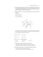
30.1 Is the current intercepted by the surface equal to the
current encircled by the closed path (a) in Figure 30.2a and
(b) in Figure 30.2b?

Figure 30.1 Current-carrying wire encircled by a closed path. Surfaces A
and B both span the path. Surface A lies completely in the plane of the path.
Surface B extends as a hemisphere whose rim is the path.
surface A

surface B

Figure 30.2 Checkpoint 30.1.
(a)
surface
I

I

1

2

closed path

(b)
closed path


surface

I

Checkpoint 30.1 shows that the current encircled by a
closed path is equal to the current that is intercepted by any
surface that spans the path, provided we keep track of the
directions in which each interception takes place. Ampère’s
law can equally well be applied to the current encircled by
a closed path and to the current intercepted by any surface
spanning that closed path.
Now consider inserting a capacitor into our currentcarrying wire while continuing to supply a constant current I to the wire. (That is, the capacitor is being charged.)
Figure 30.3a again shows two surfaces A and B spanning
the same closed path. The line integral of the magnetic
field around the closed path does not depend on the choice
of surface spanning the path. However, while the capacitor is charging, surface A is intercepted by a current I but
Figure 30.3 Capacitor being charged by a current-carrying wire. (a) The
closed path of interest encircles the wire. Surface A intercepts the current,
but surface B passes between the capacitor plates and does not intercept the
current. (b) The closed path of interest lies between the capacitor plates.
Surface A also lies between the plates and does not intercept the current,
but surface B intercepts the current.
(a)
surface A
(intercepts
current)
I

(b)

surface B (does not
intercept current)
I

surface A (does not
intercept current)
I

I

closed path

3

closed path 1

capacitor plates

closed path 2

surface B
(intercepts
current)
I


www.downloadslide.com
30.1 MagnetiC Fields aCCoMpany Changing eleCtriC Fields

surface B, which passes between the capacitor plates, is not

intercepted by any current. If we choose a closed path that
lies between the capacitor plates (Figure 30.3b), a similar
difficulty arises. Surface A intercepts no current, while surface B intercepts the current I.
In the case of a capacitor, therefore, the equivalence
between encircled current and current intercepted by a
surface spanning the encircling path doesn’t hold. Surface B
in Figure 30.3a would lead us to conclude that the line
integral of the magnetic field around closed path 1 is zero.
Because symmetry requires the magnetic field to always
be tangent to the path and have the same magnitude all
around the path, the line integral being zero means there
is no magnetic field at the location of closed path 1 (even
though the path encircles a current). Conversely, surface B
in Figure 30.2b suggests there is a magnetic field at the
location of closed path 2, even though that path encircles
no current. Experiments do indeed confirm that there is a
magnetic field in and around the gap between the plates of
the charging capacitor. So only the surfaces that intersect
the wires leading to the capacitor appear to provide the
correct value of Ienc in Ampère’s law for both closed paths
in Figure 30.3.
Why must there be a magnetic field in and around the
gap between the plates of the charging capacitor? Although
there is no flow of charged particles between the plates of
the capacitor, there is an electric field (Figure 30.4). Let
us examine this electric field in more detail in the next
checkpoint.
30.2 (a) While the capacitor of Figure 30.4 is being
charged, is the current through the wire leading to or from
the capacitor zero or nonzero? Is the electric field between the

plates zero or nonzero? Is it constant or changing? (b) Answer
the same questions for the capacitor fully charged.

Figure 30.4 Capacitor being charged by a current-carrying wire. The
electric field between the plates is shown. Closed path 1 encircles the current through the wire; closed path 2 encircles the electric field between the
capacitor plates.
closed path 1

I

closed path 2
E

I

Figure 30.5 Parallels between (a) the electric field that accompanies a
changing magnetic field and (b) the magnetic field that accompanies a
changing electric field.
(a)

(b)

Changing
E-field c

ccauses a
B-field.

Changing
B-field c


ccauses an
E-field.

S

∆E

S

∆B
S

Direction of B is given by right-hand
current rule, where “current”S is taken
to be in same direction as ∆E.

S

Direction of E is given
by Lenz’s law.

change, and the changing electric field between the capacitor plates acts in a way similar to the current that causes
this change:
A changing electric field is accompanied by a magnetic field.

When the capacitor is fully charged, the current I into
and out of the capacitor is zero, and there is no magnetic
field surrounding the wires to the capacitor. Between the
capacitor plates, the electric field is no longer changing, and

the magnetic field is zero.
There are strong parallels between the electric field that
accompanies a changing magnetic field and the magnetic
field that accompanies a changing electric field, as Figure 30.5
illustrates. Experiments show that the electric field lines that
accompany a changing magnetic field form loops encircling
the magnetic field, just as the magnetic field lines that
accompany a changing electric field form loops encircling
the electric field.
As we discussed in Section 27.3, the magnetic field
surrounding a current-carrying wire forms loops that are
clockwise when viewed looking along the direction of the
current. The direction of these loops can be described by
the right-hand current rule: Point the thumb of your right
hand in the direction of the current, and your fingers curl

ConCepts

The answers to Checkpoint 30.2 suggest that the magnetic field between the plates of the charging capacitor
arises from the changing electric field. The current to the
capacitor causes the electric field between the plates to

801


www.downloadslide.com
802

Chapter 30  Changing eleCtriC Fields


in the direction of the magnetic field. Similarly, the direction of the loops formed by the magnetic field lines that
accompany a changing electric field are given by the righthand
current rule, taking the change in the electric field,
S
∆E, as the “current.” If we take this changeS in the electric
field into account in Figure 30.3, treating ∆E like a current,
the inconsistency we encountered before vanishes:
Either a
S
current or a change in the electric field, ∆E, is intercepted
by the surface, and so for all surfaces spanning the paths we
conclude that there is a magnetic field.
30.3 Consider disconnecting a charged capacitor from
its source of current and allowing it to discharge (to release its
charge into an external circuit). During discharge, the current
reverses direction (relative to its direction when the capacitor
was charging), but the electric field between the plates does not
change direction. How does the direction of the magnetic field
between the plates compare to the direction when the capacitor
was charging? Does the right-hand current rule apply?
example 30.1 Capacitor with dielectric
Consider a capacitor being charged with a constant current I
and a dielectric between the plates. Is the magnitude of the
magnetic field around a closed path spanning the capacitor
(such as closed path 2 in Figure 30.4) any different from what it
would be without the dielectric? Why or why not?
❶ GEttinG startEd I begin by making a two-dimensional
sketch of the capacitor, indicating the position of the closed
path (Figure 30.6).


ConCepts

Figure 30.6

❷ dEvisE plan To determine the magnetic field magnitude
at any position along the closed path, I need to examine the
current and the changing electric field intercepted by a surface
spanning the closed path.
❸ ExEcutE plan If I consider a flat surface through the closed
path (surface A in Figure 30.6), the surface intersects the dielectric. While the capacitor is charging, the dielectric is being polarized: Negative charge carriers in the dielectric are displaced
in one direction, and positive charge carriers are displaced in
the opposite direction. This displacement of charge carriers

corresponds to a current. Surface A also intercepts a changing
electric field. However, without further information about the
capacitor, I can determine neither the current nor the electric
field between the capacitor plates, which is affected by the presence of the dielectric. Surface A therefore doesn’t permit me
to compare the magnetic field magnitude to what it would be
without the dielectric. I therefore draw another surface, making
this surface loop around one of the capacitor plates (surface B
in Figure 30.6). This surface intercepts only the wire leading
from the capacitor, and I know that the current through the
wire is unchanged by the presence of the dielectric. The fact
that the current through this wire is unchanged tells me that the
effective current in the region containing the dielectric is also
unchanged. Therefore, the magnetic field must be the same as it
would be without the dielectric. ✔
❹ EvaluatE rEsult Intuitively I expect the magnetic field
magnitude around my closed path to be unchanged when the
magnetic field magnitude around the wires attached to the

capacitor is unchanged. The electric field between the capacitor plates gives rise to a displacement of charge carriers within
the dielectric and thus affects the electric field between the
capacitor plates, but apparently everything adds up to yield, for
a given current through the capacitor, the same magnetic field
magnitude outside the capacitor for a given current to the
capacitor regardless of the presence or absence of the dielectric.

We now have a complete picture of what gives rise to
electric and magnetic fields and on what kind of charged
particle these fields exert forces. table 30.1 summarizes
the properties of electric and magnetic fields. Note the
remarkable symmetry between the two. Each type of field
is produced by charged particles and accompanies a changing field of the other type. Electric fields are produced by
charged particles either at rest or in motion, but magnetic
fields are produced only by charged particles in motion.
Likewise, any charged particle—at rest or in motion—is
subject to a force in the presence of an electric field, but
only charged particles in motion are subject to forces in a
magnetic field.
table 30.2 summarizes what we know about the field
lines for electric and magnetic fields. The most striking difference between electric and magnetic fields is that magnetic field lines always form loops but electric field lines do
table 30.1 Properties of electric and magnetic fields

 

Electric
field

Magnetic
field


associated with

charged
particle

moving charged
particle

 

changing
magnetic field

changing
electric field

exerts force on

any charged
particle

moving charged
particle


www.downloadslide.com
30.2 Fields oF Moving Charged partiCles
table 30.2 Electric and magnetic field lines


 

lines emanate from
or terminate on
loops encircle
 

Electric
field

Magnetic
field

charged
particle

–

–

moving charged
particle

changing
magnetic field

changing
electric field

not always form loops. This is a direct consequence of the

difference in the sources of these fields. Magnetic field lines
must form loops because there is no magnetic equivalent of
electrical charge—no magnetic monopole (see Section 27.1).
Instead, magnetic fields arise from current loops that act as
magnetic dipoles.
Electric and magnetic field lines that accompany changing fields both form loops around the changing field. When
particles serve as the field sources, however, the difference
between magnetic and electric fields is evident: Electric field
lines emanate or terminate from charged particles, while
magnetic field lines always form loops around moving
charged particles (currents).
We shall return to these ideas quantitatively in Section 30.5.
30.4 The neutron is a neutral particle that has a magnetic
dipole moment. What does this nonzero magnetic dipole moment tell you about the structure of the neutron?

30.2 Fields of moving charged particles

Before examining the electric fields of accelerating
charged particles, let’s consider the electric fields generated
by charged particles moving at constant velocity. Figure 30.7
shows the electric field of a stationary charged particle and
of the same particle moving at constant high speed. (By
high speed, I mean a speed near enough the speed of light
for relativistic effects to become important.)
The electric field of the stationary particle is spherically
symmetrical; the electric field of the moving particle is still
radial but definitely not spherically symmetrical. In this
electric field, the field lines are sparse near the line along
which the particle travels and are clustered together in the
plane perpendicular to the motion. (This clustering is a

relativistic effect and takes place for the same reason that
objects moving at relativistic speeds appear shorter along the
direction of motion, as discussed in Sections 14.3 and 14.6.)
Consequently, the electric field created by the moving particle is strongest in that perpendicular plane. The faster the
particle moves, the more the electric field lines bunch up in
the transverse direction.
Keep in mind that as the particle moves at constant
speed, the electric field lines move with it. At any instant,
the electric field lines point directly away from the position
of the particle at that instant. This means that as the particle
moves, the electric field at a given position changes.
Because the particle in Figure 30.7b is moving, it is like a
tiny current; it has a magnetic field that forms loops around
its direction of travel, as shown in Figure 28.2b. The particle
in Figure 30.7a does not have a magnetic field because it is
at rest.
Now let’s consider a particle that is initially at rest and
then
(a) is suddenly set in motion. The electric field of this
particle is shown at three successive instants in Figure 30.8
on the next page. Figure 30.8b and c show something we
have not seen before: electric
field lines that do not point
S
S
v = 0 particle that is their source
directly away from the charged
but instead are disrupted by sharp kinks. What is more,
these kinks, which appear when the particle accelerates
(just after Figure 30.8a), do not go away once the particle


Figure 30.7 Electric field line pattern of a charged particle (a) at rest and (b) moving to the right with
speed v (v is a significant fraction of the speed of light). For the moving particle, the electric field lines
cluster around the plane perpendicular to the direction of motion.
(a)

(b)

S

S

v=0
S

v

(b)

ConCepts

We have seen that capacitors generate changing electric fields
when charging or discharging. What else produces changing
electric fields? One answer to this question is: changes in
the motion of charged particles.

803


S


804

S

S

v=0

www.downloadslide.com
S

v=0

Chapter 30  Changing eleCtriC Fields

Figure 30.8 Electric field line pattern of a particle (a) initially at rest, (b) accelerating to speed v, and
(c) moving at constant speed v. In (b) and (c), the ring of kinks in the electric field lines traveling outward
from the particle corresponds to an electromagnetic wave pulse. Note that the speed v is smaller than the
speed of the particle in Figure 30.7, indicated by the shorter arrow. Consequently, the electric field lines
here are less sharply bunched around the vertical.
electric field line pattern of charged particle at rest:

shortly after particle accelerates to constant speed:

shortly after particle
(b)accelerates to constant speed:

(a)
(b)

S

S

v=0

S

v
S

v

shortly after particle accelerates to constant speed:

as particle continues at constant speed:

as particle continues
(c)at constant speed:

(b)
(c)

S

v

inner region:
pattern caused by
particle moving

at constant speed

ConCepts

(c)

inner region:
pattern caused by
particle moving
at constant speed

as particle continues at constant speed: ring of kinks: caused
by particle’s acceleration;
electromagnetic pulse

reaches its final constant speed. Instead, they travel radiinner
region:
ally
out
from the location where the particle was
when it
S
v
pattern moving.
caused by
started
particle moving
Where do these kinks in the electric field pattern come
at constant speed
from? They arise because the electric field cannot change

instantaneously everywhere in space to reflect changes in
the source particle’s motion. Remember that field lines
extend infinitely far away from the particles that are their
outer region: pattern
ring of kinks: caused
sources. If the electric
field associated with
a particle could
still unchanged
by particle’s acceleration;
change immediately
everywhere
in
the
universe
when that
electromagnetic pulse
particle changes its motion, then information about the
change in motion would also be transmitted instantaneously throughout the entire universe. As we saw in
Chapter 14, however, experiments show that such an instantaneous transmission of information does not happen.
Changes in the electric field, and the information that these
changes carry, travel at a finite (though very great) constant
speed. In fact, in vacuum such changes always travel at the

S

v
S

v


ring of kinks: caused
by particle’s acceleration;
outer region: pulse
pattern
electromagnetic
still unchanged

outer region: pattern
still unchanged

same speed regardless of the details of the motion of the
particles that produce them.
At distances that are too great for changes to reach in the
time interval represented in Figure 30.8, the electric field
line patterns in Figure 30.8b and c are still the same as the
pattern of the stationary particle of Figure 30.8a. At distances that can be reached in that time interval, the electric
field line patterns in parts b and c are those of the moving
particle. Kinks form in order to connect these two patterns.
These kinks also form when a particle initially moving
at constant velocity abruptly comes to a stop (Figure 30.9).
The particle, initially moving at velocity v, stops just after
the instant shown in Figure 30.9e. Part f shows the electric
field line pattern of the stationary particle after some time
interval has elapsed.
The electric field line density and consequently the magnitude of the electric field are much greater in the kinks
than elsewhere. The energy density in the kinks region is


www.downloadslide.com

30.2 Fields oF Moving Charged partiCles

805

Figure 30.9 Electric field lines of a charged particle moving at some relativistic speed v. The upper
diagrams show successive instants as the particle moves at constant velocity. The lower diagrams
show the same instants, but the particle slows down to a stop between (e) and ( f ).
(a)

(b)

(c)
Particle moves at constant speed.

S

S

v

(d)

S

v

(e)

v


(f)

Particle moves at constant speed c

cthen slows to a stop between (e) and ( f ).

S

S

v

S

v

S

v=0

Acceleration causes ring of kinks.

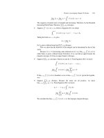
30.5 Estimate the final speed v of the charged particle in Figure 30.8 in terms of the speed of propagation c of
the electromagnetic wave pulse produced by the particle’s
acceleration.

Let us now look at what effect an electromagnetic wave
pulse has on a charged particle. Figure 30.10 on the next page
shows the force exerted on a stationary charged test particle
by the electric field of an accelerated charged particle. At


the first instant shown (Figure 30.10a), before the particle
at the center of the panel is accelerated, the force exerted
by the electric field on the test particle runs along the field
line joining the two particles and points away from the center particle. At the second instant shown (Figure 30.10b),
the center particle has been accelerated, and the wave pulse
created by the acceleration has just reached the test particle.
The force exerted on the test particle is no longer directed
along the line joining the two particles but is directed along
the kinks in the electric field lines. The force therefore has
a component tangential to a circle centered on the original position of the accelerated particle at the center of the
panel. (The exact direction of the force depends on the
magnitude and duration of the acceleration of the accelerated particle.) Moreover, because the electric field line density is large in the region of the kinks, the force is large in
magnitude.
At the final instant shown (Figure 30.10c), the wave
pulse has traveled beyond the test particle and the force
once again points away from the particle. The electric
field line density is much smaller again, and so the magnitude of the force exerted on the test particle is again much
smaller.

ConCepts

therefore greater than the energy density in other parts of
the electric field. As the kinks move, they carry energy away
from the particle. These kinks (and the energy carried by
them) are one of the two parts of electromagnetic waves.
As you might guess, kinks in magnetic field lines are the
other part. Because changing electric fields are accompanied by changing magnetic fields (and vice versa), the two
are always found together. An electromagnetic wave is
thus a combined disturbance in an electric and a magnetic

field that is propagating through space. Because a single
isolated propagating disturbance is called a wave pulse (see
Section 16.1), the kinks that appear in Figures 30.8 are 30.9
are electromagnetic wave pulses.


www.downloadslide.com
806

Chapter 30  Changing eleCtriC Fields

Figure 30.10 Force exerted on a stationary charged test particle by the
electric field of an accelerated charged particle.
stationary charged test particle
(a)

S

F tE

S

S

v=0

(b)

S


F tE

S

v

(b) Yes. Once the pulse arrives at the rod, the electric field in
the rod points downward, accelerating positively charged particles downward and causing a downward current. ✔
❹ EvaluatE rEsult Because the particle being accelerated is
negatively charged, it makes sense that it pulls positive charge
carriers in the rod along (with a delay caused by the time interval it takes the wave pulse to travel to the rod). In practice,
electrons in the rod are accelerated upward, but the result is the
same as what I describe for positive charge carriers.

(c)

S

F tE

the electric field of the negatively charged particle create a current through the rod (a) at the instant shown in the figure, before the electromagnetic wave pulse created by the acceleration
reaches the rod, and (b) at the instant the pulse reaches the rod?
If you answer yes in either case, in which direction is the current through the rod?
❶ GEttinG startEd A current is created when charge carriers
in the rod flow through the rod. For the carriers to flow, a force
needs to be exerted on them.
❷ dEvisE plan To determine whether there is a current
through the rod, I must determine if the electric field is oriented
in such a way as to cause a flow of charge carriers through the
rod. Even though in a metallic rod only electrons are free to

move, I can pretend that only positive charge carriers are free
to move because as I saw in Section 27.3, my answer is independent of the sign of the mobile charge carriers.
❸ ExEcutE plan (a) No. Before the pulse reaches the rod,
the electric field is constant and so the rod is in electrostatic
equilibrium. Therefore the electric field magnitude inside the
rod is zero, so no charge carriers in the rod flow at the instant
shown. ✔

S

v

30.6 In Figure 30.10, in which regions of space surrounding the accelerating particle does a magnetic field occur?

ConCepts

30.3 oscillating dipoles and antennas

example 30.2 electromagnetic wave pulse
A particle carrying a negative charge is suddenly accelerated in
a direction parallel to the long axis of a conducting rod, producing the electric field pattern shown in Figure 30.11. Does
Figure 30.11 Electric field of an accelerated particle near a conducting rod, before the wave pulse reaches the rod. (The electric field lines
bend in near the conducting rod due to the rearrangement of charge
carriers at the surface of the rod.)

S

v

The wave pulse we have just considered is a brief, one-time,

propagating disturbance in the electric field, analogous to
the disturbance created when the end of a taut rope is suddenly displaced (as in Figure 16.2, for instance). Just as a
harmonic wave can be generated on a rope by shaking the
end of the rope back and forth in a sinusoidal fashion, a
harmonic electromagnetic wave can be generated when a
charged particle oscillates sinusoidally. Figure 30.12 shows
the electric field of a charged particle undergoing sinusoidal oscillation. This electric field consists of periodic kinks
traveling away from the particle in a wavelike fashion.
In practice, isolated charged particles are not common.
More often, positive and negative charged particles are
present together, whether in individual atoms or in solid or
liquid materials. Thus, displacing a positive particle leaves a
negative particle behind, forming an electric dipole. Let us
therefore consider the electric field pattern of an oscillating
dipole.


www.downloadslide.com
30.3 osCillating dipoles and antennas
Figure 30.12 Electric field of a sinusoidally oscillating charged particle.

S

v

The electric field pattern of a stationary electric dipole
with the positive charged particle above the negative
charged particle is shown in Figure 30.13a. What about
the electric field pattern of a stationary dipole made up
of the same charged particles but with their positions

S
switched, so that the dipole moment p—which points
from the negatively charged end to the positively charged
end (see Section 23.4)—has reversed? The corresponding
pattern of electric field lines has the same shape as shown
in Figure 30.13a, but the directions of all the electric field
lines are reversed.
Now let’s work out the electric field pattern of an oscillating dipole, in which the two particles oscillate back and
forth with a period T. We begin by considering the electric

807

field of a dipole that undergoes only a single reversal of its
dipole moment (that is, one-half of a single oscillation)
rather than oscillating continuously. The dipole starts out
as shown in Figure 30.13a at instant t = 0. The charged
particles that constitute the dipole then switch places in a
time interval T>2 (half a cycle) and remain there.
Figure 30.13b shows the electric field pattern at instant
t = T, after the dipole has been at rest in its new orientation
for a time interval T>2. We can divide the space surrounding the dipole into the three regions shown. First consider
the region sufficiently close to the dipole that the electric
field is just the electric field of the stationary dipole in its
new orientation. If we denote the speed at which changes in
the electric field travel outward by c and the dipole has been
stationary for a time interval T>2, this innermost region
occupies a circle of radius R = cT>2. (The origin of our
coordinate system is the center of the dipole, midway between the two particles.) Inside this circle, the electric field
is that of the stationary dipole, the same shape as shown in
Figure 30.13a but with the electric field line directions

reversed.
Now consider the region sufficiently far away that no information about the motion of the dipole has reached it yet.
This region lies outside a circle of radius R = cT. In this
region, the electric field pattern is identical to that shown in
Figure 30.13a, the electric field of the original dipole before
it flipped over.
In the highlighted region of Figure 30.13b between these
two circles, the electric field pattern is not dipolar. Because
there are no charged particles in this region, the electric
field lines cannot begin or end here. Instead, they must be
connected to the electric field lines in the inner and outer
regions. Consequently the electric field lines split into two
disconnected sets: a set that emanates from the ends of the
dipole and a set of loops detached from the dipole.

Figure 30.13 (a) Electric field of a stationary electric dipole in which the positive particle lies above
the negative particle. (b) Electric field of the same dipole after the dipole moment has reversed and
the charged particles have returned to rest.
(b) Field shortly after dipole has reversed
R = cT
t=0

t=T
R = cT> 2

S

p

S


p

R 6 cT>2: electric field
of dipole in reversed
orientation
electric field of reversing
dipole; field lines connect
inner and outer regions
R 7 cT: electric field of dipole in original orientation

ConCepts

(a) Electric field of stationary electric dipole


www.downloadslide.com
808

Chapter 30  Changing eleCtriC Fields

Figure 30.14 Snapshots of the electric field pattern of a sinusoidally
oscillating dipole at time intervals of T>8 (where T is the period of
oscillation).
S

p

t=0
S


p

t = 18 T

S

S

t=

1
4T

p=0

30.7 (a) If Figure 30.14 shows the oscillating electric
field pattern at its actual size, estimate the wavelength of the
electromagnetic wave. (b) If the wave is traveling at speed
c = 3 × 108 m>s, what is the wave frequency? (c) How long
does one period last?

t = 38 T

So far we have focused on the electric field pattern of
this electromagnetic wave because it is natural to think
about the electric field of a dipole. However, the changing
electric field of the oscillating dipole is accompanied by a
magnetic field. Consequently, the oscillation produces not
only an electric field but also a magnetic field.


S

p

example 30.3 Magnetic field pattern

t = 12 T
S

p

t = 58 T
S

p

ConCepts

This electric field line pattern can be generalized to the
case of a sinusoidally oscillating dipole (one that doesn’t
stop after half a cycle). Figure 30.14 shows snapshots of the
electric field pattern of such a dipole at time intervals of
T>8. Just as with the single half-oscillation, we see a dipolar
electric field near the dipole. Farther away, the electric field
lines form loops.
Notice how these loops form every half-cycle (that is,
at t = T>4 and t = 3T>4): As the charged particles of the
dipole reach the origin during each oscillation, the electric
field lines pinch off and the loops travel outward like puffs

of smoke. This regular emission of looped electric field
lines is a harmonic electromagnetic wave that travels away
from the dipole horizontally left and right.

t = 34 T

S

S

p=0

Consider the electric field pattern of a sinusoidally oscillating
dipole in Figure 30.14. (a) At t = 34 T, where along the horizontal axis bisecting the straight line connecting the two poles is
the electric field increasing with time? Where is it decreasing?
(b) Based on your answer to part a, what pattern of magnetic
field lines do you expect in the horizontal plane that bisects the
straight line connecting the two poles?
❶ GEttinG startEd Because the dipole oscillates sinusoidally, I expect the electric field to be a sinusoidally oscillating
outward-traveling wave. The wave is three-dimensional, but
the problem asks only about the electric field along the dipole’s
horizontal axis, so a one-dimensional treatment of this wave
suffices. Because the wave is three-dimensional, the amplitude
decreases as 1>r as the wave travels outward (see Section 17.1),
but I’ll ignore the decrease over the small distance over which
the wave propagates in the figure.
❷ dEvisE plan I know from Chapter 16 that a one-dimensional
sinusoidal wave can be represented by a sine function both in
space and in time. (The wave function shows the value of the
oscillating quantity as a function of position at a given instant

in time, and the displacement curve shows the oscillating
quantity as a function of time at a given position.) I can use the
information shown in Figure 30.14 to draw the wave function
for the electric field at t = 34 T. Once I have the wave function
and know which way the wave is traveling, I can determine
where the electric field increases. Because a changing electric
field causes a magnetic field, I can use the information from
part a to solve part b.


www.downloadslide.com
30.3 osCillating dipoles and antennas

❸ ExEcutE plan (a) Because the problem asks for information
at the instant t = 34 T, I begin by copying the right half of the
bottom electric field pattern of Figure 30.14 (Figure 30.15a).
(The left half is simply the mirror image of the right half.) I
draw a rightward-pointing horizontal axis through the center
of the dipole and denote this as the z axis. I see that the electric
field points downward parallel to the vertical axis (which I take
to be the x axis) in the region between the dipole and the center
of the first set of electric field loops. In the region between the
centers of the first and the second set of loops, the electric field
points upward. Because the electric field must vary sinusoidally,
I can now sketch how its x component varies with position
along the horizontal axis (Figure 30.15b).
Figure 30.15

809


the derivative of Ex with respect to z is positive (shaded regions)
and up when it is negative (unshaded regions). ✔
(b) The direction of the magnetic field is determined by the
right-hand current rule,
taking the direction of the change in
S
the electric field ∆E as the “current.” Pointing
the thumb of
S
my right hand
down
in
the
region
where
∆E
points
down and
S
up where ∆E points up (Figure 30.15d), I see from the way
my fingers curl that the magnetic field lines form loops in the
horizontal (yz) plane that are centered on the vertical black
dashed lines, just like the electric field lines do. Consequently
the magnetic field points out of the page when Ex is positive
and into the page when Ex is negative. If I let the y axis point
out of the page, the y component of the magnetic field must be
positive when Ex is positive and negative when Ex is negative.
I therefore draw a sinusoidally varying function for By as a
function of position (Figure 30.15e). ✔
❹ EvaluatE rEsult My answer shows that the electric and

magnetic fields have the same dependence on time but are
oriented perpendicular to each other. Because the magnetic
field changes, Faraday’s law tells me that it is accompanied
by an electric field. To analyze this electric field I can use an
approach similar to the one I used to determine the magnetic
field. Figure 30.16a shows the magnetic wave traveling outward. The difference between the dashed
and solid curves
S
is the change in the magnetic field ∆B. According to what
I learned in Section 29.6, the direction of the electric field accompanying my changing magnetic field is given by Lenz’s law
and the right-hand dipole rule (Figure 30.16b). Consequently
the electric field points into the page when By is positive and
out of the page when By is negative. Because the x axis points
into the page in this rendering (compare Figures 30.15d and
30.16b), the x component of the electric field must be positive
when By is positive and negative when By is negative, as shown
in Figure 30.16c. The electric field shown in Figure 30.16c is
exactly the electric field I started out with in Figure 30.15b. In
other words, the electric field yields the magnetic field and the
magnetic field yields the electric field, and the two are entirely
consistent with one another.

S

ConCepts

S

B into page B out of page


S

B into page

As the wave travels outward, the wave function of Figure
30.15b moves to the right (dashed curve in Figure 30.15c). The
difference between theS dashed and solid Scurves is the change
in the electric field ∆E (black arrows); ∆E points down when

right-hand dipole rule

right-hand current rule

Figure 30.16

S

E out of
page

S

E into page

S

E out of page
thumbs: direction
S
opposite ∆B

(Lenz’s law)


www.downloadslide.com
810

Chapter 30  Changing eleCtriC Fields

Figure 30.17 Electric and magnetic field pattern of oscillating dipole.
The pink arrows indicate the direction of propagation of the electromagnetic wave pulse. For simplicity, only the fields in the xz and yz planes
are shown.

Figure 30.18 System of two antennas, one that emits electromagnetic
waves and one that receives them. The emitting antenna is supplied with an
oscillating current created by a source of alternating potential difference.
An oscillating current is induced in the receiving antenna by the arriving
electromagnetic wave.

x

emitting
antenna

E

receiving
antenna

I


I

I

I

z
B

y

Oscillating current
causes antenna to
emit oscillating field.

The solution to Example 30.3 suggests that the magnetic
field line pattern is similar to the electric field line pattern,
but perpendicular to it. Figure 30.17 shows the combined
electric and magnetic field pattern of an oscillating dipole.
Traveling electromagnetic waves, like the one shown in
Figure 30.17 are transverse waves (see Section 16.1) because
both the magnetic field and the electric field are perpendicular to the direction of propagation. Also, the electric and
magnetic fields propagate at the same frequency, and both
reach their maxima (or minima) simultaneously; the electric
and magnetic fields are therefore in phase with each other.

ConCepts

30.8 (a) At the origin of the graphs in Figure 30.15, the
electric field is zero, but there is a current due to the motion of

the charged particles that constitute the dipole. Is this current
upward, downward, or zero at the instant shown in Figure 30.15?
(b) Is this current (or the absence thereof) consistent with the
magnetic field pattern shown in Figure 30.17?

In the wave shown in Figure 30.17, not only are the electric and magnetic fields perpendicular to each other, but
throughout the entire wave the electric field has no component perpendicular to the xz plane. (The magnetic field, in
contrast, is always perpendicular to this plane.) By convention the orientation of the electric field of an electromagnetic wave as seen by an observer looking in the direction
of propagation of the wave is called the polarization of
the wave. An observer looking at the dipole in Figure 30.17
would say that the wave from the dipole is polarized along
the x axis. Because the electric field oscillation from the dipole in Figure 30.17 retains its orientation as it travels in
any given direction, the wave is said to be linearly polarized.
In certain cases the polarization of an electromagnetic wave
rotates as it propagates, and the wave is said to be circularly
or elliptically polarized.
We have seen that oscillating dipoles generate electromagnetic waves by accelerating the oppositely charged
particles that make up the dipole in a periodic manner.
Practically speaking, how can we cause charged particles,
in a dipole or anything else, to accelerate periodically?
One common approach is to apply an alternating potential

Oscillating field causes
oscillating current
through antenna.

difference to an antenna, which is a device that either emits
or receives electromagnetic waves. The alternating potential
difference drives charge carriers back and forth through the
antenna, thereby producing an oscillating current through

the antenna.
Antennas that emit electromagnetic waves are designed
in many ways to produce a variety of electric and magnetic
field patterns. The simplest design is two conducting rods
connected to a source of alternating potential difference
(Figure 30.18). Because of the alternating potential difference, the ends of the antenna are oppositely charged and
cycle between being positively charged, neutral, and negatively charged.
When the top end of the antenna is positively charged
and the bottom end is negatively charged, the electric
field of the antenna points down. When the charge distribution is reversed, the electric field points up. As the
charge distribution oscillates, the electric field adjacent to
the emitting antenna also oscillates. This changing electric
field is accompanied by a changing magnetic field, and the
disturbance in the fields travels away from the emitting
antenna in the same manner as the electromagnetic wave
of Figures 30.14, 30.15, and 30.17.
If the length of each rod in an emitting antenna is exactly
one-quarter of the wavelength of the electromagnetic wave
emitted, the electric fields produced strongly resemble the
dipole fields of Figure 30.17. Such an antenna is often called
a dipole antenna; it is also called a half-wave antenna because
the length of the two rods is equal to half a wavelength.
In antennas that receive electromagnetic waves, the oscillating electric field of the wave causes charge carriers in
the antenna to oscillate, as discussed in Example 30.2. This
produces an oscillating current (shown schematically in
Figure 30.18) that can be measured. When operated in this
mode, the antenna is said to be receiving a signal.
30.9 To maximize the magnitude of the current induced
in a receiving antenna, should the antenna be oriented parallel
or perpendicular to the polarization of the electromagnetic wave?



www.downloadslide.com
selF-quiz

811

self-quiz
1. Suppose the current shown in Figure 30.19
discharges
S
S
S
the capacitor. What are the directions of E, ∆E, and B
between the plates of the discharging capacitor?

Figure 30.19

2. A positively charged particle creates the electric field
shown in Figure 30.20. When the kinks in the electric
field lines reach the rod, what is the direction of the
current induced in the rod?
3. For the oscillating dipole of Figure 30.14, sketch the
electric field pattern at t = 54 T.

Figure 30.20

4. In the electric field pattern for a sinusoidally oscillating dipole shown in Figure 30.21, what are (a)Sthe
direction of the change in the electric field ∆E at
point C as the electric field propagates and (b) the

direction of the magnetic field loop near C?

Figure 30.21

I

C

answers
1. The current brings positive charge carriers to the left plate and removes them from the right plate. For the caS
pacitor to discharge, the left plate must be negatively charged and the right
one positively charged; this means E
S
points left. The electric field decreases as the capacitor discharges, so ∆E is to the right (just as the current is).
The magnetic field lines are circular and centered on the axisSof the capacitor in a direction given by the righthand current rule with the thumb along the direction of ∆E. That is, the magnetic field lines are clockwise
looking along the direction of the current.
2. Because the particle carries a positive charge, the electric field lines radiate outward. The electric field in the
kinks therefore points up, and so the kinks induce an upward current through the rod.
Figure 30.22

4. (a) The loops passing at C travel to the
left. At the instant shown, the electric
field is close to zero, but as the pattern
S
moves to the left, the electric Sfield lines point downward at C, so ∆E is down. (b) The thumb of your right hand
aligned in the direction of ∆E makes your fingers curl in the direction of the magnetic field: clockwise viewed
from the top.

self-quiz


3. See Figure 30.22. Because the loops
move outward and a new pair of loops
forms every half-period, the pattern now
has three loops. Note in Figure 30.14
that the loops closest to the dipole at
t = 14 T and t = 34 T have the same shape
but opposite directions. Half a period
after t = 34 T, at t = 54 T, the loops closest
to the dipole again have the same shape
(and the same direction as at 14 T). Likewise, at t = 54 T the second closest loops
curl in the direction opposite the direction at 34 T.


www.downloadslide.com
812

Chapter 30  Changing eleCtriC Fields

Figure 30.23 Capacitor being charged by a
current-carrying wire. Because surfaces A and
B both span the closed path shown, either surface can be used to calculate the magnetic field
around the path. Ampère’s law must be the same
in either case.
surface A

surface B

I

I

q

closed path

30.4 Displacement current
The work we did with Ampère’s law in Sections 28.4 and 28.5 dealt only with the
magnetic field associated with an electric current. As we saw in Section 30.1,
though, magnetic fields also accompany changing electric fields, a phenomenon
not covered by our Chapter 28 form of Ampère’s law. Let us now see how the
quantitative formulation of Ampère’s law must be modified to account for the
magnetic fields that accompany changing electric fields.
To do this, consider the charging capacitor in Figure 30.23. Ampère’s law
relates the integral of the magnetic field around a closed path to the current
intercepted by a surface spanning the path (Eq. 28.1). Applying Ampère’s law to
surface A in Figure 30.23, we have

#
C B d/ = m0I.
S

S

(30.1)

For surface B, however, the right-hand side of Eq. 30.1 is zero because the current is zero in the gap between the capacitor plates. As we discussed in Section
30.1, there is a change in the electric field between the capacitor plates, so surface B does not intercept a current, but it does intercept a change in electric flux.
Let us therefore generalize Ampère’s law by adding to the right side a term that
depends on this change in electric flux.
We choose this term so that when we apply the generalized version of
Ampère’s law to the capacitor shown in Figure 30.23, for example, the magnetic

field around the designated path is the same whether we calculate it from the
current intercepted by surface A or from the change in electric flux dΦE >dt
through surface B.
To obtain this generalizing term, let’s determine a mathematical relationship
between dΦE >dt through surface B and the current to the plates. First, note that
the change in electric flux is related to the change in the charge q on the plates,
which, in turn, is related to the current I to the plate. Consider the closed surface
surrounding the left capacitor plate in Figure 30.23 made up by surfaces A and
B combined. Applying Gauss’s law to this closed surface, we find that the electric
flux through it is
S
# S q
CAE B dA = P0 ,
+

(30.2)

where q is the charge on the capacitor plate. Because the electric field is confined
to the region between the plates, the electric flux through surface A is zero
(Figure 30.23) and so

Quantitative tools

S
S
S
S
# S
# S
# S

# S q
CAE B dA = 3AE dA + 3BE dA = 3BE dA = P0 .
+

(30.3)

If we denote the electric flux through surface B by ΦE, we see from Eqs. 30.3
that q = P0ΦE. The rate of change of the charge on the capacitor plates, dq>dt, is
equal to the current supplied to the capacitor, so
IK

dq
dΦE
= P0
,
dt
dt

(30.4)

which is the relationship we were looking for.
If we substitute Eq. 30.4 in the right side of Eq. 30.1, we obtain
S
dΦE
# S
C B d/ = m0P0 dt .

(30.5)



www.downloadslide.com
30.4 displaCeMent Current

813

We can now use this expression to determine the line integral of the magnetic
field around the closed path in Figure 30.23 by evaluating the change in electric
flux through
surface
B. Because the right side of Eq. 30.5 is equal to m0I, we obS
S
tain for A B # d/ the same value we found using the original form of Ampère’s
law with the current intercepting surface A.
To account for both a current and a changing electric flux, we generalize
Ampère’s law as follows:
S
dΦE
# S
C B d/ = m0Iint + m0P0 dt .

(30.6)

This equation holds for any surface spanning a closed path and is sometimes
called the Maxwell-Ampère law, in honor of the Scottish physicist James Clerk
Maxwell (1831–1879), who first introduced the additional term in Eq. 30.6. To
reflect the fact that we must only include the current intercepted by the surface,
not the current encircled by the integration path, we write Iint rather than Ienc .
The quantity on the right side of Eq. 30.4 is called the displacement current:
Idisp K P0


dΦE
.
dt

(30.7)

As you can see from Eq. 30.4, the SI units of the displacement current are indeed
those of a current. The name is somewhat misleading because the derivation
holds for a capacitor in vacuum where no charged particles are present in the
space between the plates. Even if the term is somewhat of a misnomer, it is still
useful to associate the change in the electric field with a “current” to determine
the direction of the magnetic field accompanying a changing electric field. As
we argued in Section 30.1, the direction of this
displacement current is the same
S
as that of the change in the electric field ∆E. We can then use the right-hand
current rule to determine the direction of the magnetic field from the displacement current (see, for example, Figure 30.5).
Using Eq. 30.7, we can write Eq. 30.6 in the form

#
C B d/ = m0(Iint + Idisp).
S

S

Figure 30.24 Checkpoint 30.10.
P
decreasing E-field

(30.8)


S

30.10 The parallel-plate capacitor in Figure 30.24 is discharging so that the electric field between the plates decreases. What is the direction of the magnetic field (a) at
point P above the plates and (b) at point S between the plates? Both P and S are on a line
perpendicular to the axis of the capacitor.

example 30.4 a bit of both
Figure 30.25 Example 30.4.
P

I

R

E
I

(Continued)

Quantitative tools

The parallel-plate capacitor in Figure 30.25 has circular plates of
radius R and is charged with a current of constant magnitude I.
The surface is bounded by a circle that passes through point P
and is centered on the wire leading to the left plate and perpendicular to that wire. The surface crosses the left plate in the
middle so that the top half of the plate is on one side of the surface and the bottom half is on the other side. Use this surface
and Eq. 30.6 to determine the magnitude of the magnetic field
at point P, which is a distance r = R from the capacitor’s horizontal axis.



www.downloadslide.com
814

Chapter 30  Changing eleCtriC Fields

❶ GEttinG startEd The surface intercepts both a current
(through the plate) and a changing electric field (between the
plates). To apply Eq. 30.6, I must therefore determine both the
current and the electric flux intercepted by the surface.
There also is a simple way to obtain the answer to this
question: Ampère’s law (Eq. 30.1). If I take the circle through
point P centered on the wire and perpendicular to it as the
integration path, then the integral on the left side of Eq. 30.1 is
equal to the magnitude of the magnetic field times the circumference of the circle: 2pRB. The path encircles the current I,
so Ampère’s law gives me 2pRB = m0I and B = m0I>(2pR).
Because the magnetic field magnitude cannot depend on the
approach used to calculate it, I should obtain the same result
using Eq. 30.6 and the surface in Figure 30.25.
❷ dEvisE plan The left side of Eq. 30.6 is identical to the left
side of Eq. 30.1 and therefore equal to 2pRB. To evaluate the
right side of Eq. 30.6, I must determine both the ordinary current and the displacement current intercepted by the surface.
❸ ExEcutE plan If the surface intercepted the entire electric
flux between the plates, the displacement current term on the
right side of Eq. 30.6 would be equal to m0I. The surface intercepts only half of the electric flux, however, so the displacement
current is
P0

dΦE 1
= 2 I.

dt

Because the top half of the plate is to the right of the surface, the
current going to the top half of the plate must cross the surface.
The current intercepted by the surface is thus 12 I, and the right
side of Eq. 30.6 becomes
m0Iint + m0P0

dΦE
= m0112 I2 + m0112 I2 = m0I.
dt

(1)

Substituting the right side of Eq. 1 into the right side of Eq. 30.6,
I have 2pRB = m0I and so B = m0I>(2pR), which is the same
value I got using Eq. 30.1. ✔
❹ EvaluatE rEsult It’s reassuring to see that the magnetic
field magnitude at P does not depend on the choice of surface
spanning the integration path. I can easily modify the argument
above to show that any other surface that intercepts the left plate
gives the same result. For example, a surface that intercepts onequarter of the plate, as in Figure 30.27, intercepts one-quarter
of the electric flux, and so the displacement current is only I>4.
This surface intercepts the current twice: Where the surface intersects the wire, the current I crosses the surface from left to
right, and where the surface intersects the plate, one-quarter of
the current crosses the surface in the other direction, for a total
contribution of 34 I. Again the sum of the ordinary and displacement currents intercepting the surface is I.
Figure 30.27

Next I need to determine how much current is intercepted by

the surface. To charge the plate uniformly, the current must
carry charge carriers evenly to the two halves of the plate—
half of the charge carriers go to the top half of the plate and
the other half go to the bottom half of the plate (Figure 30.26).
Figure 30.26

Quantitative tools

example 30.5 Magnetic field in a capacitor
A parallel-plate capacitor has circular plates of radius
R = 0.10 m and a plate separation distance d = 0.10 mm.
While a current charges the capacitor, the magnitude of the
potential difference between the plates increases by 10 V>ms.
What is the magnitude of the magnetic field between the plates
at a distance R from the horizontal axis of the capacitor?
❶ GEttinG startEd As the capacitor is charging, there is a
changing electric flux between the plates, so the electric field
between the plates is changing. This changing electric field is
accompanied by a magnetic field.

❷ dEvisE plan Equation 30.6 relates the magnetic field to a
changing electric flux. To work out the left side of Eq. 30.6, I
chose a circular integration path centered on the horizontal axis
of the capacitor so that I can exploit the circular symmetry of
the problem. To work out the right side of Eq. 30.6, I need to
determine the rate of change of the electric flux through an
appropriate surface spanning the integration path. I choose the
simplest possible surface: a flat surface parallel to the plates
(Figure 30.28). To calculate the change in electric flux intercepted by this surface, I need to determine the magnitude of



www.downloadslide.com
30.4 displaCeMent Current

Figure 30.28

Because Vcap = Ed, I can write E = Vcap >d and so
B=

m0P0R dVcap
2d
dt

815

(2)

B = (4p × 10-7 T # m>A)(8.85 × 10-12 C2 >N # m2)
×

0.10 m
10 V
2(0.10 × 10-3 m) 1.0 × 10-6 s

= 5.6 × 10-8 T,
the (uniform) electric field between the plates. In Example 26.2
I determined that the magnitude of the electric field between
the plates is related to the plate separation distance d and
the magnitude of the potential difference between the plates:
Vcap = Ed.

❸ ExEcutE plan Because the electric field between the plates
is uniform and perpendicular to the plates, the electric flux
ΦE through the surface I chose is ΦE = EA = EpR2, where
A = pR2 is also the area of the capacitor plates. The time rate of
change of the electric flux is then given by
dΦE
dE
= pR2 .
dt
dt

where I have used the Eq. 25.16 definition of the volt, 1 V K
1 J>C K 1 N # m>C and the Eq. 27.3 definition of the ampere
1 C K 1 A # s to simplify the units. ✔
❹ EvaluatE rEsult The magnetic field magnitude I obtain
is very small, in spite of the substantial rate at which the potential difference between the plates increases. I have no way of
knowing whether my numerical result is reasonable or not, but
what I can do to evaluate the result is use another method to
obtain an expression for B. Because my flat surface intercepts
all the electric flux, I know that the magnitude of the magnetic field should be the same at all positions a distance R from
the current-carrying wire. I can obtain the current by solving
Eq. 26.1, q>Vcap = C, for the charge q on the capacitor plate and
then using the definition of current, I K dq>dt:

Substituting this result in Eq. 30.6 and setting the current term
equal to zero because no current is intercepted by the surface
I’ve chosen, I get
2 dE
#
.

C B d/ = m0P0pR
S

S

dt

Around my integration path, the magnitude of the magnetic
field is constant, and the left side of this expression simplifies to
2pRB. Solving for B, I obtain
B=

m0P0R dE
.
2 dt

(1)

IK

dq
dt

=C

dVcap
dt

.


Substituting the capacitance of a parallel-plate capacitor
C = P0A>d = P0pR2 >d (see Example 26.2) into this expression,
and then substituting the result into the expression for the magnetic field around a current-carrying wire from Example 28.3,
B = m0I>(2pr) (setting r = R for the distance to the wire), I get
B=

m0P0R dVcap
m0I
=
,
2pR
2d
dt

the same result I obtained in Eq. 2, as I expect.

Note that in Example 30.5 the rate of change of the electric field is very large
(about 1011 V>(m # s)), but the accompanying magnetic field is small. This is not
the case for electric fields that accompany changing magnetic fields, as substantial emfs can be induced by the motion of ordinary magnets.

Quantitative tools

30.11 Consider again the parallel-plate capacitor of Figure 30.23. For circular
plates of radius R, calculate the magnitude of the magnetic field a distance r 6 R from
the horizontal axis of the capacitor (a) between the plates and (b) a short distance to the
right of the right plate.


www.downloadslide.com
816


Chapter 30  Changing eleCtriC Fields

example 30.6 Displacement current in the presence of a dielectric
Suppose a slab of dielectric with dielectric constant k is
inserted between the plates of the capacitor in Figure 30.23
and the capacitor is charged with a current I, as considered in
Example 30.1. How does Eq. 30.6 have to be modified to
account for the dielectric?
❶ GEttinG startEd For a given amount of charge on the
capacitor plates, the presence of a dielectric decreases the magnitude of the electric field between them. As I concluded in
Example 30.1, however, the magnetic field surrounding the
wires that lead to the capacitor wires is determined only by the
current I through the wires and therefore cannot be affected by
the insertion of the dielectric.
❷ dEvisE plan Given that the magnetic field surrounding
the wires cannot be affected by the presence of the dielectric,
the displacement current intercepted by a surface spanning a
circular path around the wire and passing between the capacitor plates (Figure 30.29) should be equal to I, regardless of the
Figure 30.29

presence of the dielectric. By setting the displacement current
through the surface in Figure 30.29 equal to I, I can determine
how the right side of Eq. 30.6 needs to be modified to account
for the presence of the dielectric.
❸ ExEcutE plan As the capacitor charges, the presence of the
dielectric reduces the magnitude of the electric field by a factor
1>k (see Eq. 26.15): E = Efree >k. As a result, the rate of change
of the electric field dE>dt and the rate of change in the electric flux intercepted by the surface dΦE >dt are also reduced by a
factor 1>k. To compensate for this reduction, I need to multiply

dΦE >dt by k in order to make the right side of Eq. 30.4 equal to
I again. Therefore Eq. 30.6 becomes
dΦE
S
# S
C B d/ = m0I + m0P0k dt . ✔

❹ EvaluatE rEsult My modification to Eq. 30.6 is identical
to the modification we made to make Gauss’s law work in dielectrics (Eq. 26.25): In both cases the term containing the electric field or electric flux includes the factor k.

30.5 Maxwell’s equations
With
Maxwell’s
addition of the displacement current P0dΦE >dt to Ampère’s law,
S
S
#
B
d/
=
m
I,
0 we now have a complete mathematical description of electric
A
and magnetic phenomena and the relationship between the two. Let us summarize this description in the absence of a dielectric.
Electric and magnetic fields are defined by Eq. 27.20, which gives the force
exerted on a charged particle moving in an electric field and a magnetic field:
S

S


S

S

Quantitative tools

F = q(E + v × B).

(30.9)

Charged particles are the source of electrostatic fields, and electrostatic field
lines always begin or end on charged particles. We can calculate electric fields
from each individual charged particle if we wish, but when dealing with a distribution of charge that exhibits a certain symmetry (Section 24.4), it is most
convenient to use Gauss’s law (Eq. 24.8) to work out the electric field. Gauss’s law
tells us that the electric flux ΦE through a closed surface (a Gaussian surface) is
proportional to the charge enclosed by the surface:
qenc
S
S
ΦE K C E # dA =
.
P0

(30.10)

Figure 30.30a shows the electric field created by a charged particle, along with a
Gaussian surface enclosing that particle.



www.downloadslide.com
30.5 Maxwell’s equations

817

Figure 30.30 Graphical representation of the physics behind Maxwell’s equations, together with their
mathematical expressions. (a) Electric field surrounding a charged particle and a Gaussian surface
enclosing that particle. Gaussian surfaces can be used to relate the electric field to the enclosed charge.
(b) Magnetic field surrounding a current-carrying wire and a closed surface intercepted by the wire; the
integral of the magnetic field over a closed surface is always zero. (c) Electrostatic field and two closed
paths through that field; the path integral of the electric field around either path must be zero. (d) Steady
magnetic field surrounding a current and two closed paths through that field; the path integral of the
magnetic field is proportional to the encircled current. (e) Changing magnetic field and two closed
paths through it; an electric field accompanies the changing magnetic field; the path integral of this
electric field around either path is nonzero. (f) Changing electric field and two closed paths through it;
a magnetic field accompanies the changing electric field; the path integral of this magnetic field around
either path is nonzero.
(a) Surface integral of electric field (Gauss’s law)

(b) Surface integral of magnetic field (Gauss’s law for magnetism)

S
# S qenc
C E dA = P0

E

#
C B dA = 0
S


B

I

q

closed surface

closed surface

(c) Line integral of constant electric field

(d) Line integral of constant magnetic field (Ampère’s law)

#
C E d/ = 0

E

S

S

#
C B d / = m0Ienc

B

S


q

I

closed path 2

(e) Line integral of changing electric field (Faraday’s law)

closed path 2

(f) Line integral of changing magnetic field (Maxwell’s displacement current)

S
dΦB
# S
C E d / = − dt

S
dΦE
# S
C B d / = P0m0 dt

E

B
closed path 1

closed path 1


closed path 2

closed path 2

S

E out of page, increasing

Quantitative tools

B out of page, increasing

S

closed path 1

closed path 1

S

S


www.downloadslide.com
818

Chapter 30  Changing eleCtriC Fields

Magnetic fields are generated by moving charged particles, commonly in the
form of currents. Unlike electric field lines, magnetic field lines always form loops.

There are no isolated magnetic poles, only magnetic dipoles. Consequently, as
we showed in Chapter 27, the magnetic flux through any closed surface is always
zero (Eq. 27.11):
ΦB K C B # dA = 0.
S

S

(30.11)

Figure 30.30b shows the magnetic field surrounding a current-carrying wire,
along with a closed surface intercepted by the wire.
For electrostatic fields, we showed in Chapter 25 that the path integral of the
electric field around a closed path is zero, which means that when a charged
object is moved around a closed path in an electrostatic field, the work done on
it is zero (Eq. 25.32). This situation is represented in Figure 30.30c. However,
the electric field accompanying a changing magnetic field does work on charged
particles even when those particles travel around closed paths:
S
dΦB
# S
C E d/ = - dt .

(30.12)

Figure 30.30e shows the electric field lines associated with a changing magnetic
field. For such an electric field, no potential can be defined because the path integral of the electric field depends on the path chosen.
Finally, Ampère’s law gives the line integral of the magnetic field produced
by a current (Figure 30.30d). The magnetic field that accompanies a changing
electric field forms loops around the direction of the change in electric field, as

shown in Figure 30.30f. Combining these two contributions to the line integral
of the magnetic field gives us Maxwell’s generalization of Ampère’s law, which is
our Eq. 30.6, repeated here:

Quantitative tools

S
dΦE
# S
C B d/ = m0Iint + m0P0 dt .

(30.13)

Equations 30.10–30.13 are referred to as Maxwell’s equations because Maxwell
not only added the displacement current term to Ampère’s law but also recognized the coherence and completeness of this set of equations. Together with
conservation of charge, these four equations give a complete description of electromagnetic phenomena. In the presence of matter, these equations have to be
modified to account for the effects of matter on electric and magnetic fields (see,
for example, Example 30.6).
Maxwell’s equations were developed from and subsequently verified by a vast
body of experimental evidence. Equation 30.10 (Gauss’s law) comes from the measured inverse-square dependence of the electric force on separation distance and
the finding that, in the steady state, the interior of a hollow charged conductor
carries no surplus charge. Equation 30.11 (Gauss’s law for magnetism) states that
isolated magnetic monopoles do not exist, and none have been detected to date, in
spite of very sensitive experiments conducted to search for them. Equation 30.12,
a quantitative statement of Faraday’s law, comes from extensive experiments by
Faraday and others on electromagnetic induction, and Eq. 30.13, Maxwell’s generalization of Ampère’s law, comes from measurements of the magnetic force between
current-carrying wires and the observed properties of electromagnetic waves.
30.12 Suppose that isolated magnetic monopoles carrying a “magnetic charge” m
did exist, and that the interaction between these monopoles depended on 1>r2, where r
is the distance between two monopoles. How would you modify Maxwell’s equations to

account for these monopoles? Ignore any physical constants that may need to be added.


www.downloadslide.com
819

30.6 eleCtroMagnetiC waves

example 30.7 Maxwell’s equations in free space
What is the form of Maxwell’s equations in a region of space
that does not contain any charged particles?
❶ GEttinG startEd If there are no charged particles, there
can be no accumulation of charge and no currents, which
means qenc = 0 and I = 0.
❷ dEvisE plan All I need to do is set qenc and I equal to zero
in Eqs. 30.10–30.13.
❸ ExEcutE plan Setting qenc = 0 in Eq. 30.10 and I = 0 in
Eq. 30.13, I obtain the following form of Maxwell’s equations:

#
C E dA = 0

(1)

#
C B dA = 0

(2)

S


S

S

S

dΦB
S
# S
C E d/ = - dt

(3)

dΦE
S
# S
C B d/ = m0P0 dt . ✔

(4)

❹ EvaluatE rEsult Maxwell’s equations simplify greatly in
the absence of charged particles (the only asymmetry is the
sign difference between Eqs. 3 and 4, which comes from Lenz’s
law). Equations 1 and 2 state that both the electric and magnetic fluxes through a closed surface are zero in the absence
of charged particles. Consequently, both electric and magnetic
field lines must form loops. Equations 3 and 4 state that electric
field line loops accompany changes in magnetic flux and magnetic field line loops accompany changes in electric flux.

30.13 As you saw in Section 30.3, the magnetic and electric fields in an electromagnetic wave are perpendicular to each other. How do Maxwell’s equations in free

space (Eqs. 1–4 of Example 30.7) express that perpendicular relationship?

30.6 electromagnetic waves
From Maxwell’s equations, we can derive the fundamental properties of electromagnetic waves. To begin, let’s consider an electromagnetic wave pulse that
arises from the sudden acceleration of a charged particle, as we discussed in the
first part of this chapter (Figure 30.31). The magnitude of the electric field in the
kinked part of the pulse in Figure 30.31 is essentially uniform and much greater
than it is anywhere else. We shall consider the propagation of this wave pulse
through a region of space containing no matter and no charged particles, so we
can use the form of the Maxwell equations derived in Example 30.7. At great
distances from the particle, only the transverse pulse is significant and we can ignore any other contributions to the electric field. This wave pulse is essentially a
slab-like region of space that extends infinitely in the x and y directions and has
a finite thickness in the z direction. Inside the slab, the electric field is uniform
and has magnitude E; outside the slab, E = 0. We let the wave pulse move along
the z axis (Figure 30.32) and denote its speed by c0 (the subscript 0 indicates that

Figure 30.31 Electric field pattern of an accelerated charged particle. The kinks in the electric
field pattern correspond to a transverse electric
field pulse propagating away from the particle
at speed c0.
E
S

c0

Figure 30.32 Perspective view of a planar electromagnetic wave pulse moving in the z direction.
The electric field points in the x direction and has the same magnitude throughout an infinite plane
parallel to the xy plane.
x


y

S

c0

z

Quantitative tools

E


www.downloadslide.com
820

Chapter 30  Changing eleCtriC Fields

Figure 30.33 Side view of the planar electromagnetic wave pulse of Figure 30.32. The
electric field inside the pulse is uniform except
at the front and back surfaces, where it drops
rapidly to zero.
E
S

c0

E=0
E decreasing


E=0
E
uniform

z

E increasing

Figure 30.34 Displacement currents corresponding to the upwardly increasing electric
field at the front surface and upwardly decreasing electric field at the back surface of the planar
electromagnetic wave pulse of Figure 30.32.
x

this speed is in vacuum). The magnitude of the electric field depends only on z,
not on x and y. The wave pulse is an example of a planar electromagnetic wave
because of the constant magnitude of the electric field in a plane normal to the
direction of propagation.
What magnetic field pattern is associated with the electric field in the planar
electromagnetic wave pulse in Figure 30.32? Viewing Figure 30.32 from the side
(Figure 30.33), we see that the electric field is zero in front and in back of the
pulse, nonzero and uniform inside the pulse, and changing at the front and back
surfaces of the pulse. At the front surface, the electric field increases in the upward
direction, corresponding to an upward displacement current Idisp (Figure 30.34).
At the back surface of the pulse, the displacement current points down.
In Checkpoint 28.13b, you determined the magnetic field of two infinite
planar sheets of oppositely directed current. The electric field in the planar
electromagnetic wave pulse gives a similar arrangement of oppositely directed
displacement currents. The magnetic field associated with this current distribution is uniform and points in the +y direction (Figure 30.35). We now see that
the planar electromagnetic wave pulse consists of uniform electric and magnetic
fields that are perpendicular to each other and to the direction of propagation

of the pulse, as we already concluded in Section 30.3. In fact, for a planar electromagnetic
wave pulse, there is a right-hand relationship among the directions
of
S
S S
S
E, B, and c0. If you
curl
the
fingers
of
your
right
hand
from
the
direction
of
E
to
S
the direction of B, in Figure 30.35, your thumb points in the
direction
of propaS
S
gation of the pulse. (This means that the vector product E × B yields a vector
pointing in the direction of propagation of the electromagnetic wave pulse.)
To calculate the magnitude of the magnetic field in the planar electromagnetic wave pulse, we can use the version of Eq. 30.13 valid in a region of space
that does not contain any charged particles (see Example 30.7):
S

dΦE
# S
C B d/ = m0P0 dt .

Idisp
Idisp
S

c0

y

z

(30.14)

Let’s begin by evaluating the left side of this equation. To exploit the fact
that the magnetic field points in the +y direction in the pulse, we choose the
Ampèrian path in Figure 30.35. This rectangular path lies in the yz plane and
has width / in the y direction; side ad is inside the pulse and side fg is far off to
the right in the positive z direction. We let the direction of the
path
be such that
S
S
it coincides with the direction of the magnetic field, so that B # d/ = B d/. Only
Figure 30.35 Magnetic field associated with the planar electromagnetic wave pulse of Figure 30.32.
The Ampèrian path in the yz plane can be used to calculate the magnitude of the magnetic field.

Quantitative tools


x

E
S

c0

B
a
y

z

d
Ampèrian path

/
f

g


www.downloadslide.com
821

30.6 eleCtroMagnetiC waves

side ad of the rectangular path contributes to the line integral; the magnetic field
is zero around side fg, and the two long sides are perpendicular to the magnetic

field. Thus, the left side of Eq. 30.14 becomes

#
C B d/ = B/.
S

S

The electric flux through the path is given by ΦE = E # A = EA, where A is
a surface area vector pointing in the +x direction, as dictated by the choice of
direction of the integration path (Appendix B). To determine the rate of change
of the electric flux through the path, note that the planar electromagnetic wave
pulse is moving to the right with speed c0. Before the front surface of the pulse
reaches side ad of the Ampèrian path, the electric flux ΦE through the path is
zero. In a time interval ∆t after the front surface of the pulse reaches side ad, the
pulse travels a distance c0 ∆t into the rectangular path (Figure 30.36), and so at
this instant the area over which the electric field is nonzero is A = /c0 ∆t. The
electric flux through the path is then ΦE = E/c0 ∆t. The change in electric flux
through the path during the interval ∆t is thus
S

z

S

E out of page

(30.15)
S


∆ΦE = E/c0 ∆t − 0,

Figure 30.36 Top view of moving planar electromagnetic wave pulse of Figures 30.32–30.35,
showing motion of the pulse through the
Ampèrian path.

a

S

g
S

c0

/
f

d

Ampèrian path
y

c0∆t

(30.16)

and the rate of change in electric flux is
∆ΦE
= E/c0 .

∆t

(30.17)

Substituting Eqs. 30.15 and 30.17 into Eq. 30.14 yields

or, solving for B,

B/ = m0P0 E/c0

(30.18)

B = m0P0 Ec0.

(30.19)

We have thus obtained a relationship between the magnitudes of the magnetic
and electric fields in the planar electromagnetic wave pulse.
We can now use Faraday’s law (Eq. 30.12) to obtain an additional relationship
between these two transverse fields:
S
dΦB
# S
C E d/ = - dt .

(30.20)

x
integration path
S

B out of page
S

#
C E d/ = Ew.
S

S

c0

(30.21)

To evaluate the right side of Eq. 30.20, we note that the geometry of this situation
is the same as in Sour treatment of the electric pulse, except that now ΦB =
S
S
B # A = - BA, where A is a surface area vector pointing in the - y direction,

w

z
c0∆t

Quantitative tools

Let’s begin by evaluating the left side of this equation. To exploit the fact that
the electric field points in the +x direction in the pulse, we choose the rectangular integration path in Figure 30.37. We let the direction of the path be
such
that it coincides with the direction of the electric field in the pulse, so that

S
S
E # d/ = E d/. As in our derivation of the magnetic field, the only contribution
to the line integral of the electric field around the rectangular path comes from
the left side of the path:

Figure 30.37 Top view of the planar electromagnetic wave pulse of Figures 30.32–30.35,
showing motion of the pulse through an
integration path lying in the xz plane.


www.downloadslide.com
822

Chapter 30  Changing eleCtriC Fields

as dictated by the choice of direction of the integration path (see Appendix B).
In analogy to Eqs. 30.16 and 30.17, the rate at which the magnetic flux through
the path changes is then given by
∆ΦB
= - Bwc0 .
∆t

(30.22)

Substituting Eqs. 30.21 and 30.22 into Eq. 30.20 gives us
Ew = Bwc0
or

B=


(30.23)

E
.
c0

(30.24)

We now have two different relationships between the magnitudes of the
electric and magnetic fields: Eq. 30.19 comes from Maxwell’s generalization of
Ampère’s law, and Eq. 30.24 comes from Faraday’s law. Setting the right sides of
these two equations equal, we get
E
= m0P0 Ec0 .
c0

(30.25)

This result implies that the speed of the planar electromagnetic wave pulse is

Quantitative tools

c0 =

1
2P0 m0

.


(30.26)

Equation 30.26 tells us something surprising: The speed of the planar electromagnetic wave pulse in vacuum is determined by two fundamental constants,
P0 and m0 . The first, P0 , is introduced in Coulomb’s law (see Eqs. 22.1 and 24.7).
The second, m0 (see Eq. 28.1), is set by the definition of the ampere. In 1862,
when Maxwell first worked out the relationship expressed in Eq. 30.26, no
one knew that light and electromagnetic waves were related. To evaluate c0 in
Eq. 30.26, Maxwell used the results of experiments made with electric circuits
and obtained a value of c0 = 3 × 108 m>s, in excellent agreement with values
obtained for the speed of light in vacuum. This agreement led Maxwell to the
remarkable conclusion that light is an electromagnetic wave.
Nowadays, the speed of light is set to be exactly 299,792,458 m>s (see
Section 1.3) to define the meter. Likewise m0 is set by the definition of the
ampere (see Eq. 28.1). The value of P0 = 1>(c20 m0) as given in Eq. 24.7 is therefore also fixed.
Most electromagnetic waves have a more complex shape than the planar electromagnetic wave pulse we have used to arrive at Eq. 30.26. Through the superposition principle (see Section 16.3), however, we can superpose any number of
planar electromagnetic wave pulses to obtain whatever planar electromagnetic
wave shape interests us. The central property of these electromagnetic waves
does not depend on shape: The electromagnetic wave pulse consists of electric
and magnetic fields that are perpendicular to each other and to the direction of
propagation of the pulse. The ratio of the magnitudes of theS electric
and magS
netic fields is always given by Eq. 30.24. The field vectors E and B are always
perpendicular,
and
they always travel at speed c0 in a direction given by the vecS
S
tor product E × B.
Mathematically, it is more convenient to build arbitrary wave shapes out of
harmonic (sinusoidal) waves than out of rectangular wave pulses. Figure 30.38
shows a planar electromagnetic wave for which the electric field varies sinusoidally in space. The field vectors for the electric field are shown embedded in

rectangular slabs to emphasize that the electric field has the same magnitude


www.downloadslide.com
30.6 eleCtroMagnetiC waves

823

Figure 30.38 Perspective view of the electric field of a sinusoidal planar electromagnetic wave
propagating in the z direction. The electric field vectors are embedded in rectangular slabs to
emphasize that the electric field has the same magnitude everywhere in the plane of the slab. The
magnitude of the electric field does vary from plane to plane along the z axis. The magnetic field
(not shown) is uniform on planes parallel to the xy plane.
x

E
E

E=

0

E

y

E

E


E=

0

E

E

E

S

c0

z

everywhere throughout the plane of a slab, not just on the z axis. The magnitude
of this electric field depends only on z, not on x and y.
As we saw in Chapter 16, harmonic waves are characterized by a propagation
speed c, a frequency f, and a wavelength l, and these quantities are related by
c = fl. The remarkable thing about electromagnetic waves is that waves of all
frequencies travel at the same constant speed c0 in vacuum. Consequently, in
vacuum, frequency and wavelength are inversely proportional to one another
over a vast range of values.
Figure 30.39 shows the classification of electromagnetic waves as a function of wavelength and frequency. Extending over a span of nearly 20 orders of
magnitude, the figure shows electromagnetic waves ranging from radio waves
to gamma rays. Only a very small part of this range corresponds to what we
are familiar with as “light.” Our eyes are most sensitive to wavelengths between
430 nm and 690 nm, though we can see light somewhat outside this wavelength
range if the light is sufficiently intense. However, waves outside the visible range

are governed by exactly the same physics as visible light.
As we shall explore in more detail in Chapter 33, the frequency of an electromagnetic wave determines how the wave interacts with materials.

103
(1 kHz)

l (m)

long radio
waves

106
(1 MHz)

109
(1 GHz)

1012
(1 THz)

1014

1015

1018

1021

f (Hz)
broadcast

103
(1 km)

short radio waves
1
(1 m)

10−3
(1 mm)

infrared
10−6
(1 mm)

ultraviolet

x rays
10−9
(1 nm)

visible light

g rays
10−12

Quantitative tools

Figure 30.39 Classification of electromagnetic radiation as a function of frequency (top scale) and
wavelength (bottom scale).