Header Page 1 of 113.
VIETNAM NATIONAL UNIVERSITY, HANOI
UNIVERSITY OF ENGINEERING AND TECHNOLOGY

Đặng Minh Công

NOISE REDUCTION IN SPEECH ENHANCEMENT BY
SPECTRAL SUBTRACTION WITH SCALAR KALMAN
FILTER

Major:Computer Science

HA NOI – 2015

Footer Page 1 of 113.

1


Header Page 2 of 113.
VIETNAM NATIONAL UNIVERSITY, HANOI
UNIVERSITY OF ENGINEERING AND TECHNOLOGY

Đặng Minh Công

NOISE REDUCTION IN SPEECH ENHANCEMENT BY
SPECTRAL SUBTRACTION WITH SCALAR KALMAN
FILTER

Major:Computer Science

Supervisor:Assoc. Prof. Dr. Nguyễn Đình Việt

HA NOI – 2015

Footer Page 2 of 113.

2


Header Page 3 of 113.
AUTHORSHIP
“I hereby declare that the work contained in this thesis is of my own and has not been
previously submitted for a degree or diploma at this or any other higher education
institution. To the best of my knowledge and belief, the thesis contains no materials
previously published or written by another person except where due reference or
acknowledgement is made.”

Signature:………………………………………………

Footer Page 3 of 113.

3


Header Page 4 of 113.

SUPERVISOR’S APPROVAL
“I hereby approve that the thesis in its current form is ready for committee examination as a
requirement for the Bachelor of Computer Science degree at the University of Engineering
and Technology.”


Signature:………………………………………………

Footer Page 4 of 113.

4


Header Page 5 of 113.
ACKNOWLEDGEMENT

I would like to express my sincere gratitude to my supervisor Assoc. Prof. Nguyễn Đình Việt
for his valuable guidance and feedback during the whole time I work on this thesis.
I greatly appreciate the Department of Information Technology, University of Engineering
and Technology for many valuable knowledge and skills I learn during my studies at there.
Finally, I would like to thank my friends and family, who have supported me during the time
I studied at UET.

Footer Page 5 of 113.

5


Header Page 6 of 113.

ABSTRACT
In the system that related to speech communication like telecommunication
system or speech processing, the presence of background noise in speech signal is
undesirable. Background noise can make the user harder to hear the speech, or
decrease the performance of speech processing systems. Therefore, to enhance the

quality of speech signal, noise reduction is an important problem.
In this thesis, we present a single channel noise reduction method for speech
enhancement. This method is based on the principle of spectral subtraction
methods, with the addition of using scalar Kalman Filter for residual noise
removal. It models the changing of speech magnitude spectrum as Gaussian
random process and the magnitude residual noise as Gaussian white noise for
applying scalar Kalman Filter. The scalar Kalman Filter used in this method is
designed in order to be suitable for the characteristics of speech and noise signal.
Our obtained experiment results with the online NOIZEUS speech corpus show
that the presented method has consistent improved the SNR measures of noisy
speech signal. In overall, experiment results also show that the SNR improvement
of the presented method is better than other basic implementations of spectral
subtraction.

Footer Page 6 of 113.

6


Header Page 7 of 113.
TÓM TẮT
Trong các hệ thống liên quan đến truyền thông bằng tiếng nói con người như hệ
thống viễn thông hoặc xử lý tiếng nói, sự hiện diện của nhiễu trong tiếng nói là
không mong muốn. Tiếng ồn xung quanh được thu cùng với tiếng nói có thể làm
cho người dùng khó khăn hơn để nghe các bài phát biểu, hoặc làm giảm hiệu suất
của hệ thống xử lý tiếng nói. Vì vậy, để nâng cao chất lượng của tín hiệu tiếng
nói, giảm nhiễu là một vấn đề quan trọng.
Trong khóa luận này, chúng tôi trình bày một phương pháp giảm nhiễu để nâng
cao chất lượng tiếng nói. Phương pháp này dựa trên nguyên tắc của phương pháp
trừ phổ, bổ sung thêm việc sử dụng bộ lọc Kalman một chiều để loại bỏ nhiễu tàn

dư. Phương pháp này mô hình hóa sự thay đổi của phổ biên độ giọng nói theo thời
gian như quá trình ngẫu nhiên Gauss và phổ biên độ nhiễu tàn dư là nhiễu trắng
Gauss để áp dụng bộ lọc Kalman một chiều. Bộ lọc Kalman sử dụng trong
phương pháp này được thiết kế để phù hợp với đặc điểm của tín hiệu giọng nói và
nhiễu.
Kết quả thử nghiệm của chúng tôi với bộ dữ liệu mẫu tiếng nói NOIZEUS trực
tuyến cho thấy rằng phương pháp trình bày đã cải thiện được số đo SNR của tín
hiệu tiếng nói bị nhiễu. Nhìn chung, kết quả thử nghiệm cũng cho thấy sự cải
thiện SNR của phương pháp trình bày là tốt hơn so với các cài đặt cơ bản khác
của phép trừ phổ.

Footer Page 7 of 113.

7


Header Page 8 of 113.

TABLE OF CONTENTS
List of Figures .......................................................................................................................... 10
List of Tables ........................................................................................................................... 11
ABBREVATIONS ................................................................................................................... 12
Chapter 1 INTRODUCTION ................................................................................................... 13
1.1. Motivation ..................................................................................................................... 13
1.2. Survey of existing methods ........................................................................................... 13
1.3. Contributions ................................................................................................................. 14
1.4. Structure of the Thesis................................................................................................... 14
Chapter 2 BACKGROUND ..................................................................................................... 15
2.1. Sound............................................................................................................................. 15
2.2. Human perception of sound .......................................................................................... 17

2.2.1. Loudness ................................................................................................................. 17
2.2.2. Pitch ........................................................................................................................ 18
2.2.3. Timbre .................................................................................................................... 18
2.3. Audio Signal .................................................................................................................. 19
2.3.1. Analog audio signal ................................................................................................ 19
2.3.2. Digital audio signal ................................................................................................. 20
2.3.3. Sampling ................................................................................................................. 20
2.3.4. Quantization............................................................................................................ 22
2.4. Fourier Transform and Frequency domain representation ............................................ 22
2.5. Kalman Filter................................................................................................................. 25
Chapter 3 NOISE REDUCTION BY SPECTRAL SUBTRACTION WITH SCALAR
KALMAN FILTER ................................................................................................................. 26
3.1. Spectral Subtraction ...................................................................................................... 26
3.1.1. Principle .................................................................................................................. 26
3.1.2. Half-wave Rectification .......................................................................................... 28
3.1.3. Residual noise ......................................................................................................... 28
3.1.4. Block diagram......................................................................................................... 29
3.2. Scalar Kalman Filter for reducing residual noise .......................................................... 29
3.2.1. Model for magnitude of both residual noise and clean speech ............................... 29
3.2.2. Scalar Kalman Filter ............................................................................................... 31

Footer Page 8 of 113.

8


Header Page 9 of 113.
3.2.3. Measurement noise variance R ............................................................................... 49
3.2.4. Process noise variance Q ........................................................................................ 32
3.2.5. Algorithm................................................................................................................ 33

Chapter 4 EVALUATION ....................................................................................................... 54
4.1. Objective Measures of Speech Quality ......................................................................... 54
4.1.1. SNR ........................................................................................................................ 54
4.1.2. Segmental SNR (SNRseg) ...................................................................................... 55
4.2. Experiment setup ........................................................................................................... 35
4.3. Experiment results ......................................................................................................... 57
Chapter 5 CONCLUSION ....................................................................................................... 43
5.1. Conclusions ................................................................................................................... 43
5.2. Future Works ................................................................................................................. 43
Bibliography ............................................................................................................................ 45
Appendix A MATLAB source code of the implementation .................................................... 47

Footer Page 9 of 113.

9


Header Page 10 of 113.

List of Figures
Figure 1: Sound signals of some musical instruments ............................................................. 15
Figure 2: Musical notes in a piano keyboard ........................................................................... 18
Figure 3: Waveform of two particular signals with the same sinusoidal components combined
in a different ways .................................................................................................................... 19
Figure 4: Sampling of a sinusoidal analog signal .................................................................... 20
Figure 5: Sampling process with low sampling rate ................................................................ 21
Figure 6: Block diagram of spectral subtraction ...................................................................... 29
Figure 7: Flowchart of Kalman Filter with each frequency component .................................. 52
Figure 8: Block diagram of the presented method ................................................................... 52
Figure 9: SNR and SNRseg results of three methods with sp07_car_sn0.wav ....................... 40

Figure 10: Waveform of the clean speech signal sp07.wav..................................................... 41
Figure 11: Waveform of noisy speech sp07_car_sn0.wav after noise reduction by proposed
method...................................................................................................................................... 41
Figure 12: Waveform of noisy speech sp07_car_sn0.wav after noise reduction by Boll
spectral subtraction .................................................................................................................. 41
Figure 13: Waveform of noisy speech sp07_car_sn0.wav after noise reduction by Berouti
spectral subtraction .................................................................................................................. 41

Footer Page 10 of 113.

10


Header Page 11 of 113.

List of Tables
Table 1: Different kinds of signal and their Fourier Transforms ............................................. 24
Table 2: Experiment results with the speeches corrupted by car noise at SNR 0dB ............... 58
Table 3: Experiment results with the speeches corrupted by car noise at SNR 5dB ............... 37
Table 4: Experiment results with the speeches corrupted by car noise at SNR 10dB ............. 38
Table 5: Experiment results with the speeches corrupted by car noise at SNR 15dB ............. 39
Table 6: Average SNR and SNRseg gain when compare three methods’ results with noisy
speech ....................................................................................................................................... 39
Table 7: Improvements of proposed method compared to other two methods........................ 40

Footer Page 11 of 113.

11



Header Page 12 of 113.

ABBREVATIONS
AR

Autoregressive

SPL

Sound pressure level

LSB

Least significant bit

STFT

Short time Fourier Transform

ISTFT

Inverse Short time Fourier Transform

SNR

Signal to Noise Ratio

SNRseg

Segmental Signal to Noise Ratio


VAD

Voice Activity Detector

Footer Page 12 of 113.

12


Header Page 13 of 113.

Chapter 1
INTRODUCTION
1.1. Motivation
Although there are many methods of communication in our days, speech-based
communication is still the primary mode of interaction between humans. Not only that, there
are many real life situations that automatic speech recognition and voice user interface are
having practical uses. Therefore, research of speech-related problems in Computer Science
will continue for a long time into future.
There is a very common problem encountered in speech-related systems, which is noise. In
the presence of acoustic noise, the quality of speech signal is degraded and the level of
degradation will depend on characteristics of noise and environment. In telecommunication,
the presence of noise will make the users harder to hear the speech, or in speech recognition
system, the performance of the system will be affected by noise. Hence, it is essential to
devise algorithms for automatic noise reduction in speech-related systems.

1.2. Survey of existing methods
Noise reduction in speech enhancement is well-researched problem and there have been
many proposed methods for this problem. In general, there are two classes of noise reduction

algorithms: Single-channel noise reduction (only one microphone is used) and Multiplechannel noise reduction (multiple microphones are used).
Single-channel methods utilise the temporal and/or spectral differences between the speech
and noise signals to suppress the noise. While only need one microphone to work, singlechannel methods sometimes cannot reduce the noise effectively enough, especially in the
case that noise and speech signals are overlapped in time-frequency domain. On the other
hand, multiple-channel methods, which utilise temporal, spectral and also spatial differences,
are capable of more effective noise reduction than single-channel methods, but with the cost
of using more microphones. Because multiple-channel methods are not the focus of this
thesis, we will not mention them further on.

Footer Page 13 of 113.

13


Header Page 14 of 113.
In single-channel noise reduction, spectral subtraction is one of the most popular classes of
methods. It bases on the principle that we can get an estimate of original speech by
subtracting the spectrum of noise from the spectrum of noisy signal. It also belongs to the
earliest single-channel methods, with the first paper published in 1979 [1]. While being
simple to implement and effective for reducing noise in low level noise cases, spectral
subtraction methods’ performance is worsen off in high noise level cases. And spectral
subtraction methods also introduce a new kind of artefacts, which was called as musical
noise, into the estimated signal.
Another class of methods is using Kalman filter to reduce the noise in speech [2]. Kalman
filter operates recursively on a stream of past input noisy data and its output is a statistical
estimate of current observed data. By modelling the speech signal as AR process and
applying Kalman filter, significant noise reduction can be achieved when linear prediction
coefficients are estimated from clean speech signal. However, when the parameters cannot be
estimated correctly enough, the Kalman filter’s performance is suffered. [3]


1.3. Contributions
The main contribution of this thesis can be summarised as follow:


Modification of the spectral subtraction method proposed Boll [1]. The modification
is using the Kalman Filter for residual noise removal.



Experimental evaluation of the effectiveness of the aforementioned modification.

1.4. Structure of the Thesis
The remaining parts of this thesis are organized as follow: Chapter 2 presents the background
knowledge which this thesis based on. Chapter 3 describes the spectral subtraction method
and my modification. In Chapter 4, we show and discuss the experimental results. Finally, in
Chapter 5, we summarise the main contributions of this thesis and possible future works.

Footer Page 14 of 113.

14


Header Page 15 of 113.

Chapter 2
BACKGROUND
2.1. Sound
Speech is just the sound that conveys language, so before wanting to perform speech
enhancement, we need to understand the basic characteristics of sound.
From our physics knowledge, sound is the vibration propagates through normal matters

medium (gas, liquid and solid). The presence of sound will make some physical quantities of
medium vary over time. For example, sound propagates through air will make air pressure at
one point varies over time. The variation over time of a physical quantity caused by sound is
called sound signal:
𝑥(𝑡) = 𝑓(𝑡)
(𝑥 𝑖𝑠 𝑎 𝑝ℎ𝑦𝑠𝑖𝑐𝑎𝑙 𝑞𝑢𝑎𝑛𝑡𝑖𝑡𝑦 𝑜𝑓 𝑠𝑜𝑢𝑛𝑑 𝑚𝑒𝑑𝑖𝑢𝑚, 𝑓(𝑡) 𝑖𝑠 𝑎 𝑓𝑢𝑛𝑐𝑡𝑖𝑜𝑛 𝑜𝑓 𝑡𝑖𝑚𝑒)
Sound detector is essentially a device that measures sound signal. Microphone, human and
animal ears are examples of sound detectors.
Sound has many properties and one of the most important properties is frequency. With a
periodic signal, frequency is the number of times that it repeats during a unit of time. For
example, a frequency of 1 Hz means that the signal repeats itself one time in one second.
Strictly periodic sound signal (repeat itself exactly) is impossible to produce in reality, but
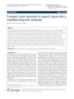
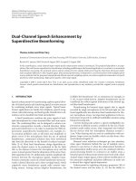
quasi-periodic sound signal (repeat not exactly) is possible. Figure 1 below is an example of
some quasi-periodic signals produced by musical instruments in reality:

Figure 1: Sound signals of some musical instruments

Footer Page 15 of 113.

15


Header Page 16 of 113.
An important kind of periodic signal is sinusoidal signal:
𝑥(𝑡) = 𝐴 sin(2𝜋𝑓𝑡 + 𝜑)
𝐴 is the peak amplitude of signal, 𝑓 is the frequency of signal, and 𝜑 is called the phase.
Sinusoidal signal have a very important property that no other periodic signals have, that is
the sum of two sinusoidal signals with same frequency is another sinusoidal signal with same
frequency:
𝐴1 𝑠𝑖𝑛(2𝜋𝑓𝑡 + 𝜑1 ) + 𝐴2 𝑠𝑖𝑛(2𝜋𝑓𝑡 + 𝜑2 ) = 𝐴3 𝑠𝑖𝑛(2𝜋𝑓𝑡 + 𝜑3 )

The French mathematician Fourier (1768-1830) was the first one who pointed out that any
periodic function can be represented as an infinite sum of sines and cosines functions [4].
That means any periodic signal can be analysed into the sum of many sinusoidal signals. A
periodic signal with frequency 𝑓 will be represented as:
∞

𝑥(𝑡) = ∑(𝑎𝑛 cos(2𝜋𝑛𝑓𝑡) + 𝑏𝑛 sin(2𝜋𝑛𝑓𝑡))
𝑛=0

So a periodic signal with frequency 𝑓 is a sum of sinusoidal signals at frequency
0𝑓, 1𝑓, 2𝑓, 3𝑓, … Thus, the frequency 𝑓 is also called as the fundamental frequency of a
periodic signal.
It is natural to speak about the frequency of periodic signal, but it turns out that aperiodic
signal also has “frequency” too. The mathematicians find out that even aperiodic signal can
be expressed in terms of sinusoidal signals. The discrete sum in the case of periodic signal
becomes the continuous integral in the case of aperiodic signal:
∞

𝑥(𝑡) = ∫ [𝑎(𝑓) cos(2𝜋𝑓𝑡) + 𝑏(𝑓) sin(2𝜋𝑓𝑡)] 𝑑𝑓
0

Therefore, sinusoidal signals can be considered as the basic building blocks of both periodic
and aperiodic signal, just like proton and electron are the building blocks of every atom.
Their difference is that periodic signal is made from a set of sinusoidal signals which have
frequency as an integer multiple of same fundamental frequency, while aperiodic signal does
not have any fundamental frequency.
This theory is named as Fourier analysis, in honour of Joseph Fourier, who was the first
person proposed this theory. Since then, it has important roles in many scientific fields, from
mathematics, physics, acoustics, signal processing, etc.
Frequency of sound signal has an important role in how human perceive sound, which we

will mention in the next section.

Footer Page 16 of 113.

16


Header Page 17 of 113.
2.2. Human perception of sound
It is common fact that human cannot hear some sounds that are audible to some kinds of
animal. Even human adults cannot hear the sounds that the children can hear. The scientists
discovered that normal people can only hear the sounds which have the frequency ranging
from 20 Hz to 20 kHz. It does not mean that human can only hear periodic sounds with
frequency in that range. It means that when a sound signal is decomposed into many
sinusoidal components, only the components with frequency falling in that range is perceived
by human. So, even a periodic sound signal with frequency in 20 Hz to 20 kHz range cannot
be perceived fully by human if it has sinusoidal components at frequency outside of that
range.
Human perception of sound can be divided into three primary characteristics: Loudness, Pitch
and Timbre.

2.2.1. Loudness
Human perception of loudness is mostly depended on the amplitude of sound signal. With the
sinusoidal sound signal:
𝑥(𝑡) = 𝐴 sin(2𝜋𝑓𝑡 + 𝜑)
The higher the value of 𝐴, the louder the sound is. However, the relation between amplitude
and loudness is not linear. That means when the value of 𝐴 increases 𝑛 times, the perceived
loudness does not increase at the same rate. In fact the relation between them is logarithmic.
In practice, we use the Sound Pressure Level (SPL) measure instead of amplitude when
talking about the loudness of sound (the name pressure is used because sound signal is

commonly taken to be the variation of medium’s pressure):
𝑝
𝐿𝑝 = 20 log10 ( ) 𝑑𝐵
𝑝0
𝑝 𝑖𝑠 𝑡ℎ𝑒 𝑟𝑜𝑜𝑡 𝑚𝑒𝑎𝑛 𝑠𝑞𝑢𝑎𝑟𝑒 𝑎𝑚𝑝𝑙𝑖𝑡𝑢𝑑𝑒 (𝑠𝑜𝑢𝑛𝑑 𝑝𝑟𝑒𝑠𝑠𝑢𝑟𝑒)
𝑝0 𝑖𝑠 𝑡ℎ𝑒 𝑟𝑒𝑓𝑒𝑟𝑒𝑛𝑐𝑒 𝑠𝑜𝑢𝑛𝑑 𝑝𝑟𝑒𝑠𝑠𝑢𝑟𝑒
The common chosen sound pressure reference is 𝑝0 = 20 𝜇𝑃𝑎, which is the lowest sound
pressure human can detect (Pa, or Pascal, is the SI unit of pressure). So the lowest level is
defined to be 0 𝑑𝐵, but the highest level is not clearly defined. Normally, the threshold of
feeling is taken to be 120 𝑑𝐵 and the threshold of pain is taken to be 140 𝑑𝐵. Listeners can
detect a change in loudness when 𝐿𝑝 is increased by 1 𝑑𝐵 (which means the amplitude is
multiplied by 101⁄20 ≈ 1.12 times). Acousticians tell us that an increase of 10 𝑑𝐵 (101⁄2 ≈
3.16 times of current amplitude) will give us an impression of double the loudness.
This non-linearity gives human ear an interesting characteristic that it is sensitive to a very
small change in amplitude at low sound pressure level, but is very insensitive to amplitude
change at high sound pressure level.

Footer Page 17 of 113.

17


Header Page 18 of 113.
Aside from amplitude, frequency also has an impact on the perception of loudness. While the
human hearing range is from 20 Hz to 20 kHz, human ear is far more sensitive to the range of
1 kHz to 4 kHz. For example, listeners can detect the 0 𝑑𝐵 𝑆𝑃𝐿 sounds at 3 kHz, while the
sounds at 100 Hz require the sound pressure level of 40 𝑑𝐵 in order to be audible.

2.2.2. Pitch
Pitch is what gives us the impression of “higher” or “lower” sounds. For example, we have a

feeling that female voices are higher than male voices, therefore, we say that the female
voices have higher pitch than the male voices.
The perception of pitch is directly related to the fundamental frequency of a sound signal, so
that we commonly use frequency to measure pitch. However, we must take note that pitch is
a perception, while frequency is a property of objectively existing sound, not depended on
human sensation.
Pitch is directly related to the fundamental frequency, so aperiodic signals without
fundamental frequency do not make any particular pitch. Most musical instruments produce
periodic sounds; only some of them produce aperiodic sounds, like drum or cymbal. Human
ear finds the sounds with fundamental frequency pleasing, while the sounds without any
particular pitch annoying.
Similar to loudness, human perception of pitch is non-linear and logarithmic. Musical pitches
are organized into octaves. The increment of one octave means double the fundamental
frequency. But every octave only consists of 12 different musical notes. That means with the
low pitch sounds, human ear is more sensitive to the change in frequency than with the high
pitch sounds. The below figure of piano keyboard from [5] clarifies that fact:

Figure 2: Musical notes in a piano keyboard

2.2.3. Timbre
Timbre is a complicated perception. With a same musical note, timbre is what helps us know
it is produced by piano, guitar, violin, or human singer. People often say that timbre is
depended on the waveform of sound signal, like in Figure 1, we can see that different musical
instruments produce different sounds waveform. However, this is only partially true. For
example, with the figure below:

Footer Page 18 of 113.

18



Header Page 19 of 113.

Figure 3: Waveform of two particular signals with the same sinusoidal components
combined in a different ways
We can see that the waveforms of both signals are different, but human ear perceives them as
the same sound. This is an interesting fact. Let examined the two above signals more:
𝑥1 (𝑡) = 𝐴1 sin(2𝜋1000𝑡) + 𝐴2 sin(2𝜋3000𝑡)
𝑥2 (𝑡) = 𝐴1 sin(2𝜋1000𝑡) − 𝐴2 sin(2𝜋3000𝑡) = 𝐴1 sin(2𝜋1000𝑡) + 𝐴2 sin(2𝜋3000𝑡 + 𝜋)
It turns out that the only difference between two signals is the phase of 3 𝑘𝐻𝑧 sinusoidal
component. The key of problem is the fact that human ear is sensitive to the amplitude of
each sinusoidal components but very insensitive to the phase of them.
Why the ear is insensitive to phase information? It is because of the fact that sound
propagations of different frequencies are different, so that sounds of different frequencies will
reach the ear through different paths. Therefore, when we change our positions, the phase of
different sinusoidal components will change by different amount, while their amplitude
changes are relatively similar to each other. If human ear is sensitive to phase information,
then we will feel that the sounds are drastically depended on hearing position, even when the
sound sources remain unchanged. This is undesirable, and the natural evolution had proven it
by the phase insensitivity of human ear.

2.3. Audio Signal
2.3.1. Analog audio signal
Before the advent of audio signal, manipulation of sound is not an easy task. It means the
manipulation of the medium of sound. In the late 19th century, Thomas Edison was the first
person who converted sound signal into electrical signal and converted back the electrical
signal into sound. That converted signal from sound is called audio signal. With audio signal,
if we want to manipulate a sound signal, we just need to convert it into electrical audio signal,

Footer Page 19 of 113.


19


Header Page 20 of 113.
let it run through a circuit and convert it back into sound. The audio signal processing field
was born with the advent of audio signal.
The first kind of audio signal was called analog audio signal, because it was analogue to
sound signal. Today, when we talk about analog signal, it often means the signal is
continuous, in contrast with digital signal.

2.3.2. Digital audio signal
Since the advent of digital computer, digital audio signal has gradually replaced the place of
analog audio signal, and nowadays, it is the most common form of audio signal. While the
range and domain of analog signal are continuous, the range and domain of digital signal are
discrete. While the usage of digital signal lead to inevitable information loss from analog
signal, it has the advantage that we can apply exact manipulation on them. Analog signal on
the other hand, is harder to manipulate because of physical constraints and noises during
processing and transmission.
The converting process from analog signal to digital signal is called sampling and
quantization.

2.3.3. Sampling
Sampling is the process that converts the continuous domain of analog signal into a discrete
domain. It means that a continuous signal is converted into a discrete series of values. The
ratio of conversion is called sampling rate. If a one second analog signal is converted into a
series of 100 values, then the sampling rate is 100 Hz (it has the same unit as frequency). For
example, Figure 4 below shows a sine wave signal and the result signal after sampling:

Figure 4: Sampling of a sinusoidal analog signal


Footer Page 20 of 113.

20


Header Page 21 of 113.
The above case is an example of proper sampling. Because there is only one sine wave (with
frequency not lower than the original signal) that can match with the sampled signal,
therefore we can reconstruct the original analog signal from the sampled signal. However, not
all sampling processes are proper. For example:

Figure 5: Sampling process with low sampling rate
In this case, the sampling rate is lower than the frequency of sinusoidal signal. As we can see
from the Figure 5, there is another sinusoidal signal that matches with the sampled signal.
Therefore, we cannot restore the original signal from the sampled signal. As a general rule,
the higher the sampling rate, the better. But depend on the actual application; we only need a
particular high sampling rate. For example, the sampling rate in Figure 4 is high enough; we
do not need a higher sampling rate.
The Nyquist-Shannon sampling theorem indicates that if a signal x(t) is sampled at regular
intervals of time and at a rate higher than twice the highest signal frequency, then the samples
contain all the information of the original signal. The signal x(t) may be reconstructed from
these samples by the use of a low-pass filter. With this theorem, we can know how much high
the sampling rate should be. [5]
For audio signal, there are two common sampling rates: 8000 Hz and 44100 Hz. Note that
they are corresponding to the most sensitive range of hearing (4000 Hz) and human limit of
hearing (20000 Hz). [5]

Footer Page 21 of 113.


21


Header Page 22 of 113.
2.3.4. Quantization
The signal after sampling is only discrete-time signal, not digital one. Because the digital
computer can only work with discrete values, we must do another step to convert the
continuous range of discrete-time signal into discrete range. That step is called quantization.
Contrast to sampling, where we can preserve perfectly any sinusoidal components with
frequency lower than half sampling rate, quantization error cannot be removed entirely,
because we cannot expect every amplitude value at sample points is falling exactly into our
discrete range. Quantization error is also called as quantization noise because of its random
nature.
For example, we use a 16 bit integer to represent the amplitude of a signal. That means our
discrete range will contain 65536 equally spaced values. The maximum quantization error at
one sample is not greater than ± 1⁄2 𝐿𝑆𝐵. LSB is least significant bit, which means the
amplitude value represented by one least significant bit. It also is the amplitude distance
between adjacent quantization levels. The quantization error at a sample can be considered a
random variable uniformly distributed over ± 1⁄2 𝐿𝑆𝐵. Therefore, the total quantization error
can be thought as an additive noise and quantization is the process that adds this noise into
the discrete-time signal.
This model is very powerful, because the quantization noise is just added into whatever noise
has already existed in the original signal. If the existing noise is high compare to quantization
noise, then the presence of quantization noise will be insignificant. Thus, we only need to
increase the quantization resolution until the quantization noise is smaller than existing noise.

2.4. Fourier Transform and Frequency domain representation
Normally, the audio signal is represented as a function of time. However, this form of
representation sometime is hard to work with. For example, we want to increase the
amplitude of the 1 𝑘𝐻𝑧 sinusoidal component of one particular audio signal 𝑥(𝑡). It is very

complicated to calculate directly with 𝑥(𝑡). A wise method would be decomposing 𝑥(𝑡) into
sinusoidal component, modifying on each component, and then synthesizing them back
into 𝑥(𝑡). That is the basis of Fourier Transform and frequency domain representation.
With a signal represented as a function of time:
𝑥(𝑡)
Decompose it into sinusoidal components:
∞

𝑥(𝑡) = ∫ [𝑎(𝑓) cos(2𝜋𝑓𝑡) + 𝑏(𝑓) sin(2𝜋𝑓𝑡)] 𝑑𝑓
0

With the Euler rule: 𝑒 𝑖𝑥 = cos 𝑥 + 𝑖 sin 𝑥, we will have:

Footer Page 22 of 113.

22


Header Page 23 of 113.
𝑒 𝑖2𝜋𝑓𝑡 + 𝑒 −𝑖2𝜋𝑓𝑡
cos(2𝜋𝑓𝑡) =
2
sin(2𝜋𝑓𝑡) =
∞

𝑥(𝑡) = ∫ (𝑎(𝑓)
0

𝑒 𝑖2𝜋𝑓𝑡 − 𝑒 −𝑖2𝜋𝑓𝑡
2𝑖


𝑒 𝑖2𝜋𝑓𝑡 + 𝑒 −𝑖2𝜋𝑓𝑡
𝑒 𝑖2𝜋𝑓𝑡 − 𝑒 −𝑖2𝜋𝑓𝑡
+ 𝑏(𝑓)
) 𝑑𝑓
2
2𝑖
∞

= ∫ ((
0

𝑎(𝑓) 𝑏(𝑓) 𝑖2𝜋𝑓𝑡
𝑎(𝑓) 𝑏(𝑓) −𝑖2𝜋𝑓𝑡
+
)𝑒
+(
−
)𝑒
) 𝑑𝑓
2
2𝑖
2
2𝑖

The integral above can be rewritten as:
∞

𝑥(𝑡) = ∫ 𝑐(𝑓) 𝑒 𝑖2𝜋𝑓𝑡 𝑑𝑓
−∞


𝑐(𝑓) = {

0.5𝑎(𝑓) + 0.5𝑖𝑏(𝑓),
0.5𝑎(𝑓) − 0.5𝑖𝑏(𝑓),

𝑓>0
𝑓≤0

In the field of signal processing, the Fourier Transform is used to transform a signal in time
domain (function of time) into a signal in frequency domain (function of signal). The
transformed signal is denoted as 𝑋(𝑓):
𝑥(𝑡) : − ∞ < 𝑡 < ∞
𝑋(𝑓) : − ∞ < 𝑓 < ∞
𝑋(𝑓) = 𝑐(𝑓)
∞

𝑥(𝑡) = ∫ 𝑐(𝑓) 𝑒 𝑖2𝜋𝑓𝑡 𝑑𝑓
−∞

The question is how to calculate 𝑐(𝑓). The mathematicians had determined that:
∞

𝑐(𝑓) = ∫ 𝑥(𝑡)𝑒 −𝑖2𝜋𝑓𝑡 𝑑𝑡
−∞

Thus, the Fourier Transform equations are:
∞

𝑋(𝑓) = ∫ 𝑥(𝑡)𝑒 −𝑖2𝜋𝑓𝑡 𝑑𝑡

−∞
∞

𝑥(𝑡) = ∫ 𝑋(𝑓) 𝑒 𝑖2𝜋𝑓𝑡 𝑑𝑓
−∞

The first equation is the forward transform (from the time domain to frequency domain), the
second one is inverse transform (from the frequency domain to time domain).
Note that the transformed signal 𝑋(𝑓) is complex signal and not real signal.

Footer Page 23 of 113.

23


Header Page 24 of 113.
In signal processing term, we call 𝑋(𝑓) is the frequency spectrum of audio signal 𝑥(𝑡). The
value of 𝑋(𝑓) characterize both the amplitude and phase of the sinusoidal component with
frequency 𝑓.
When we represent the complex value 𝑋(𝑓) in polar form, its absolute value is the amplitude
of sinusoidal component; its argument is the phase of sinusoidal component. Therefore, we
also call |𝑋(𝑓)| the magnitude spectrum and ∠𝑋(𝑓) the phase spectrum. The frequency
spectrum can be considered as the combination of magnitude and phase spectrum. The
benefit of those two spectrums is that they are real signal, not complex, so it is more
convenient to work with them.
The above is only the Fourier transform for aperiodic continuous signals, for other kind of
signals, the Fourier Transform is different: [6]
Table 1: Different kinds of signal and their Fourier Transforms
Signals


Fourier Transform
𝑥(𝑡): 0 ≤ 𝑡 ≤ 𝑇
𝑋[𝑘]: … , −2, −1, 0, 1, 2, …
𝑇

1
𝑋[𝑘] = ∫ 𝑥(𝑡)𝑒 −𝑖2𝜋𝑘𝑓𝑡 𝑑𝑡
𝑇

Periodic continuous with
fundamental frequency 𝑓 and
fundamental period 𝑇

0

∞

𝑥(𝑡) = ∑ 𝑋[𝑘]𝑒 𝑖2𝜋𝑘𝑓𝑡
𝑘=−∞

𝑥[𝑛]: … , −2, −1, 0, 1, 2, …
𝑋(𝜔): −𝜋 ≤ 𝑓 ≤ 𝜋
∞

𝑋(𝜔) = ∑ 𝑥[𝑛]𝑒 −𝑖𝜔𝑛

Aperiodic discrete

𝑛=−∞
𝜋


𝑥[𝑛] =

1
∫ 𝑋(𝜔) 𝑒 𝑖𝜔𝑡 𝑑𝜔
2𝜋
−𝜋

𝑥[𝑛]: 0, 1, … , 𝑁 − 1
𝑋[𝑘]: 0, 1, … , 𝑁 − 1
𝑁−1

1
𝑋[𝑘] = ∑ 𝑥[𝑛]𝑒 −𝑖𝜔𝑛
𝑁

Periodic discrete with period 𝑁,
radian frequency 𝜔

𝑛=0

𝑁−1

𝑥[𝑛] = ∑ 𝑋[𝑘]𝑒 𝑖𝜔𝑛
𝑛=0

Footer Page 24 of 113.

24



Header Page 25 of 113.
2.5. Kalman Filter
In reality, we often need to measure some quantities, but the measurements will inevitably
contain some noises and not equal to the quantity we need to determine. Hence, it is always
desirable to reduce the influence of the noise to the measurement values. However, in the
case we cannot reduce the noise anymore; we will want to estimate what is the most probable
value for a quantity, given its measurement. Kalman Filter is one of the methods to do that
job.
Kalman Filter is the algorithms that operated recursively on the stream of noisy measurement
to estimate the statistical optimal value of the underlying system state. It assumes the system
state is changing as a linear process, and the noise is Gaussian white noise. The model is
formally described as below: [7]
𝑥𝑛 = 𝐴𝑛 𝑥𝑛−1 + 𝐵𝑛 𝑢𝑛 + 𝑤𝑛
𝑧𝑛 = 𝐻𝑛 𝑥𝑛 + 𝑣𝑛
𝑥𝑛 is the underlying system state at time 𝑛, 𝑢𝑛 is the control input signal, 𝑤𝑛 is the process
noise, 𝑧𝑛 is the measurement value, 𝑣𝑛 is the measurement noise. In general case, they are all
vectors. 𝐴𝑛 , 𝐵𝑛 , 𝐻𝑛 are called transformation matrices.
𝑤𝑛 , 𝑣𝑛 are assumed to be Gaussian white noises. The covariance matrix of 𝑤𝑛 is 𝑄𝑛 , and the
covariance matrix of 𝑣𝑛 is 𝑅𝑛 .
The Kalman Filter algorithm is performed recursively in two steps: [7]
Prediction step:
The prediction value of 𝑥𝑛 from past estimation 𝑥̂𝑛−1|𝑛−1 is calculated:
𝑥̂𝑛|𝑛−1 = 𝐴𝑛 𝑥̂𝑛−1|𝑛−1 + 𝐵𝑛 𝑢𝑛
The covariance of this prediction is:
𝑃𝑛|𝑛−1 = 𝐴𝑛 𝑃𝑛−1|𝑛−1 𝐴𝑇𝑛 + 𝑄𝑛
Update step:
The Kalman gain is calculated:
𝐾𝑛 = 𝑃𝑛|𝑛−1 𝐻𝑛𝑇 (𝐻𝑛 𝑃𝑛|𝑛−1 𝐻𝑛𝑇 + 𝑅𝑛 )


−1

The updated estimation of 𝑥𝑛 is calculated as:
𝑥̂𝑛|𝑛 = 𝑥̂𝑛|𝑛−1 + 𝐾𝑛 (𝑧𝑛 − 𝐻𝑛 𝑥̂𝑛|𝑛−1 )
The covariance of this estimation is:
𝑃𝑛|𝑛 = (𝐼 − 𝐾𝑛 𝐻𝑛 )𝑃𝑛|𝑛−1

Footer Page 25 of 113.

25