JM02007 vibration principles
Bạn đang xem bản rút gọn của tài liệu. Xem và tải ngay bản đầy đủ của tài liệu tại đây (1.23 MB, 32 trang )
Ref. FK4KZ5GIe
Vibration Principles
An Introduction to Spectrum Analysis
Summary
One of the most important tools used in the investigation of
bearing vibration is frequency spectrum analysis. Therefore, it is
important that technicians and managers understand the
possibilities and limitations of this technique. This document
explains in detail, displacement, velocity, and acceleration, and
the methods used to obtain these measurements. Also included is
the derivation of a frequency spectrum by Fourier transform, the
consequences of sampling, and the value found in finite
measurements.
Franz Reithuber
SKF Quality Technology Center
32 pages
1992
SKF Reliability Systems
@ptitudeXchange
4141 Ruffin Road
San Diego, CA 92123
United States
tel. +1 858 244 2540
fax +1 858 244 2555
email:
Internet: www.aptitudexchange.com
Use of this document is governed by the terms
and conditions contained in @ptitudeXchange.
Licenced to SKF Vietnam/Tran Hong Doan. Downloaded on Feb 5, 2004
Ref. FK4KZ5GIe
Document Title
Introduction
One of the most important tools used in the
investigation of bearing vibration is frequency
spectrum analysis. Therefore, it is important
that technicians and managers understand the
possibilities and limitations of this technique.
This document explains in detail,
displacement, velocity, and acceleration, and
the methods used to obtain these
measurements. Also included is the derivation
of a frequency spectrum by Fourier transform,
the consequences of sampling, and the value
found in finite measurements.
Understanding the methods and processes
behind the use of a particular tool can greatly
increase the effectiveness of that tool. This is
especially the case of spectrum analysis,
where the 'mystic flair' is transformed into a
well-understood, simple process. The ability
to clearly convey how this process is achieved
lends a great amount of respect to person and
company.
mathematicians use ‘y’ for the ordinate and
‘x’ for the abscissa (Figure 1).
Figure 1. A function Represented in a Cartesian grid.
We can say 'y' is a function of 'x' and write it
as:
y = f (x)
(1)
For each point of 'x' for which the function
exists, a corresponding point on 'y' can be
found; thus, 'y' is a projection of 'x'.
One of the simplest mathematical functions is
a straight line:
Spectrum analysis of displacement, velocity,
and acceleration measurements allows one to
better understand what is occurring in the
system. These three measurement types are
the physical domains in which we can
describe static and dynamic situations.
Therefore, a basic understanding of
measurement parameters is necessary. Here
we begin with the basic terminology.
y=kx+d
(2)
What is a Function?
When one thing is dependant upon another,
and there is a correlation between the two
items, the relationship can possibly be
expressed in a graph or formula. This
graphical form is referred to as a function.
The most common graph is the Cartesian grid.
Two axes are drawn at right angles. The
vertical axis is called ordinate (y), and the
horizontal axis is the abscissa (x). In general,
Figure 2. Straight Line as a Function.
In Figure 2, 'd' represents the initial
displacement on the ordinate and 'k' indicates
the slope of the line. When 'k' equals one and
'd' is zero, we get a 45-degree line through the
zero-point of the grid (the scale of the axes is
must be the same). Equation (2) describes a
straight line exactly in an infinite twodimensional space.
© 2002 SKF Reliability Systems All Rights Reserved
Licenced to SKF Vietnam/Tran Hong Doan. Downloaded on Feb 5, 2004
2
Ref. FK4KZ5GIe
Document Title
What is a Sine Wave?
A sine wave is a special function of
tremendous importance in the investigation of
vibration.
According to equation (3), a sine wave can be
written as a function:
y = A sin (x)
(3)
The projection on our ordinate depends on a
constant factor 'A' (amplitude), which is
multiplied by the sine-function, where 'x' is an
argument indicated by brackets. Any
calculator, table, or slide rule gives us the
right value when we put in the argument 'x'.
But, what is the foundation behind this?
You may have seen ‘π’ in connection with
sine-functions. Remember, the circumference
of a circle with diameter one equals π. When
we describe a circle by its radius we get 2π as
the circumference when the radius is one. This
example indicates that a sine wave is
somehow connected to a circle. Actually, a
sine wave is a projection of a point on a circle,
as it is a function over the angle.
the radius; therefore, it is a function of the
angle.
On the abscissa we can draw the angles and
their corresponding borderline between bright
and dark. The curve from this is a sine wave.
In principle, a cosine wave is the same, with
its phase shifted 90 degrees. At the zero-point
of the coordinates the cosine-wave starts at the
positive maximum.
It becomes obvious, therefore, that a function
so strongly connected to rotation is important
for describing bearing behavior.
Physical Domains
There are different types of transducer that can
be used for the three physical domains of
displacement, velocity, and acceleration.
Based on their specific principle of operation,
their response is proportional to the physical
domain (Figure 4).
Figure 3. Generation of a Sine Wave.
Let’s assume we have a radius 'r' rotating
counter-clockwise (Figure 3). Parallel lightrays come from the left side and generate a
bright and a dark field at the projection
surface 'y'. The borderline between dark and
bright moves up and down according to the
rotation of the radius. The current position of
the borderline depends on the current angle of
Figure 4. Three Major Types of Transducers.
Deciding which sensor principle to use
depends on the performance of the measuring
© 2002 SKF Reliability Systems All Rights Reserved
Licenced to SKF Vietnam/Tran Hong Doan. Downloaded on Feb 5, 2004
3
Ref. FK4KZ5GIe
Document Title
principles in the existing frequency range, and
the parameters you are seeking.
driver traveled. The result of this division is an
indication of the speed υ:
Displacement
According to Figure 5, displacement tells us
the distance between two points, measured in
millimeter or inches.
The words distance and displacement are, in
principle, describing the same type
measurement; however, ‘distance’ describes
static situations like diameters or lengths
between two points.
υ=
s
t
(4)
To normalize the result for comparison
reasons, we agree upon measurement units.
When the speedometer in a European car
displays 100 km per hour, a European citizen
realizes the meaning according to the map. An
American citizen expresses the value in miles
per hour to understand how long it takes to
arrive at the destination. Normally, neither
drivers recognize the importance of speed in
relation to unexpected events. Apart from
speed limits, nobody drives 100 km/h in an
urban area where children are playing because
each second his car moves 28 meters. This is
an example of choosing units to transmit the
necessary message.
The result of the equation (4) is an average
value that does not tell us the speed in
different parts of the route. To reach that
information we can divide the route into
different parts indicated by delta (∆). Thus,
the distance between Madrid and Toulouse is
∆s, and the driving time: ∆t. This results in a
new velocity:
υ=
Figure 5. Example of Displacement (Y) and Distance (X).
The word ‘displacement’ describes the
deviations around a middle value, measured in
a unit of distance. The most common
displacement units when judging the quality
of bearing components are:
µm or µinch
Velocity
When we ask how fast somebody drove from
Madrid to Gothenburg, we divide the distance
's' between the two towns, by the time 't' the
∆s
∆t
(5)
Since this is still an average velocity, we do
not know if the driver exceeded the maximum
speed. We can solve this problem by dividing
the route into smaller parts. However, how
small should ∆s be? Taking into account that
the car cannot accelerate infinitely fast, we
find some suitable values for ∆s, but we will
never be exact. When we want to know the
speed of the car at each point of the route
exactly, we have to reduce ∆s to an infinitely
small distance. This means that the route
consists of an infinite number of different
parts, independent of the length of the route.
© 2002 SKF Reliability Systems All Rights Reserved
Licenced to SKF Vietnam/Tran Hong Doan. Downloaded on Feb 5, 2004
4
Ref. FK4KZ5GIe
Document Title
Mathematically we have to cross the border to
the so-called “infinitesimal calculus,” which
sounds more complex than it is. Based upon
the rules of calculus we can change equation
(5) to:
υ=
∂s
∂t
(6)
∆ is now written as a ‘∂’, thus the equation is
‘∂s over ∂t’. Another way to express it is to
say, "distance s is differentiated over time t.”
When we referred to Figure 3, we let the
radius rotate to explain how a sine wave is
generated. Now we can also ask how fast our
radius is rotating. As we did for distances, we
can define an angular speed by dividing a
certain distance by a special time-unit.
After one rotation the same situations repeats
itself, which allows us to choose one rotation
as a distance-unit. Since we are looking for
angular speed, we can make life easier by
choosing the radius-unit one. Therefore, our
distance-unit becomes 2. The symbol ω
(omega) is used to describe angular speed:
ω=
2π
T
ω=2πf
(9)
When we multiply ‘ω’ (angular speed) by time
‘t’, we come back to angle ‘φ’.
Mathematically, T and t cancel each other out:
φ=ωt=
2π
t=2π
T
(10)
when t = T
In equation (3) we expressed 'x' as an abstract
argument for our sine wave. In Figure 3 the
abscissa is also called 'x', but scaled in ‘φ’.
According to our example we can now be
more precise and name the abscissa as an
angle. Time is always an important parameter
when studying technical problems. To
emphasize this, the abscissa’s name changes
from ‘φ’ to ‘ωt’.
(7)
The time-unit 'T' is called periodic time. If the
periodic time is one second, we have one
rotation per second. In the case of 0.5 seconds
periodic time, we have two rotations per
second (one rotation is repeated twice in our
time-unit). We can also say our rotation is
twice as frequent as our first example, which
brings us to the word ‘frequency’ (f).
Frequency is measured in Hertz (Hz). From
our example we can derive the relation
between periodic time and frequency:
1
f=
T
The equation for ω can now be written as:
(8)
Figure 6. Representation of Replacing ωt at the
Abscissa to Arrive at Equation (11).
Equation (3) can now be written as:
y = A sin (ωt)
(11)
The amplitude 'A' can be the radius of our
circle, in part or multiple.
Now we have the basics to analyze the
consequences of the differential equation (6).
There are some special rules of differential
equations that are not be covered in this
discussion. Instead, we focus only on the
simplest ones.
© 2002 SKF Reliability Systems All Rights Reserved
Licenced to SKF Vietnam/Tran Hong Doan. Downloaded on Feb 5, 2004
5
Ref. FK4KZ5GIe
Document Title
In simple terms, the first derivation of a
function tells us the slope of the function at
each point. From equation (6), it is obvious
that velocity is zero when there is no deviation
‘n’, distance, which means the driver stands
still.
Refer to equation (2) and Figure 2, where we
abstractly defined the function of a straight
line. We can apply this straight line to our
driver when we assume he drove for a time at
a constant speed. Then we can name the
abscissa time and scale it in hours. On the
ordinate, draw the meter indication (km) of
the odometer in the car. The constant 'd' in
equation (2) becomes the meter indication at
the beginning of our observation (km (start)).
We can now write equation (2) applied to this
example as:
km = kt + km (start)
(12)
In equation (12) 'k' is the most important
factor when looking for the speed of a car.
When 'k' is zero, 'km' does not increase, which
means the car stands still. The greater 'k', the
faster our meter counts, and the faster the car.
Thus, factor 'k' is the speed of the car.
In equation (6) we saw that velocity is derived
from displacement, or distance over time.
Using the common parameters, equation (12)
appears as:
s = kt + s0
(13)
s0 is the constant factor and indicates the
position at the beginning of observation.
To make life easier there is an international
convention: derivations over time 't' can be
expressed by an apostrophe after, or a point
over, the variable in question:
υ=
∂s
= s’
∂t
(15)
Following the same rules, angular speed ‘ω’
can be expressed as the derivation of the angle
(φ or ωt) over time, written as φ’ or ∂φ/∂t:
φ’ =
∂
(ωt) = ω
∂t
(16)
The factor at the variable where we apply the
derivational process is the proper result.
But, what happens if our displacement follows
a sinusoidal function? Let’s replace the
abstract name 'y' in equation (11) by
displacement 's':
s = A sin (ωt)
(17)
Which vertical velocity ‘v’ do we get?
Assume we have a sinusoidal road and we
drive on this road with constant horizontal
speed as shown in Figure 7. At the top and the
bottom of our road we do no have any vertical
velocity. The maximum value of vertical
velocity is at the sinusoidal road’s points of
highest slope. These points are obviously
where the sine wave of the road crosses the
abscissa.
Based on our example we know that:
υ=
∂s
∂
=
(k t + s0) = k
∂t
∂t
(14)
The constant factor s0 no longer exists. The
factor multiplying the variable 't' (to which we
apply the derivational process) is our desired
result.
Figure 7. Representative of Displacement (Black), and
Vertical Velocity (Red).
© 2002 SKF Reliability Systems All Rights Reserved
Licenced to SKF Vietnam/Tran Hong Doan. Downloaded on Feb 5, 2004
6
Ref. FK4KZ5GIe
Document Title
When we also analyze the situation outside the
extreme points, we find the wave for vertical
velocity (Figure 7). Once again, this is a sine
wave shifted through 90 degrees. As
previously mentioned, we call such a function
a cosine wave.
Now that we know the derivation of a sine
wave is a cosine-wave, we have found a
general rule. But, before we derive equation
(17) we must take into account that the
argument of the sine wave is ωt, which itself
has to be derived. This is called the inner
derivation. We saw previously that the result
is ω. Based on the fact that the function is
linear, we can combine the results of the inner
and the outer derivation via multiplication,
and come to the desired result for the vertical
velocity:
υ=
∂s
= ω A cos (ωt)
∂t
(18)
The result of the inner derivation ω, becomes
a multiplication-factor. This is very important
for the relation between displacement and
velocity. Since ω equals 2πf, the frequency is
involved in the answer. It can be shown that
the higher the frequency of the sinusoidal
road, the higher the resulting vertical velocity.
This fact can easily be demonstrated with an
experiment. Assume two wagons are pulled
with the same horizontal speed over two types
of roads (Figure 8).
Figure 8. Example of Two Types of Velocities.
Though the road with the higher frequency has
lower amplitude, passengers pulled over this
road have much more trouble.
This example shows that frequency has a
tremendous importance for responses in the
different physical domains. For example,
waves on rings or rollers may cause big
quality problems in the application, even if the
displacement proportional amplitude is below
the diameter of an atom!
The most common units in measuring velocity
to judge bearing quality are:
µm/s or µinch/s
Acceleration
In principle we have the same relation
between acceleration and velocity as between
velocity and displacement. Acceleration
answers the question: how fast does velocity
change? Therefore, it describes the slope of
the velocity function. The same rules we
found when discussing velocity can be applied
to acceleration. To derive acceleration from
velocity the following equation has to be used:
a=
∂ν
∂b
© 2002 SKF Reliability Systems All Rights Reserved
Licenced to SKF Vietnam/Tran Hong Doan. Downloaded on Feb 5, 2004
(19)
7
Ref. FK4KZ5GIe
Document Title
Since the velocity ‘v’ is derived from
displacement 's', acceleration is the second
order differentiation of displacement. This is
conventionally indicated in a formula as:
a=
∂2s
∂t 2
(20)
If we assume we have a velocity following a
sine wave function, we just replace ‘v’ by ‘a’,
and ‘s’ by ‘v’ in equation (18) to derive the
acceleration. The velocity is multiplied by ω,
and once again we have the frequency
dependence in the acceleration proportional
response. The higher the frequency, the higher
the acceleration even at the same velocity
level.
When we want to derive acceleration from
displacement, we apply the derivational
process to equation (18). From the inner
derivation of ωt, we get additional
multiplication with ω and end up with ω2.
Following the same rules we used in Figure 7
to derive velocity from displacement, we find
the slope of a cosine wave as an inverse sine
wave. Therefore, we arrive at:
a=
∂2s
= -ω A sin (ωt)
∂t 2
Vibration
We just discussed the three physical domains
in which we can measure, and the difference
between distance and displacement.
The deviation surrounding a middle value is
typical of vibration, regardless of the physical
domain. This deviation represents a wave that
can be transmitted through solids via
transverse or longitudinal waves, and hits our
ears as a sound pressure wave.
The physical domain selected for measuring
depends only on the considered parameters
and the performance of the sensor system in
the desired frequency area.
Figure 9 lists common sensor-systems and
describes the principle of operation.
(21)
Acceleration is very important for dynamic
mechanics because force is connected with
acceleration in the Newton equation:
F=ma
(22)
In this equation 'm' indicates mass, which is
normally measured in kg.
The most common acceleration units of
measurement are:
m/s2 or inch/ s2
Figure 9. The Principle Properties of Sensors in the
Three Physical Domains.
The following explanation only gives an
impression of the principle of operation. For
more details please refer to basic literature
about measuring techniques. However, it is
not necessary to understand sensors in detail
to achieve good results.
© 2002 SKF Reliability Systems All Rights Reserved
Licenced to SKF Vietnam/Tran Hong Doan. Downloaded on Feb 5, 2004
8
Ref. FK4KZ5GIe
Document Title
LVDTs
Linear Variable Displacement Transducers
(LVDTs) are common for measuring
displacement. A differential coil-system is
connected to a precise sine wave generator. A
magnetic cylinder connected to the tip
influences the impedances of the coils.
Therefore, the impedance ratio is a function of
the sensor’s position. Since the impedance
ratio is responsible for the distribution of the
bridge sine wave, the amplitude of the outputvoltage is also directly related to the position
of the sensor. A simple rectifier or a more
advanced enveloping demodulator can prepare
the signal for further processes. Common
bridge frequencies are between 5 kHz and 20
kHz.
Moving Coils
The principle used in moving coil transducers
has been understood since the beginning of
electrical techniques in generators and electric
motors. Broadcasting stations continue to use
this concept in microphones. The principle
shows that whenever a wire is moved in a
magnetic field (or the magnetic field changes
in time) a voltage is induced in that wire. The
amplitude of this voltage depends upon the
strength of the magnetic field and the length
of the wire (coil). When all other parameters
are constant, the voltage generated in this kind
of sensor is proportional to the speed of the
coil. Since the coil, in the case of a moving
coil transducer is connected to the tip, we
measure velocities with these sensors.
Piezoelectric Transducers
In some crystals, charge can be drained away
when pressure is applied. The effect results
from special triangular structures of the
molecules. For measuring acceleration, this
type of transducer is based on the seismic
principle. One side of the crystal is connected
to the object, and on the other side a mass is
mounted without a connection to the sensor
housing. According to equation (22) a force is
applied to the crystal when the transducer is
accelerated. This force generates a charge that
is transferred into voltage in a capacitor. Since
the mass is constant when we are far enough
below the speed of light, the voltage we
measure is proportional to acceleration.
Now we can ask the question, which sensorsystem should be used for noise problems?
Before we can give an answer, we have to be
more precise. Do we want to judge the quality
in an application, do we want to select the
bearings after final assembly, or do we want to
check the quality of the individual bearing
parts?
Based on the equations we previously derived,
we can draw a graph (Figure 10).
Figure 10. Frequency Response of Displacement
(Blue), Acceleration (Yellow) Based Upon Constant
Velocity (Red). The Two Vertical Lines on the Graph
are Referenced as f1 and f2.
If we assume we have constant velocity over
the whole frequency range, the displacement
proportional and the acceleration proportional
response are totally different. In figure 10,
assume the first vertical line on the graph is f1
the second is f2, and where displacement and
acceleration responses intersect is velocity.
Where the frequencies f1 and f2 are really
located depends on the sensitivities of the
sensor systems.
Below f1, displacement should be used
whenever it is possible. Velocity is a
© 2002 SKF Reliability Systems All Rights Reserved
Licenced to SKF Vietnam/Tran Hong Doan. Downloaded on Feb 5, 2004
9
Ref. FK4KZ5GIe
Document Title
compromise, but acceleration is the totally
wrong decision. There is a frequency band
between f1 and f2 where velocity represents
the best solution, and displacement or
acceleration can be an alternative. Frequencies
higher than f2 require acceleration as the
proper physical domain, and nobody
displacement should not be used in this area.
Therefore, for quality assessment of bearings
we have displacement proportional and
velocity proportional equipment for roundness
and waviness testing of individual bearing
parts. To judge the noise of assembled
bearings, velocity proportional measuring
equipment is in common use. The procedure is
laid down in a standard. According to this
standard, the bearing has to run at 1800 RPM,
and velocity proportional RMS-values must be
measured in three filter bands (band A: 50
Hz–300 Hz, band B: 300 Hz-1800 Hz, band
C: 1800 Hz–10,000 Hz). Some producers use
acceleration for this purpose regardless of the
international standards, and they also come up
with good quality results.
To monitor a bearing in its application, the
monitoring equipment has to respond to pulses
caused by a bearing defect. Since the
frequency response on pulses goes up to very
high frequencies, acceleration proportional
monitoring equipment is usually used for this
purpose.
There is an additional argument to assess the
noise of assembled bearing’s velocityproportionally. According to Figure 11, our
sound impression is proportional to the
velocity of a vibrating surface. Therefore, it
makes sense to select the same physical
domain in which the customer will judge the
noise level of a bearing.
Figure 11. The Human Sound Impression.
Why Spectra?
It is somewhat common to describe certain
parameters in relationship to other parameters.
For example, we often describe speed in miles
or kilometers per hour. Angles and certain
other parameters are also addressed as
functions of time or time domain functions.
Time domain functions are very useful tools
that describe a great deal of information.
However, when we use time domain functions
sometimes we don’t receive the required
information. For example, when looking for
the frequency content of a signal, the time
domain may only help us at the dominant
frequencies, but often the needed information
is at a less dominant frequency.
Let us give some examples. When we make a
roundness measurement of an eccentric oval
as shown in Figure 12, the sensor generates
the signal in the linear chart.
© 2002 SKF Reliability Systems All Rights Reserved
Licenced to SKF Vietnam/Tran Hong Doan. Downloaded on Feb 5, 2004
10
Ref. FK4KZ5GIe
Document Title
Figure 12. Roundness Measurement of an Eccentric Oval.
Without any further information beside the
linear chart we could say that the result is
dominated by eccentricity, but influenced by
some other parameter.
In our experiment we can project the vector of
eccentricity alone as we did during the
discussion of how a sine wave is generated.
Drawn over the angle we get a pure sine wave
within one rotation: the response of
eccentricity. This result is described as the
first order, as it has only one positive and one
negative part.
When we assume we have only ovality
without eccentricity, the sensor is moved
twice up and twice down during one rotation.
We can then say ovality is of the second order,
which means that two positive and the
negative parts are present during one rotation.
We can draw a representative vector of ovality
by rotating twice as fast as the vector of
eccentricity. The projection of this vector over
the angle is the response of ovality.
In Figure 12 it is apparent that the ovality of
the measured part does not coincide with
eccentricity. The orientation of ovality is 22.5
degrees in front of eccentricity; that is, the
sine wave for ovality starts with a phase-shift
of 22.5 degrees or π .
8
When we add the values of the two sine waves
we have from our projection at each anglepoint, the result is a curve in the linear chart.
Therefore, the individual waves tell us the
content of pure sine waves in the linear chart.
Since the linear chart represents the signal we
received from the sensor, we can never ask
directly for the content of pure sine waves.
But, the answer to this question becomes more
and more interesting when investigating puretone problems.
© 2002 SKF Reliability Systems All Rights Reserved
Licenced to SKF Vietnam/Tran Hong Doan. Downloaded on Feb 5, 2004
11
Ref. FK4KZ5GIe
Document Title
To display the sine wave content of the linear
chart on another chart, the so-called frequency
chart or spectrum is much more convenient,
especially when a lot of individual sine waves
are present. For example, with outer rings we
have to take into account 923 individual sine
waves. If this were the case, the result would
be nothing but a black bar in our time domain
chart.
the amplified signal received from a
microphone on a digital storage oscilloscope
(Figure 14). The time signals are different, but
which is the vocal ‘A’ and which the vocal
‘E’?
The ordinate keeps the unit, in our case
displacement, but the unit at the abscissa
changes from angle to order number. We call
the lines at the order numbers harmonics.
When the linear chart depends upon time, the
spectra depend upon frequency. Since this is
the most common case, we call the spectra
'frequency domain' or ‘frequency chart', even
when the abscissa is not marked in frequency
units.
For our simple example we can draw a
spectrum (Figure 13). In this example, only
the first and second order numbers exist.
Figure 14. Time Signal of Vocal ‘A’ and Vocal ‘E’.
Figure 13. Spectrum for the Example in Figure 12.
In order to answer this question we should
look at the frequency domain as shown in
Figure 15. Instead of time at the abscissa we
have frequency, and the ordinate is marked in
voltage as before. To make the response more
understandable a logarithmic scale in decibels
(dB) is used. This type of scaling also makes
lower amplitudes visible that would be hidden
in a linear scale. The rule for calculating the
logarithmic scale in our example is: (0dB = 5
Volt)
Order number zero represents the offset of the
sensor from its electrical zero point. This
offers the possibility of measuring also
diameters related to a master part. In an
electrical signal the value of the zero harmonic
tells the DC-content (direct current).
In the next example let’s analyze the voice of
a vocalist. Two vocals ‘A’ and ‘E’ are sung at
the concert pitch ‘a’ (440 Hz). First we display
When we measure the time between two peaks
of the first chart we find a distance of 6.8
milliseconds. The corresponding frequency (f
= 1/t) is 147 Hz, which is only a third of the
desired concert pitch frequency. Has our
vocalist made a mistake?
amplitude
response[dB] = 20 log
5 Volts
© 2002 SKF Reliability Systems All Rights Reserved
Licenced to SKF Vietnam/Tran Hong Doan. Downloaded on Feb 5, 2004
(23)
12
Ref. FK4KZ5GIe
Document Title
investigations when analyzing bearings and
rotating equipment.
The Fourier Theorem
Jean Baptiste Joseph de Fourier (1768 - 1830),
the famous French mathematician, developed
a basic theory for signal analysis. For a very
long time this theory slumbered.
Supported by computers, the situation has now
totally changed, the Fourier transformation,
the most popular implementation of this
theory, can be used for daily measurements
and real-time applications when the system is
based on signal processing hardware.
Figure 15. Frequency Response of Vocal ‘A’ and Vocal
‘E’.
The first chart displays a much higher
frequency content than the second one. Sing
an ‘A’ and an ‘E’ and ask yourself, which
chart represents which vocal. Do the ‘A’ or
‘E’ contain higher frequencies?
Back to the previous question if our vocalist
made a mistake. The answer is that he didn't.
The frequency line at 440 Hz is the highest
one in the second chart and one of the highest
in the first chart. The frequency we found in
the time domain exists at a third of 440 Hz but
it is not dominant by far.
The signal processing technique has a lot of
benefits and some limitations that have to be
known to obtain good results. It isn’t
necessary to know the transformation
algorithms used in a computer, but a basic
knowledge of the transform function helps the
analyst understand the possibilities and
limitations of frequency analysis.
The Fourier theorem tells us that each periodic
function can be represented as an infinite
number of pure sine waves. Figure 16 shows
the first half of a square wave, called im.
This example proves that the frequency
domain offers a lot of additional information
about the signal. Comparing the two spectra
you can imagine that automatic voice
recognition can be applied, supported by
further calculations.
This type of analysis is especially useful when
evaluating assembled equipment, and of
tremendous importance for quality
Figure 16. Example of Fourier Synthesis and Analysis.
© 2002 SKF Reliability Systems All Rights Reserved
Licenced to SKF Vietnam/Tran Hong Doan. Downloaded on Feb 5, 2004
13
Ref. FK4KZ5GIe
Document Title
When we use, for example only five sine
waves i1 –i9, and add the amplitudes at each
angular point, we end up with the curve
named ∑iv. The result is not a square wave,
but it is similar. If we want to have a better
approximation, we only have to increase the
number of individual sine waves. In order to
reconstruct the sharp corners of the square
wave, infinitely high frequencies of sine
waves are necessary. To put it another way, a
square wave contains frequencies with very
high values.
the signal f(t) must exist for an infinitely long
time. The reason for this requirement is the
response of transients, which is zero only
when the signal was generated an infinitely
long time ago. In practice, the signal must be
generated ‘long enough’ ago, independent of
the time frame.
The periodicity requirement is fulfilled
perfectly only in roundness testing when the
track measured is closed, as nothing is more
periodic than a closed circle (Figure 17).
We can prove this fact with a simple
experiment. Switch on your radio and select
AM. Turn a power consumer on and off and
you will hear a response in your radio. The
reason for this effect is the high frequency
content in the square wave current you
generated.
When we build up a function out of individual
sine waves, we call it Fourier synthesis, and
when we ask for the content of individual sine
waves in any function, we call it Fourier
analysis. Fourier synthesis is used in
generators and synthesizers, but Fourier
analysis is important for our purposes.
Based on what we have derived until now we
can write the Fourier theorem in a formula:
∞
∞
k =0
k =1
f (t) = ∑ a k cos (ωk t)+ ∑ b k sin (ωk t) (24)
In words we say that each periodic function
f(t) can be described by an infinite sum of sine
and cosine waves with a certain amplitude and
frequency. The index of summation starts at
zero, which represents the offset in f(t) (DC part ) because the cosine of zero is always one
(Figure 7). Since the sine wave is zero when
the argument is zero we can start the
summation for the sine waves at k = 1.
The word “periodic” is important in the
Fourier theorem. Theoretically it means that
Figure 17. Periodicity of a Closed Circle.
It is important to explain the development of
the Fourier theorem to establish the basis of
the theorem. If the theorem tells the truth we
can visualize it in a model. As in every model
the reality can only be approximated.
In Figure 18 we have a cube with a horizontal
plane in the middle. In this plane the
individual sine waves of our function are
drawn and represent reality. We can only look
at this cube from the left or front side. In both
cases we have amplitude in the vertical
direction, but the abscissa differs. From the
left side the abscissa represents the time axis,
and from the front side the frequency axis.
Therefore, the left side represents the time
domain and the front side the frequency
domain.
© 2002 SKF Reliability Systems All Rights Reserved
Licenced to SKF Vietnam/Tran Hong Doan. Downloaded on Feb 5, 2004
14
Ref. FK4KZ5GIe
Document Title
The response in the time domain is a
projection of the sum of the amplitudes of
each individual sine wave at each point in
time. Thus, we get our function f(t). In the
frequency domain we see individual lines only
at those points where a sine wave exists. Since
only one sine wave is included in the
summation, the response represents the
amplitude only of this individual wave.
Most measuring equipment measures in the
time domain (like an oscilloscope), but
equipment measuring directly in the frequency
domain also exist (like a frequency indicator
Figure 19).
a)
b)
Figure 19. Display of a Frequency Indicator
a) Frequency of the Mains is 0.25 Hz Too Low.
b) Frequency of the Mains is OK.
The Fourier Transformation
Equation (24) describes the Fourier theorem,
but how do we get the Fourier coefficients ak
and bk? Without this information the whole
theory doesn’t tell us anything.
Figure 18. A Model for the Fourier Theorem.
Each projection represents only a part of the
whole information. The question as to which
projection plane offers better results depends
on what we are asking for. For example, we
never arrive at an answer about the peak value
in the frequency domain.
When we stay in the time domain the Fourier
transformation changes our view to the other
plane. In computers Fast Fourier
Transformation (FFT) is usually implemented.
The development path back to the domain is
supported by the Inverse Fourier
Transformation (IFFT) equation.
It is important to note that Fourier
transformation does not generate new
information, as only other signal or function
behaviors are displayed.
It is necessary to have a basic understanding
of integration methods to calculate the desired
coefficients. We start with the basics to
explain this very important mathematical tool.
To find the area of a rectangle we often just
multiply width by height. With a right-angled
triangle it is nearly as simple.
Since this kind of triangle divides the area of a
rectangle into two equally spaced areas, we
just have to divide the area of the rectangle by
two.
The above-mentioned calculation of the area
of a right-angled triangle is exact, but we can
also approximate the result with a different
method. Let’s split the area of the triangle into
six rectangles (Figure 20) and add up their
individual areas.
© 2002 SKF Reliability Systems All Rights Reserved
Licenced to SKF Vietnam/Tran Hong Doan. Downloaded on Feb 5, 2004
15
Ref. FK4KZ5GIe
Document Title
The right side of equation (26) is generally
written. To create a triangle, f(t) equals k
times t as demonstrated in Figure 2 (definition
of a straight line). The parameters t1 and t2 are
called the limits of integration.
According to the rules of integration we get
the following result:
t2
t2
Atriangle = ∫ kt∂t = k
2
t1
Figure 20. Area Approximation.
We can write the equation in Figure 20 more
mathematically:
Atriangle = k
∑A
i =1
i
(25)
It is obvious that the approximation becomes
more precise with an increased number of
rectangles. This especially true with functions
of higher complexity are approximated, as it is
necessary to decrease the widths of the
rectangles and to increase the number of
rectangles. Nevertheless, the approximation
isn’t exact unless it is possible to decrease the
width of our rectangles to infinitely small
extensions, and add the infinite number of
rectangles.
Once again, infinitesimal calculus offers a
solution to our problem. Integration allows the
building of an infinite sum of infinitely narrow
rectangles. The widths of the rectangles are
indicated by the prefix 'd', and the symbol for
summation in equation (25) changes to the
symbol for integration. So the exact area of
the triangle in Figure 20 can be written as:
t2
Atriangle =
∫ f (t )∂t
t1
(26)
(27)
t1
Now we introduce the limits of integration
into the result, and subtract the result of the
lower limit from the result of the upper limit:
6
Atriangle =
t2
(t ) 2
(t 2 )
−k 1
2
2
(28)
Since t1 is zero in our example, the second
term of equation (28) becomes zero.
Let us assume that k equals one and the length
of our triangle is four. This means for our
example t2 also equals four. When we
substitute this in equation (28), we get 42/2 = 8
for the area.
Conventionally for this equation we require
the triangle’s height. Since the slope of our
straight line is 45 degrees, the height is also
four. Therefore, the area of the rectangle
becomes 16, and the area of the triangle is
half, which is the same result as above.
In this simple example we might not see the
benefit of integration methods. However,
when we require the area below any function
only integration produces exact results
whenever a solution exists for the integral.
Note the important fact that the integral
calculates the area below a function. The
result is sign-sensitive, as areas lower than the
abscissa are subtracted from areas above.
Therefore, the integral of a sine wave without
© 2002 SKF Reliability Systems All Rights Reserved
Licenced to SKF Vietnam/Tran Hong Doan. Downloaded on Feb 5, 2004
16
Ref. FK4KZ5GIe
Document Title
an offset is always zero whenever the limits of
the distance of integration are a multiple of 2π.
Now let's go back to the original question of
the Fourier coefficients ak and bk. First we
seek the offset in our function f(t).
integral of the function between the limits zero
and T0:
T0
A0 T0 =
∫ f (t )∂t
(32)
0
As mentioned previously, we get the offset
when the addition index k equals zero in
equation (24). The offset does not contain any
periodicity. To show this in more detail we
can rewrite equation (24) and extract the
offset, giving it the name A0. In order to
correct the cosine we let the addition start at
k=1 also for the cosine components:
∞
∞
k =1
k =1
f (t) =A0 + ∑ a k cos (ωk t)+ ∑ b k sin (ωk t)
(29)
Since the cosine function is shifted through 90
degrees relative to the sine function, the
vectors ak and bk can be added to the modulus
using the Pythagorean theorem:
Ak =
(a k ) 2 + (b k ) 2
(30)
The cosine function and the sine function can
be written as one function that includes a
phase-shift indication φk. Together with (30)
we can rewrite equation (29) as:
∞
f (t) =A0 + ∑ A k cos (ωk t + φk)
(31)
k =1
Spectra, as shown in Figure 15, display the
amplitudes A0 and Ak, which is the current
state of the art. Note that phase information
φk, which may include important information,
is ignored!
Figure 21. Offset of a Periodic Function - the Mean
Value is Above the Zero Level.
Since we are interested only in A0 we get a
basic equation of a Fourier transformation:
A0 =
1
T0
T0
∫ f (t )∂t
(33)
0
But how can we get the amplitudes Ak of the
periodic harmonics and the Fourier
coefficients ak and bk? We don't know which
harmonic components are included in our
function f(t), therefore we have to examine the
function from that point of view.
Let’s make another experiment. Our function
f(t) should be a pure sine wave with an
amplitude of one, and of the first order within
the periodic time T0. This sine wave should be
multiplied by sine waves of different orders,
starting also at order number one. We get 'k'
results of 'y' according to:
yk = sin(ω0 t) sin(k ω0 t)
(34)
In Figure 21 a periodic function is displayed
containing an offset. We get the height of the
where 'k' should be a member of the group of
offset with a rectangle that contains the same
natural numbers. The results are shown in
area as the area below the function, and take
Figure 22.
the sign into account. Therefore, the area of
the rectangle, A0 times T0 must equal the
© 2002 SKF Reliability Systems All Rights Reserved
17
Licenced to SKF Vietnam/Tran Hong Doan. Downloaded on Feb 5, 2004
Ref. FK4KZ5GIe
Document Title
It is now possible to write the equations for ak
and bk:
2
T0
T0
2
bk =
T0
T0
ak =
∫ f (t ) cos(kω t )∂t
0
0
∫ f (t ) sin(kω t )∂t
0
(35)
0
For each coefficient 'k' of interest we multiply
the function f(t) with a cosine and sine
function of the order 'k', calculate the integral,
and correct the result by the factor 2. As we
did with the offset, we divide the result by T0
in order to get only amplitude.
When a closed solution cannot be achieved a
large number of calculations are necessary to
calculate a spectrum. This is the normal case
in measuring technology. Therefore, fast
computers provide real-time facilities. The
operator gets the impression that the spectrum
on the screen is dynamically driven by the
signal. He doesn't recognize that millions of
complex multiplications are done between
each screen change.
Figure 22. Multiplication of Sine Functions.
Looking at the areas outlined the multiplied
curves (thick lines) we see that the areas
above and below the abscissa are equal (with
the exception of the first chart). Therefore, an
integral over the periodic time is zero. This is
a proper indication that the sine wave we
currently use for multiplication does not exist
in our function f(t). If the sine wave exists, the
integral results in a certain value equal to the
area of the gray rectangle (as in the first chart
of Figure 22). It is obvious that the amplitude
of the rectangle is half as high as the
amplitude of the sine waves. In order to get
the correct amplitude, the result of the integral
must be multiplied by two.
The concepts of calculations are optimized in
Fast Fourier Transformation, but in principle
the algorithm follows the rules we just
derived.
In literature you may find different equations
for Fourier transformation, but don't worry,
they give the same information in another
frame. To round off this section, the most
popular equations should be noted:
∞
F(jω) =
∫ f (t )e
− jωt
∂t
(36)
−∞
1
F(jω) =
2π
∞
∫ F ( jω ) e
jωt
∂ω
(37)
−∞
© 2002 SKF Reliability Systems All Rights Reserved
Licenced to SKF Vietnam/Tran Hong Doan. Downloaded on Feb 5, 2004
18
Ref. FK4KZ5GIe
Document Title
The prior pair of equations allows us to
calculate a spectrum out of a time-signal (36)
and the time signal out of a spectrum (37),
even if the signal is not periodic. In the case of
a non-periodic signal, the periodic time can be
seen as infinite; therefore, the Fourier sum
changes to the Fourier integral, and the
discrete spectrum becomes continuous.
The exponential term is just a short-form of
writing according to the identity of Euler and
contains the multiplications with cosine and
sine functions:
ejwt = cos(ωt) + j sin (ωt)
(38)
Equations (36) and (37) are written using the
results of complex analysis. The prefix ‘j’
indicates the axis of imaginaries. The factor
1 in equation (37) is a parameter of
2π
integration.
Based on complex analysis, the calculation of
the Fourier coefficients F(jω), which
represents the spectrum, starts at minus
infinity as the lower limit of integration, as
complex vectors describe a real function. The
vector of imaginaries can be compensated
using a second vector of imaginaries with the
opposite spinning direction. This is realized by
minus infinity in the lower limit of integration.
Therefore, you might sometimes see negative
frequencies that are physically nonsense, but
caused by the principle of calculation. This
information may be confusing, as it is
referenced only as an explanation for people
with contact with theses formulas.
Equations (36) and (37) are the basis of Fast
Fourier Transformation (FFT). Whenever the
number of samples is based on the power of
two, redundancies within the algorithm can be
used to optimize the process. For example, an
FFT based on 1024 samples is about 100
times faster than a standard Fourier
transformation based on 1000 samples. In
general terms: the higher the number of
samples, the greater the benefit of the FFT
algorithm. Therefore, you find a lot of
equipment, such as an angle encoder, with
increments based on the power of two.
The Shannon Sample Theorem
In the previous discussion we spoke about
signals that are continuous in amplitude and
time. When we use computers, we digitalize
the signal and store the results in memory, and
then the calculation procedures can start.
An analog to digital converter is used to
convert the signals. The resolution of this
strategic part is of great importance for the
performance of signal conditioning and
information investigation; however, more
details go beyond the scope of this paper.
In addition, the conversion takes time, and we
don't know the behavior of the signal in the
interim. Thus, we can end up with timediscrete samples. The consequences of this
fact are of greater importance for daily
measurements and should be thoroughly
noted. Depending on the price and the
technology status this problem is the reason
for some insufficiencies and it is necessary to
be aware of it.
First assume that the sampling frequency is
higher than the frequency of the signal we
want to analyze (Figure 23).
Figure 23. The Sampling Problem. In this Example the
Sampling Frequency (Middle Curve) is Higher than the
Signal Frequency (Upper Curve):
Signal Frequency < (Sampling Frequency / 2).
© 2002 SKF Reliability Systems All Rights Reserved
Licenced to SKF Vietnam/Tran Hong Doan. Downloaded on Feb 5, 2004
19
Ref. FK4KZ5GIe
Document Title
The lines in the samples chart represent the
amplitudes we get in the memory of the
computer. A longer line represents a higher
amplitude.
It is obvious that the samples reconstruct the
original sine wave. The higher the sample
frequency related to the frequency of the
signal, the better the approximation.
But what happens when the sampling
frequency becomes lower? The same situation
exists when the frequency of the signal
becomes higher at the same sampling
frequency.
Figure 25. The Sampling Problem. In this Example the
Sampling Frequency (Middle Curve) Equals the Signal
Frequency (Upper Curve):
Signal Frequency = Sampling Frequency.
In Figure 24 the frequency of the signal is half
the sampling frequency. We can imagine the
dotted gray sine wave enveloping the samples.
Let's go a step further and assume the
frequency of the signal is higher than the
sampling frequency (Figure 26).
Figure 24. The Sampling Problem. In this Example the
Sampling Frequency (Middle Curve) is Half the Signal
Frequency (Upper Curve):
Signal Frequency = (Sampling Frequency / 2).
Figure 26. The Sampling Problem. In this Example the
Sampling Frequency (Middle Curve) is Lower than the
Signal Frequency (Upper Curve):
Signal Frequency > (Sampling Frequency / 2).
The next test is done with a sampling
frequency as high as the frequency of the
signal (see Figure 25). If we draw a straight
line through the samples without any
knowledge about the original signal we would
say that we sampled an offset - a totally wrong
conclusion.
Now the envelope over the samples is
interpreted as a sine wave with a lower
frequency than the frequency of the signal.
We call this alias-frequency. In German it is
said, "lattice-fence-effect" because the
samples are comparable with the response we
might get when we look through a lattice
fence. The reality might be misinterpreted.
We can derive from these examples that the
sample frequency has to be at least twice as
high as the highest sine-wave frequency
© 2002 SKF Reliability Systems All Rights Reserved
Licenced to SKF Vietnam/Tran Hong Doan. Downloaded on Feb 5, 2004
20
Ref. FK4KZ5GIe
Document Title
included in the signal. The Shannon sample
theorem does not provide any other
information. The effect of this limitation is
important, as square wave includes
components of infinitely high frequencies that
we can never sample.
In order to exclude alias-frequencies from the
results it is necessary to ensure frequencies
higher than half of the sampling frequency are
included in the signal. To fulfill this demand
the signal has to be low-pass-filtered by an
anti-aliasing filter.
We know how the filter characteristic should
look: in pass-band the signal should not be
influenced in any respect, and in stop-band the
damping ratio should be infinite. The border
between pass-band and stop-band must be a
sharp corner (at least).
You cannot design a filter to fulfill this
demand. There are always residual pass-band
ripples and a phase-shift influence on the
signal. The situation is worse close to the
border because of the slope of the filter. At the
end the damping behavior in the stop-band is
also far from perfect.
For these reasons, some people speak of a
400-line spectrum even when 512 lines are
calculated. The residual lines might be
disturbed too much.
But if we do not use a filter, we have the
worst-case situation. No one takes the risk of
making a wrong decision because of a
frequency response that does not exist in
reality. Without filtering, an increasing
analogue frequency is mirrored at the Shannon
border.
kHz, the frequency response is again at 19
kHz, which is totally wrong. An analogue
frequency of 22 kHz has its response at 18
kHz, and it seems the response is mirrored at
the Shannon border. If we continue in this
way, the response is also mirrored at 0 Hz.
Therefore, an analogue frequency of 41 kHz is
seen at 1 kHz in our spectrum.
Without limitations the frequency response is
captured within 0 Hz and the Shannon border,
even if the analogue frequency goes up to
infinitely high values.
In some precise laboratory sampling
equipment the filter is a major cost. However,
the disadvantages caused by an anti-aliasing
filter are fewer than the problems we get
without it.
Time Windowing
Finally, we must discuss an additional
limitation when using computers for signal
investigations. Since memory space is always
limited, we can make only a short snapshot of
the signal. The higher the sampling rate, the
faster the memory is filled. But the Fourier
theorem needs periodic signals. In most
applications it is a matter of luck if we can
sample the signal exactly within the periodic
time of the signal. Therefore, we have to be
aware of a gap between the sample at the
beginning and the sample at the end of the
array.
In order to explain this problem and to derive
possible solutions, let us once again look at an
example. First we simulate the ideal situation:
two sine waves of different order numbers and
amplitudes are sampled with a multiple of
their periodic time. Therefore, there is no gap
between the borders of the time window. The
gap, visible in Figure 27, is caused by the
displaying method.
Assume we have a sampling frequency of 40
kHz, which is nearly the sampling rate of a
CD-system. When we sample an analogue
frequency of 19 kHz the frequency response is
at 19 kHz (where it should be). But, when we
sample an unfiltered analogue frequency of 21
© 2002 SKF Reliability Systems All Rights Reserved
Licenced to SKF Vietnam/Tran Hong Doan. Downloaded on Feb 5, 2004
21
Ref. FK4KZ5GIe
Document Title
This is the ideal case. Now let's change the
frequency of the dominant sine wave so we
get a gap between the samples at the borders
of our time window. The time signal is shown
in Figure 29, the sine wave ends at the bottom
of the right-hand border, which opens a gap as
high as the amplitude.
Figure 27. Two Sine Waves without a Gap at the
Borders of the Time Window.
The crystal used in the sampling equipment
causes the unusual timescale in Figure 27. A
power of two crystals operated at 1.048576
MHz generates sampling pulses with a
frequency of 32.768 kHz after a scaling unit.
Therefore, the pulse repetition time is 30.517
µs. Since the equipment is designed to take
1024 (210) samples, we aim for a time frame
of 31.25 ms.
The corresponding spectrum is shown in
Figure 28. We see a very dominating line at
640 Hz with an amplitude of nearly 5 Volt. At
1600 Hz the second sine wave we fed into the
system is visible with a very low amplitude of
-58 decibels. According to equation (23) the
amplitude of this sine wave is only 6.3
millivolts, which means nothing is visible in
the time domain of Figure 27. There are also
some lines below -60 dB visible at higher
frequencies that are caused by uncertainties in
the sampling unit.
Figure 29. Two Sine Waves with a Gap at the Borders
of the Time Window.
Hopefully you are shocked by the result
shown in Figure 30. We can no longer see the
second sine wave, as it is hidden within the
response caused by the dominant sine wave.
Figure 30. Frequency Response of the Two Sine Waves
with a Gap at the Borders of the Time Window Using a
Rectangle Window in the Time Domain.
The amplitude of the first sine wave is lower
than in the case without a gap: the missing
part of the amplitude seems to have leaked out
and spread over the whole spectrum.
Therefore, this is called leakage effect.
0
2.048
4.096
6.144
8.192
10.240 12.288 14.366
The spectrum does not represent reality, as we
only fed two pure sine waves. Why are so
many disturbing spectral lines present?
Figure 28. Frequency Response of the Two Sine Waves
without a Gap at the Border of the Time Window.
© 2002 SKF Reliability Systems All Rights Reserved
Licenced to SKF Vietnam/Tran Hong Doan. Downloaded on Feb 5, 2004
22
Ref. FK4KZ5GIe
Document Title
To answer this question we have to go back to
the basics previously discussed. The Fourier
theorem needs periodicity to achieve correct
results. The array we sampled is the maximum
space of periodicity and the transformation
algorithm assumes that the content of this
array is periodically continued in both
directions. Therefore, the gap is interpreted as
a content of the signal. As we found during
the discussion of square wave frequency, the
place of discontinuity also causes frequencies
up to infinite values. So the gap is the reason
for the leakage effect, but how can we avoid
the disturbing response?
The easiest reaction is a repeated
measurement. We may have more luck and
reduce the space of the gap. The situation may
be improved by averaging the spectra. But
what can we do when this does not satisfy us?
Let’s analyze a sampled array in more detail.
The array represents only an interval of
observation that is just a very small part of
reality. We can assume we got the array by
multiplying the infinite periodic signal by 1
during our sample time. Outside the interval
of observation the multiplication factor is 0.
The multiplication function opens a window
of observation for us; outside of which, we
don't know what's going on. Since the window
looks like a rectangle it is called a rectangle
window. To have the signal multiplied by a
rectangle window is just a special approach
that does not influence out samples. Figure 31
displays the situation.
Figure 31. Rectangular Window: Below the Interval of
Observation.
Obviously the problem is caused by the gap. If
we could force the gap down to zero at both
borders of the array we would certainly
influence the signal and the response, and
maybe we can reduce the response of the
leakage effect.
Let’s use a smooth windowing function that
multiplies the signal by zero at both borders.
Within the interval of observation the function
should continuously increase and decrease the
amplitude. To correct the influence of
damping at the borders we amplify the signal
in the center by two.
The smooth function should be an inverse
cosine with a positive offset of one. Such
function exactly fulfils the above mentioned
demand. This is called a Hann or Hanning
window. The effect on the signal within the
interval of observation is shown in Figure 32.
Figure 32. Hanning Window.
© 2002 SKF Reliability Systems All Rights Reserved
Licenced to SKF Vietnam/Tran Hong Doan. Downloaded on Feb 5, 2004
23
Ref. FK4KZ5GIe
Document Title
Now apply this window to our example and
look to the response after a Fourier
transformation (Figure 33).
described is the most popular one; although
you also find the Hamming, Kaiser Bessel,
Gauá, Blackman windows, etc. Your window
selection depends on the measurement
problem.
Transfer Function
Figure 33. Frequency Response using Hanning
Window.
The influence of the leakage effect is
dramatically reduced in Figure 33. The low
second sine wave is no longer hidden in the
spectrum. But, the first sine wave is not a
single line as it was in Figure 28, there are still
some neighboring harmonics that should not
be present when a perfect sine wave is
sampled. To see the disturbing influence and
the very good results of this windowing
method let’s apply this window to the
measurement without a gap (Figure 34).
When the topic of bearings in applications
arises, it often leads to a discussion of
immediate contact with the machine structure.
Even if we bearings existed with ideal
individual parts, they would behave like a
generator for vibrations. Only in the
theoretical case of zero radial clearance and
ideal stiff bearing components, could bearings
run without generating any noise.
It is essential to realize the behavior of a
structure to understand what's going on in an
application. The transfer function is the best
tool for this understanding. Again, a tool
becomes more powerful when you understand
the background. For that reason please try to
follow the subsequent way of thinking.
We can abstract the situation in the time
domain as shown in Figure 35. Due to our
strong technical and emotional connection
with the time domain we start our expedition
here.
x(t) →
h(t) → y(t)
Figure 35. Transmission Chain in the Time Domain.
0
2.048
4.096
6.144
8.192 10.240 12.288 13.336
Figure 34. Frequency Response of Two Sine Waves
without a Gap at the Borders of the Time Window using
a Hanning Window with the Time Domain.
On the left side we have the signal source. For
our example it is the generator, and named
x(t).
It is apparent that relatively high neighboring
harmonics are artificially generated, and
influence selective RMS values. In addition,
the neighboring harmonics reduce the spectral
selectivity.
On the right side we have the destination,
which might be a microphone, a piezoelectric
crystal, or ears. We call this y(t). Based on the
knowledge you have gained, you y(t) is a
function of x(t):
So, which kind of windowing should be used
to reduce errors? The Hanning window
y(t) = f{x(t)}
© 2002 SKF Reliability Systems All Rights Reserved
Licenced to SKF Vietnam/Tran Hong Doan. Downloaded on Feb 5, 2004
24
Ref. FK4KZ5GIe
Document Title
The black box named h(t) keeps the laws of
how x(t) is projected to y(t). If there is no
connection between the source x(t) and the
destination y(t), y(t) is zero, and therefore h(t)
is zero. If y(t) is directly connected to x(t)
without any disturbances, y(t) is the same as
x(t), and therefore h(t) is one.
Unfortunately, it is not so simple that we can
just multiply the generator function x(t) by h(t)
to get the answer function y(t). Since the
signal generated by x(t) can be transferred in
any way to the destination y(t), we call h(t) the
transfer function in our current case
represented in the time domain.
If we want to be exact the situation becomes
rather complicated, as we must allow our
black box to cover any possible network.
When there are parts included that are capable
of storing energy, the situation becomes
tricky. Once the system is charged with
energy, the behavior can be influenced for an
infinitely long period of time.
In mechanics, mass and spring are the typical
storage of energy. In electronics the factors
are capacity and inductivity. Mass and spring
or capacity and inductivity represent an
oscillating circuit. Once activated, the injected
energy is transferred from potential energy to
kinetic energy, and back at the so-called
resonance frequency. If the system ran without
any friction or other losses, the oscillation
would never end. In electronics the energy is
transferred from the electrical field of the
capacitor to the magnetic field of the
inductivity, and vice versa.
With friction or resistances the activated
oscillation decreases in amplitude as soon as
the foreign energy source is switched off.
Since that process is natural, the descending
function is exponential. As you know, the
exponential function approaches zero
asymptotically, which means oscillation
becomes smaller but it never reaches zero!
Technically, we may say that we can forget
such an influence from the past, but
mathematically we are not able to do that. For
example, you might have heard that a
specially equipped satellite measured the very
low oscillating thermic background radiation
in space. This can only be explained by the
big bang, and this event happened quite along
time ago.
Based on this way of thinking, events from an
infinite period of time ago can have an
influence on our black-box h(t); therefore, our
view y(t) to the generator x(t) might be
influenced and disturbed. In order to be exact
we have to sum up all influences from an
infinite long time ago until the present. This
statement is represented in the following
equation:
y (t ) =
∫
t
−∞
x(τ )h(t − τ )dτ
(40)
This integral is asymmetric since the variable
of integration starts at minus infinity and ends
at present time t. Equation (40) is so important
that it received its own name. The
"convolution integral" can be written as:
y(t) = x (t)* h(t)
(41)
We say x(t) is convoluted by h(t), and that an
infinite asymmetric integral is behind.
But how does a 100% correct equation help us
when we can't solve it to get proper results?
We have to create some restrictions to make
the equation more practical. We always have
to be aware that our results might be affected
by the restrictions!
First, we make the system causal by
postulating that before a certain event nothing
happened to our system. Thus, all reactions of
our system can be traced back to a cause
known in principle. We definitely exclude
events like the big bang.
© 2002 SKF Reliability Systems All Rights Reserved
Licenced to SKF Vietnam/Tran Hong Doan. Downloaded on Feb 5, 2004
25