The K•P Method
Bạn đang xem bản rút gọn của tài liệu. Xem và tải ngay bản đầy đủ của tài liệu tại đây (8.22 MB, 450 trang )
The k·p Method
Lok C. Lew Yan Voon · Morten Willatzen
The k·p Method
Electronic Properties of Semiconductors
123
Dr. Lok C. Lew Yan Voon
Wright State University
Physics Dept.
3640 Colonel Glenn Highway
Dayton OH 45435
USA
Dr. Morten Willatzen
University of Southern Denmark
Mads Clausen Institute for
Product Innovation
Alsion 2
6400 Soenderborg
Denmark
ISBN 978-3-540-92871-3
e-ISBN 978-3-540-92872-0
DOI 10.1007/978-3-540-92872-0
Springer Dordrecht Heidelberg London New York
Library of Congress Control Number: 2009926838
c Springer-Verlag Berlin Heidelberg 2009
This work is subject to copyright. All rights are reserved, whether the whole or part of the material is
concerned, specifically the rights of translation, reprinting, reuse of illustrations, recitation, broadcasting,
reproduction on microfilm or in any other way, and storage in data banks. Duplication of this publication
or parts thereof is permitted only under the provisions of the German Copyright Law of September 9,
1965, in its current version, and permission for use must always be obtained from Springer. Violations
are liable to prosecution under the German Copyright Law.
The use of general descriptive names, registered names, trademarks, etc. in this publication does not
imply, even in the absence of a specific statement, that such names are exempt from the relevant protective
laws and regulations and therefore free for general use.
Cover design: WMXDesign GmbH
Printed on acid-free paper
Springer is part of Springer Science+Business Media (www.springer.com)
¨
Uber
Halbleiter sollte man nicht arbeiten,
das ist eine Schweinerei; wer weiss ob es
u¨ berhaupt Halbleiter gibt.
–W. Pauli 1931
Foreword
I first heard of k·p in a course on semiconductor physics taught by my thesis adviser
William Paul at Harvard in the fall of 1956. He presented the k·p Hamiltonian as
a semiempirical theoretical tool which had become rather useful for the interpretation of the cyclotron resonance experiments, as reported by Dresselhaus, Kip and
Kittel. This perturbation technique had already been succinctly discussed by Shockley in a now almost forgotten 1950 Physical Review publication. In 1958 Harvey
Brooks, who had returned to Harvard as Dean of the Division of Engineering and
Applied Physics in which I was enrolled, gave a lecture on the capabilities of the k·p
technique to predict and fit non-parabolicities of band extrema in semiconductors.
He had just visited the General Electric Labs in Schenectady and had discussed
with Evan Kane the latter’s recent work on the non-parabolicity of band extrema
in semiconductors, in particular InSb. I was very impressed by Dean Brooks’s talk
as an application of quantum mechanics to current real world problems. During my
thesis work I had performed a number of optical measurements which were asking
for theoretical interpretation, among them the dependence of effective masses of
semiconductors on temperature and carrier concentration. Although my theoretical
ability was rather limited, with the help of Paul and Brooks I was able to realize the
capabilities of the k·p method for interpreting my data in a simple way. The temperature effects could be split into three components: a contribution of the thermal
expansion, which could be easily estimated from the pressure dependence of gaps
(then a specialty of William Paul’s lab), an effect of the nonparabolicity on the thermally excited carriers, also accessible to k·p, and the direct effect of electron-phonon
interaction. The latter contribution could not be rigorously introduced into the k·p
formalism but some guesses where made, such as neglecting it completely. Up to
date, the electron-phonon interaction has not been rigorously incorporated into the
k·p Hamiltonian and often only the volume effect is taken into account. After finishing my thesis, I worked at the RCA laboratories (Zurich and Princeton), at Brown
University and finally at the Max Planck Institute in Stuttgart. In these three organizations I made profuse use of k·p. Particularly important in this context was the
work on the full-zone k·p, coauthored with Fred Pollak and performed shortly after
we joined the Brown faculty in 1965. We were waiting for delivery of spectroscopic
equipment to set up our new lab and thought that it would be a good idea to spend
idle time trying to see how far into the Brillouin zone one could extend the k·p band
vii
viii
Foreword
structures: till then the use of k·p had been confined to the close neighborhood of
band edges. Fred was very skilled at using the early computers available to us. We,
of course, were aiming at working with as few basis states as possible, so we started
with 9 (neglecting spin-orbit coupling). The bands did not look very good. We kept
adding basis states till we found that rather reasonable bands were obtained with
15 k = 0 states. The calculations were first performed for germanium and silicon,
then they were generalized to III-V compounds and spin-orbit coupling was added. I
kept the printed computer output for energies and wave functions versus k and used
it till recently for many calculations. The resulting Physical Review publication of
Fred and myself has been cited nearly 400 times. The last of my works which uses
k·p techniques was published in the Physical Review in 2008 by Chantis, Cardona,
Christensen, Smith, van Schilfgaarde, Kotani, Svane and Albers. It deals with the
stress induced linear terms in k in the conduction band minimum of GaAs. About
one-third of my publications use some aspects of the k·p theory.
The present monograph is devoted to a wide range of aspects of the k·p method
as applied to diamond, zincblende and wurtzite-type semiconductors. Its authors
have been very active in using this method in their research. Chapter 1 of the
monograph contains an overview of the work and a listing of related literature. The
rest of the book is divided into two parts. Part one discusses k·p as applied to bulk
(i.e. three-dimensional) “homogeneous” tetrahedral semiconductors with diamond,
zincblende and wurtzite structure. It contains six chapters. Chapter 2 introduces
the k·p equation and discusses the perturbation theoretical treatment of the corresponding Hamiltonian as applied to the so-called one-band model. It mentions
that this usually parabolic model can be generalized to describe band nonparabolicity, anisotropy and spin splittings. Chapter 3 describes the application of k·p to
the description of the maxima (around k = 0) of the valence bands of tetrahedral semiconductors, starting with the Dresselhaus, Kip and Kittel Hamiltonian. A
problem the novice encounters is the plethora of notations for the relevant matrix
elements of p and the corresponding parameters of the Hamiltonian. This chapter
lists most of them and their relationships, except for the Luttinger parameters γi , κ,
and q which are introduced in Chap. 5. It also discusses wurtzite-type materials and
the various Hamiltonians which have been used. In Chap. 4 the complexity of the
k·p Hamiltonian is increased. A four band and an eight band model are presented
and L¨owdin perturbation theory is used for reducing (through down-folding of
states) the complexity of these Hamiltonians. The full-zone Cardona-Pollak 15 band
Hamiltonian is discussed, and a recent “upgrading” [69] using 20 bands in order to
include spin-orbit effects is mentioned. Similar Hamiltonians are also discussed for
wurtzite.
In order to treat the effects of perturbations, such as external magnetic fields,
strain or impurities, which is done in Part II, in Chap. 5 the k·p Hamiltonian is
reformulated using the method of invariants, introduced by Luttinger and also by the
Russian group of Pikus (because of the cold war, as well as language difficulties, it
took a while for the Russian work to permeate to the West). A reformulation of this
method by Cho is also presented. Chapter 6 discusses effects of spin, an “internal”
perturbation intrinsic to each material. Chapter 7 treats the effect of uniform strains,
Foreword
ix
external perturbations which can change the point group but not the translational
symmetry of crystals.
Part II is devoted to problems in which the three-dimensional translational symmetry is broken, foremost among them point defects. The k·p method is particularly appropriate to discuss shallow impurities, leading to hydrogen-like gap states
(Chap. 8). The k·p method has also been useful for handling deep levels with
the Slater–Koster Hamiltonian (Serrano et al.), especially the effect of spin-orbit
coupling on acceptor levels which is discussed here within the Baldereschi–Lipari
model. Chapter 9 treats an external magnetic field which breaks translational symmetry along two directions, as opposed to an electric field (Chap. 10) which break
the translational symmetry along one direction only, provided it is directed along
one of the 3d basis vectors. Chapter 11 is devoted to excitons, electron hole bound
states which can be treated in a way similar to impurity levels provided one can separate the translation invariant center-of-mass motion of the electron-hole pair from
the internal relative motion. Chapters 12 and 13 give a detailed discussion of the
applications of k·p to the elucidation of the electronic structure of heterostructures,
in particular confinement effects. The k·p technique encounters some difficulties
when dealing with heterostructures because of the problem of boundary conditions
in the multiband case. The boundary condition problem, as extensively discussed by
Burt and Foreman, is also treated here in considerable detail. The effects of external
strains and magnetic fields are also considered (Chap. 13). In Chap. 12 the spherical
and cylindrical representations used by Sercel and Vahala, particularly useful for the
treatment of quantum dots and wires, are also treated extensively. Three appendices
complete the monograph: (A) on perturbation theory, angular momentum theory
and group theory, (B) on symmetry properties and their group theoretical analysis,
and (C) summarizing the various Hamiltonians used and giving a table with their
parameters for a few semiconductors. The monograph ends with a list of 450 literature references.
I have tried to ascertain how many articles are found in the literature bases bearing the k·p term in the title, the abstract or the keywords. This turned out to be a
rather difficult endeavor. Like in the case of homonyms of authors, the term k·p
is also found in articles which have nothing to do with the subject at hand, such
as those dealing with pions and kaons and even, within condensed matter physics,
those referring to dielectric susceptibilities at constant pressure κ p . Sorting them out
by hand in a cursory way, I found about 1500 articles dealing in some way with the
k·p method. They have been cited about 15000 times. The present authors have done
an excellent job reviewing and summarizing this work.
Stuttgart
November 2008
Manuel Cardona
Preface
This is a book detailing the theory of a band-structure method. The three most common empirical band-structure methods for semiconductors are the tight-binding, the
pseudopotential, and the k · p method. They differ in the choice of basis functions
used to represent Schr¨odinger’s equation: atomic-like, plane-wave, and Bloch states,
respectively. Each have advantages of their own. Our goal here is not to compare the
various methods but to present a detailed exposition of the k · p method.
One always wonder how a book got started. In this particular case, one might
say when the two authors were postdoctoral fellows in the Cardona Abteilung at the
Max Planck Institut f¨ur Festk¨orperforschung in Stuttgart, Germany in 1994–1995.
We started a collaboration that got us to use a variety of band-structure methods
such as the k · p, tight-binding and ab initio methods and has, to date, led to over 50
joint publications. The first idea for a book came about when one of us was visiting
the other as a Balslev research scholar and, fittingly, the final stages of the writing
were carried out when the roles were reversed, with Morten spending a sabbatical
at Wright State University.
This book consists of two main parts. The first part concerns the application of the
theory to bulk crystals. We will spend considerable space on deriving and explaining
the bulk k · p Hamiltonians for such crystal structures. The second part concerns the
application of the theory to “perturbed” and nonperiodic crystals. As we will see,
this really consists of two types: whereby the perturbation is gradual such as with
impurities and whereby it can be discontinuous such as for heterostructures.
The choice of topics to be presented and the order to do so was not easy. We thus
decided that the primary focus will be on showing the applicability of the theory
to describing the electronic structure of intrinsic semiconductors. In particular, we
also wanted to compare and contrast the main Hamiltonians and k · p parameters
to be found in the literature. This is done using the two main methods, perturbation theory and the theory of invariants. In the process, we have preserved some
historical chronology by presenting first, for example, the work of Dresselhaus, Kip
and Kittel prior to the more elegant and complete work of Luttinger and Kane.
Partly biased by our own research and partly by the literature, a significant part
of the explicit derivations and illustrations have been given for the diamond and
zincblende semiconductors, and to a lesser extent for the wurtzite semiconductors.
The impact of external strain and static electric and magnetic fields on the electronic
xi
xii
Preface
structure are then considered since they lead to new k · p parameters such as the
deformation potentials and g-factors. Finally, the problem of inhomogeneity is considered, starting with the slowly-varying impurity and exciton potential followed by
the more difficult problem of sharp discontinuities in nanostructures. These topics
are included because they lead to a direct modification of the electron spectrum.
The discussion of impurities and magnetic field also allows us to introduce the third
theoretical technique in k · p theory, the method of canonical transformation. Finally,
the book concludes with a couple of appendices that have background formalism
and one appendix that summarizes some of the main results presented in the main
text for easy reference. In part because of lack of space and because there exists other
excellent presentations, we have decided to leave out applications of the theory, e.g.,
to optical and transport properties.
The text is sprinkled with graphs and data tables in order to illustrate the formal
theory and is, in no way, intended to be complete. It was also decided that, for a book
of this nature, it is unwise to try to include the most “accurate” material parameters.
Therefore, most of the above were chosen from seminal papers. We have attempted
to include many of the key literature and some of the more recent work in order to
demonstrate the breadth and vitality of the theory. As much as is possible, we have
tried to present a uniform notation and consistent mathematical definitions. In a few
cases, though, we have decided to stick to the original notations and definitions in
the cited literature.
The intended audience is very broad. We do expect the book to be more appropriate for graduate students and researchers with at least an introductory solid state
physics course and a year of quantum mechanics. Thus, it is assumed that the
reader is already familiar with the concept of electronic band structures and of
time-independent perturbation theory. Overall, a knowledge of group representation
theory will no doubt help, though one can probably get the essence of most arguments and derivations without such knowledge, except for the method of invariants
which relies heavily on group theory.
In closing, this work has benefitted from interactions with many people. First
and foremost are all of our research collaborators, particularly Prof. Dr. Manuel
Cardona who has always been an inspiration. Indeed, he was kind enough to read
a draft version of the manuscript and provide extensive insight and historical perspectives as well as corrections! As usual, any remaining errors are ours. We cannot
thank our family enough for putting up with all these long hours not just working
on this book but also throughout our professional careers. Last but not least, this
book came out of our research endeavors funded over the years by the Air Force
Office of Scientific Research (LCLYV), Balslev Fond (LCLYV), National Science
Foundation (LCLYV), the Danish Natural Science Research Council (MW), and the
BHJ Foundation (MW).
Dayton, OH
Sonderborg
November 2008
Lok C. Lew Yan Voon
Morten Willatzen
Contents
Acronyms . . . . . . . . . . . . . . . . . . . . . . . . . . . . . . . . . . . . . . . . . . . . . . . . . . . . . . . . . xxi
1 Introduction . . . . . . . . . . . . . . . . . . . . . . . . . . . . . . . . . . . . . . . . . . . . . . . . . .
1.1
What Is k · p Theory? . . . . . . . . . . . . . . . . . . . . . . . . . . . . . . . . . . . . .
1.2
Electronic Properties of Semiconductors . . . . . . . . . . . . . . . . . . . . .
1.3
Other Books . . . . . . . . . . . . . . . . . . . . . . . . . . . . . . . . . . . . . . . . . . . . .
1
1
1
3
Part I Homogeneous Crystals
2 One-Band Model . . . . . . . . . . . . . . . . . . . . . . . . . . . . . . . . . . . . . . . . . . . . . .
2.1
Overview . . . . . . . . . . . . . . . . . . . . . . . . . . . . . . . . . . . . . . . . . . . . . . .
2.2
k · p Equation . . . . . . . . . . . . . . . . . . . . . . . . . . . . . . . . . . . . . . . . . . .
2.3
Perturbation Theory . . . . . . . . . . . . . . . . . . . . . . . . . . . . . . . . . . . . . .
2.4
Canonical Transformation . . . . . . . . . . . . . . . . . . . . . . . . . . . . . . . . .
2.5
Effective Masses . . . . . . . . . . . . . . . . . . . . . . . . . . . . . . . . . . . . . . . . .
2.5.1
Electron . . . . . . . . . . . . . . . . . . . . . . . . . . . . . . . . . . . . . . . .
2.5.2
Light Hole . . . . . . . . . . . . . . . . . . . . . . . . . . . . . . . . . . . . . .
2.5.3
Heavy Hole . . . . . . . . . . . . . . . . . . . . . . . . . . . . . . . . . . . . .
2.6
Nonparabolicity . . . . . . . . . . . . . . . . . . . . . . . . . . . . . . . . . . . . . . . . . .
2.7
Summary . . . . . . . . . . . . . . . . . . . . . . . . . . . . . . . . . . . . . . . . . . . . . . .
7
7
7
9
9
12
12
13
14
14
15
3 Perturbation Theory – Valence Band . . . . . . . . . . . . . . . . . . . . . . . . . . . . .
3.1
Overview . . . . . . . . . . . . . . . . . . . . . . . . . . . . . . . . . . . . . . . . . . . . . . .
3.2
Dresselhaus–Kip–Kittel Model . . . . . . . . . . . . . . . . . . . . . . . . . . . . .
3.2.1
Hamiltonian . . . . . . . . . . . . . . . . . . . . . . . . . . . . . . . . . . . .
3.2.2
Eigenvalues . . . . . . . . . . . . . . . . . . . . . . . . . . . . . . . . . . . . .
3.2.3
L , M, N Parameters . . . . . . . . . . . . . . . . . . . . . . . . . . . . . .
3.2.4
Properties . . . . . . . . . . . . . . . . . . . . . . . . . . . . . . . . . . . . . .
3.3
Six-Band Model for Diamond . . . . . . . . . . . . . . . . . . . . . . . . . . . . . .
3.3.1
Hamiltonian . . . . . . . . . . . . . . . . . . . . . . . . . . . . . . . . . . . .
3.3.2
DKK Solution . . . . . . . . . . . . . . . . . . . . . . . . . . . . . . . . . . .
3.3.3
Kane Solution . . . . . . . . . . . . . . . . . . . . . . . . . . . . . . . . . . .
17
17
17
17
21
22
30
32
32
40
43
xiii
xiv
Contents
3.4
Wurtzite . . . . . . . . . . . . . . . . . . . . . . . . . . . . . . . . . . . . . . . . . . . . . . . .
3.4.1
Overview . . . . . . . . . . . . . . . . . . . . . . . . . . . . . . . . . . . . . . .
3.4.2
Basis States . . . . . . . . . . . . . . . . . . . . . . . . . . . . . . . . . . . . .
3.4.3
Chuang–Chang Hamiltonian . . . . . . . . . . . . . . . . . . . . . . .
3.4.4
Gutsche–Jahne Hamiltonian . . . . . . . . . . . . . . . . . . . . . . .
Summary . . . . . . . . . . . . . . . . . . . . . . . . . . . . . . . . . . . . . . . . . . . . . . .
45
45
46
46
52
54
4 Perturbation Theory – Kane Models . . . . . . . . . . . . . . . . . . . . . . . . . . . . .
4.1
Overview . . . . . . . . . . . . . . . . . . . . . . . . . . . . . . . . . . . . . . . . . . . . . . .
4.2
First-Order Models . . . . . . . . . . . . . . . . . . . . . . . . . . . . . . . . . . . . . . .
4.2.1
Four-Band Model . . . . . . . . . . . . . . . . . . . . . . . . . . . . . . . .
4.2.2
Eight-Band Model . . . . . . . . . . . . . . . . . . . . . . . . . . . . . . .
4.3
Second-Order Kane Model . . . . . . . . . . . . . . . . . . . . . . . . . . . . . . . . .
4.3.1
L¨owdin Perturbation . . . . . . . . . . . . . . . . . . . . . . . . . . . . .
4.3.2
Four-Band Model . . . . . . . . . . . . . . . . . . . . . . . . . . . . . . . .
4.4
Full-Zone k · p Model . . . . . . . . . . . . . . . . . . . . . . . . . . . . . . . . . . . . .
4.4.1
15-Band Model . . . . . . . . . . . . . . . . . . . . . . . . . . . . . . . . . .
4.4.2
Other Models . . . . . . . . . . . . . . . . . . . . . . . . . . . . . . . . . . .
4.5
Wurtzite . . . . . . . . . . . . . . . . . . . . . . . . . . . . . . . . . . . . . . . . . . . . . . . .
4.5.1
Four-Band: Andreev-O’Reilly . . . . . . . . . . . . . . . . . . . . .
4.5.2
Eight-Band: Chuang–Chang . . . . . . . . . . . . . . . . . . . . . . .
4.5.3
Eight-Band: Gutsche–Jahne . . . . . . . . . . . . . . . . . . . . . . .
4.6
Summary . . . . . . . . . . . . . . . . . . . . . . . . . . . . . . . . . . . . . . . . . . . . . . .
55
55
55
56
57
61
61
62
64
64
69
69
70
71
71
77
3.5
5 Method of Invariants . . . . . . . . . . . . . . . . . . . . . . . . . . . . . . . . . . . . . . . . . . . 79
5.1
Overview . . . . . . . . . . . . . . . . . . . . . . . . . . . . . . . . . . . . . . . . . . . . . . . 79
5.2
DKK Hamiltonian – Hybrid Method . . . . . . . . . . . . . . . . . . . . . . . . . 79
5.3
Formalism . . . . . . . . . . . . . . . . . . . . . . . . . . . . . . . . . . . . . . . . . . . . . . 84
5.3.1
Introduction . . . . . . . . . . . . . . . . . . . . . . . . . . . . . . . . . . . . 84
5.3.2
Spatial Symmetries . . . . . . . . . . . . . . . . . . . . . . . . . . . . . . 84
5.3.3
Spinor Representation . . . . . . . . . . . . . . . . . . . . . . . . . . . . 88
5.4
Valence Band of Diamond . . . . . . . . . . . . . . . . . . . . . . . . . . . . . . . . . 88
5.4.1
No Spin . . . . . . . . . . . . . . . . . . . . . . . . . . . . . . . . . . . . . . . . 89
5.4.2
Magnetic Field . . . . . . . . . . . . . . . . . . . . . . . . . . . . . . . . . . 90
5.4.3
Spin-Orbit Interaction . . . . . . . . . . . . . . . . . . . . . . . . . . . . 93
5.5
Six-Band Model for Diamond . . . . . . . . . . . . . . . . . . . . . . . . . . . . . . 114
5.5.1
Spin-Orbit Interaction . . . . . . . . . . . . . . . . . . . . . . . . . . . . 115
5.5.2
k-Dependent Part . . . . . . . . . . . . . . . . . . . . . . . . . . . . . . . . 115
5.6
Four-Band Model for Zincblende . . . . . . . . . . . . . . . . . . . . . . . . . . . 116
5.7
Eight-Band Model for Zincblende . . . . . . . . . . . . . . . . . . . . . . . . . . . 117
5.7.1
Weiler Hamiltonian . . . . . . . . . . . . . . . . . . . . . . . . . . . . . . 117
5.8
14-Band Model for Zincblende . . . . . . . . . . . . . . . . . . . . . . . . . . . . . 120
5.8.1
Symmetrized Matrices . . . . . . . . . . . . . . . . . . . . . . . . . . . . 121
5.8.2
Invariant Hamiltonian . . . . . . . . . . . . . . . . . . . . . . . . . . . . 123
Contents
5.9
5.10
5.11
xv
5.8.3
T Basis Matrices . . . . . . . . . . . . . . . . . . . . . . . . . . . . . . . . 125
5.8.4
Parameters . . . . . . . . . . . . . . . . . . . . . . . . . . . . . . . . . . . . . . 128
Wurtzite . . . . . . . . . . . . . . . . . . . . . . . . . . . . . . . . . . . . . . . . . . . . . . . . 132
5.9.1
Six-Band Model . . . . . . . . . . . . . . . . . . . . . . . . . . . . . . . . . 132
5.9.2
Quasi-Cubic Approximation . . . . . . . . . . . . . . . . . . . . . . . 136
5.9.3
Eight-Band Model . . . . . . . . . . . . . . . . . . . . . . . . . . . . . . . 137
Method of Invariants Revisited . . . . . . . . . . . . . . . . . . . . . . . . . . . . . 140
5.10.1
Zincblende . . . . . . . . . . . . . . . . . . . . . . . . . . . . . . . . . . . . . 140
5.10.2
Wurtzite . . . . . . . . . . . . . . . . . . . . . . . . . . . . . . . . . . . . . . . . 146
Summary . . . . . . . . . . . . . . . . . . . . . . . . . . . . . . . . . . . . . . . . . . . . . . . 151
6 Spin Splitting . . . . . . . . . . . . . . . . . . . . . . . . . . . . . . . . . . . . . . . . . . . . . . . . . 153
6.1
Overview . . . . . . . . . . . . . . . . . . . . . . . . . . . . . . . . . . . . . . . . . . . . . . . 153
6.2
Dresselhaus Effect in Zincblende . . . . . . . . . . . . . . . . . . . . . . . . . . . 154
6.2.1
Conduction State . . . . . . . . . . . . . . . . . . . . . . . . . . . . . . . . 154
6.2.2
Valence States . . . . . . . . . . . . . . . . . . . . . . . . . . . . . . . . . . . 154
6.2.3
Extended Kane Model . . . . . . . . . . . . . . . . . . . . . . . . . . . . 156
6.2.4
Sign of Spin-Splitting Coefficients . . . . . . . . . . . . . . . . . . 160
6.3
Linear Spin Splittings in Wurtzite . . . . . . . . . . . . . . . . . . . . . . . . . . . 161
6.3.1
Lower Conduction-Band e States . . . . . . . . . . . . . . . . . . . 163
6.3.2
A, B, C Valence States . . . . . . . . . . . . . . . . . . . . . . . . . . . 164
6.3.3
Linear Spin Splitting . . . . . . . . . . . . . . . . . . . . . . . . . . . . . 165
6.4
Summary . . . . . . . . . . . . . . . . . . . . . . . . . . . . . . . . . . . . . . . . . . . . . . . 166
7 Strain . . . . . . . . . . . . . . . . . . . . . . . . . . . . . . . . . . . . . . . . . . . . . . . . . . . . . . . . 167
7.1
Overview . . . . . . . . . . . . . . . . . . . . . . . . . . . . . . . . . . . . . . . . . . . . . . . 167
7.2
Perturbation Theory . . . . . . . . . . . . . . . . . . . . . . . . . . . . . . . . . . . . . . 167
7.2.1
Strain Hamiltonian . . . . . . . . . . . . . . . . . . . . . . . . . . . . . . . 167
7.2.2
L¨owdin Renormalization . . . . . . . . . . . . . . . . . . . . . . . . . . 170
7.3
Valence Band of Diamond . . . . . . . . . . . . . . . . . . . . . . . . . . . . . . . . . 170
7.3.1
DKK Hamiltonian . . . . . . . . . . . . . . . . . . . . . . . . . . . . . . . 171
7.3.2
Four-Band Bir–Pikus Hamiltonian . . . . . . . . . . . . . . . . . . 171
7.3.3
Six-Band Hamiltonian . . . . . . . . . . . . . . . . . . . . . . . . . . . . 172
7.3.4
Method of Invariants . . . . . . . . . . . . . . . . . . . . . . . . . . . . . 174
7.4
Strained Energies . . . . . . . . . . . . . . . . . . . . . . . . . . . . . . . . . . . . . . . . . 177
7.4.1
Four-Band Model . . . . . . . . . . . . . . . . . . . . . . . . . . . . . . . . 177
7.4.2
Six-Band Model . . . . . . . . . . . . . . . . . . . . . . . . . . . . . . . . . 179
7.4.3
Deformation Potentials . . . . . . . . . . . . . . . . . . . . . . . . . . . 179
7.5
Eight-Band Model for Zincblende . . . . . . . . . . . . . . . . . . . . . . . . . . . 180
7.5.1
Perturbation Theory . . . . . . . . . . . . . . . . . . . . . . . . . . . . . . 181
7.5.2
Method of Invariants . . . . . . . . . . . . . . . . . . . . . . . . . . . . . 182
7.6
Wurtzite . . . . . . . . . . . . . . . . . . . . . . . . . . . . . . . . . . . . . . . . . . . . . . . . 183
7.6.1
Perturbation Theory . . . . . . . . . . . . . . . . . . . . . . . . . . . . . . 183
7.6.2
Method of Invariants . . . . . . . . . . . . . . . . . . . . . . . . . . . . . 184
xvi
Contents
7.7
7.6.3
Examples . . . . . . . . . . . . . . . . . . . . . . . . . . . . . . . . . . . . . . . 186
Summary . . . . . . . . . . . . . . . . . . . . . . . . . . . . . . . . . . . . . . . . . . . . . . . 186
Part II Nonperiodic Problem
8 Shallow Impurity States . . . . . . . . . . . . . . . . . . . . . . . . . . . . . . . . . . . . . . . . 189
8.1
Overview . . . . . . . . . . . . . . . . . . . . . . . . . . . . . . . . . . . . . . . . . . . . . . . 189
8.2
Kittel–Mitchell Theory . . . . . . . . . . . . . . . . . . . . . . . . . . . . . . . . . . . . 190
8.2.1
Exact Theory . . . . . . . . . . . . . . . . . . . . . . . . . . . . . . . . . . . 191
8.2.2
Wannier Equation . . . . . . . . . . . . . . . . . . . . . . . . . . . . . . . . 193
8.2.3
Donor States . . . . . . . . . . . . . . . . . . . . . . . . . . . . . . . . . . . . 194
8.2.4
Acceptor States . . . . . . . . . . . . . . . . . . . . . . . . . . . . . . . . . . 197
8.3
Luttinger–Kohn Theory . . . . . . . . . . . . . . . . . . . . . . . . . . . . . . . . . . . 198
8.3.1
Simple Bands . . . . . . . . . . . . . . . . . . . . . . . . . . . . . . . . . . . 199
8.3.2
Degenerate Bands . . . . . . . . . . . . . . . . . . . . . . . . . . . . . . . 210
8.3.3
Spin-Orbit Coupling . . . . . . . . . . . . . . . . . . . . . . . . . . . . . 213
8.4
Baldereschi–Lipari Model . . . . . . . . . . . . . . . . . . . . . . . . . . . . . . . . . 214
8.4.1
Hamiltonian . . . . . . . . . . . . . . . . . . . . . . . . . . . . . . . . . . . . 216
8.4.2
Solution . . . . . . . . . . . . . . . . . . . . . . . . . . . . . . . . . . . . . . . . 217
8.5
Summary . . . . . . . . . . . . . . . . . . . . . . . . . . . . . . . . . . . . . . . . . . . . . . . 219
9 Magnetic Effects . . . . . . . . . . . . . . . . . . . . . . . . . . . . . . . . . . . . . . . . . . . . . . . 221
9.1
Overview . . . . . . . . . . . . . . . . . . . . . . . . . . . . . . . . . . . . . . . . . . . . . . . 221
9.2
Canonical Transformation . . . . . . . . . . . . . . . . . . . . . . . . . . . . . . . . . 222
9.2.1
One-Band Model . . . . . . . . . . . . . . . . . . . . . . . . . . . . . . . . 222
9.2.2
Degenerate Bands . . . . . . . . . . . . . . . . . . . . . . . . . . . . . . . 230
9.2.3
Spin-Orbit Coupling . . . . . . . . . . . . . . . . . . . . . . . . . . . . . 232
9.3
Valence-Band Landau Levels . . . . . . . . . . . . . . . . . . . . . . . . . . . . . . . 235
9.3.1
Exact Solution . . . . . . . . . . . . . . . . . . . . . . . . . . . . . . . . . . 235
9.3.2
General Solution . . . . . . . . . . . . . . . . . . . . . . . . . . . . . . . . . 239
9.4
Extended Kane Model . . . . . . . . . . . . . . . . . . . . . . . . . . . . . . . . . . . . . 240
9.5
Land´e g-Factor . . . . . . . . . . . . . . . . . . . . . . . . . . . . . . . . . . . . . . . . . . . 240
9.5.1
Zincblende . . . . . . . . . . . . . . . . . . . . . . . . . . . . . . . . . . . . . 241
9.5.2
Wurtzite . . . . . . . . . . . . . . . . . . . . . . . . . . . . . . . . . . . . . . . . 243
9.6
Summary . . . . . . . . . . . . . . . . . . . . . . . . . . . . . . . . . . . . . . . . . . . . . . . 244
10 Electric Field . . . . . . . . . . . . . . . . . . . . . . . . . . . . . . . . . . . . . . . . . . . . . . . . . . 245
10.1 Overview . . . . . . . . . . . . . . . . . . . . . . . . . . . . . . . . . . . . . . . . . . . . . . . 245
10.2 One-Band Model of Stark Effect . . . . . . . . . . . . . . . . . . . . . . . . . . . . 245
10.3 Multiband Stark Problem . . . . . . . . . . . . . . . . . . . . . . . . . . . . . . . . . . 246
10.3.1
Basis Functions . . . . . . . . . . . . . . . . . . . . . . . . . . . . . . . . . 246
10.3.2
Matrix Elements of the Coordinate Operator . . . . . . . . . 248
10.3.3
Multiband Hamiltonian . . . . . . . . . . . . . . . . . . . . . . . . . . . 249
10.3.4
Explicit Form of Hamiltonian Matrix Contributions . . . 253
Contents
10.4
xvii
Summary . . . . . . . . . . . . . . . . . . . . . . . . . . . . . . . . . . . . . . . . . . . . . . . 255
11 Excitons . . . . . . . . . . . . . . . . . . . . . . . . . . . . . . . . . . . . . . . . . . . . . . . . . . . . . . 257
11.1 Overview . . . . . . . . . . . . . . . . . . . . . . . . . . . . . . . . . . . . . . . . . . . . . . . 257
11.2 Excitonic Hamiltonian . . . . . . . . . . . . . . . . . . . . . . . . . . . . . . . . . . . . 258
11.3 One-Band Model of Excitons . . . . . . . . . . . . . . . . . . . . . . . . . . . . . . . 259
11.4 Multiband Theory of Excitons . . . . . . . . . . . . . . . . . . . . . . . . . . . . . . 261
11.4.1
Formalism . . . . . . . . . . . . . . . . . . . . . . . . . . . . . . . . . . . . . . 261
11.4.2
Results and Discussions . . . . . . . . . . . . . . . . . . . . . . . . . . 266
11.4.3
Zincblende . . . . . . . . . . . . . . . . . . . . . . . . . . . . . . . . . . . . . 267
11.5 Magnetoexciton . . . . . . . . . . . . . . . . . . . . . . . . . . . . . . . . . . . . . . . . . . 268
11.6 Summary . . . . . . . . . . . . . . . . . . . . . . . . . . . . . . . . . . . . . . . . . . . . . . . 270
12 Heterostructures: Basic Formalism . . . . . . . . . . . . . . . . . . . . . . . . . . . . . . 273
12.1 Overview . . . . . . . . . . . . . . . . . . . . . . . . . . . . . . . . . . . . . . . . . . . . . . . 273
12.2 Bastard’s Theory . . . . . . . . . . . . . . . . . . . . . . . . . . . . . . . . . . . . . . . . . 274
12.2.1
Envelope-Function Approximation . . . . . . . . . . . . . . . . . 274
12.2.2
Solution . . . . . . . . . . . . . . . . . . . . . . . . . . . . . . . . . . . . . . . . 276
12.2.3
Example Models . . . . . . . . . . . . . . . . . . . . . . . . . . . . . . . . . 277
12.2.4
General Properties . . . . . . . . . . . . . . . . . . . . . . . . . . . . . . . 279
12.3 One-Band Models . . . . . . . . . . . . . . . . . . . . . . . . . . . . . . . . . . . . . . . . 280
12.3.1
Derivation . . . . . . . . . . . . . . . . . . . . . . . . . . . . . . . . . . . . . . 280
12.4 Burt–Foreman Theory . . . . . . . . . . . . . . . . . . . . . . . . . . . . . . . . . . . . . 282
12.4.1
Overview . . . . . . . . . . . . . . . . . . . . . . . . . . . . . . . . . . . . . . . 283
12.4.2
Envelope-Function Expansion . . . . . . . . . . . . . . . . . . . . . 283
12.4.3
Envelope-Function Equation . . . . . . . . . . . . . . . . . . . . . . . 287
12.4.4
Potential-Energy Term . . . . . . . . . . . . . . . . . . . . . . . . . . . . 294
12.4.5
Conventional Results . . . . . . . . . . . . . . . . . . . . . . . . . . . . . 299
12.4.6
Boundary Conditions . . . . . . . . . . . . . . . . . . . . . . . . . . . . . 305
12.4.7
Burt–Foreman Hamiltonian . . . . . . . . . . . . . . . . . . . . . . . 306
12.4.8
Beyond Burt–Foreman Theory? . . . . . . . . . . . . . . . . . . . . 316
12.5 Sercel–Vahala Theory . . . . . . . . . . . . . . . . . . . . . . . . . . . . . . . . . . . . . 318
12.5.1
Overview . . . . . . . . . . . . . . . . . . . . . . . . . . . . . . . . . . . . . . . 318
12.5.2
Spherical Representation . . . . . . . . . . . . . . . . . . . . . . . . . . 319
12.5.3
Cylindrical Representation . . . . . . . . . . . . . . . . . . . . . . . . 324
12.5.4
Four-Band Hamiltonian in Cylindrical Polar
Coordinates . . . . . . . . . . . . . . . . . . . . . . . . . . . . . . . . . . . . 329
12.5.5
Wurtzite Structure . . . . . . . . . . . . . . . . . . . . . . . . . . . . . . . 336
12.6 Arbitrary Nanostructure Orientation . . . . . . . . . . . . . . . . . . . . . . . . . 350
12.6.1
Overview . . . . . . . . . . . . . . . . . . . . . . . . . . . . . . . . . . . . . . . 350
12.6.2
Rotation Matrix . . . . . . . . . . . . . . . . . . . . . . . . . . . . . . . . . 350
12.6.3
General Theory . . . . . . . . . . . . . . . . . . . . . . . . . . . . . . . . . . 352
12.6.4
[110] Quantum Wires . . . . . . . . . . . . . . . . . . . . . . . . . . . . 353
12.7 Spurious Solutions . . . . . . . . . . . . . . . . . . . . . . . . . . . . . . . . . . . . . . . . 360
12.8 Summary . . . . . . . . . . . . . . . . . . . . . . . . . . . . . . . . . . . . . . . . . . . . . . . 361
xviii
Contents
13 Heterostructures: Further Topics . . . . . . . . . . . . . . . . . . . . . . . . . . . . . . . . 363
13.1 Overview . . . . . . . . . . . . . . . . . . . . . . . . . . . . . . . . . . . . . . . . . . . . . . . 363
13.2 Spin Splitting . . . . . . . . . . . . . . . . . . . . . . . . . . . . . . . . . . . . . . . . . . . . 363
13.2.1
Zincblende Superlattices . . . . . . . . . . . . . . . . . . . . . . . . . . 363
13.3 Strain in Heterostructures . . . . . . . . . . . . . . . . . . . . . . . . . . . . . . . . . . 367
13.3.1
External Stress . . . . . . . . . . . . . . . . . . . . . . . . . . . . . . . . . . 367
13.3.2
Strained Heterostructures . . . . . . . . . . . . . . . . . . . . . . . . . 369
13.4 Impurity States . . . . . . . . . . . . . . . . . . . . . . . . . . . . . . . . . . . . . . . . . . . 371
13.4.1
Donor States . . . . . . . . . . . . . . . . . . . . . . . . . . . . . . . . . . . . 371
13.4.2
Acceptor States . . . . . . . . . . . . . . . . . . . . . . . . . . . . . . . . . . 372
13.5 Excitons . . . . . . . . . . . . . . . . . . . . . . . . . . . . . . . . . . . . . . . . . . . . . . . . 373
13.5.1
One-Band Model . . . . . . . . . . . . . . . . . . . . . . . . . . . . . . . . 373
13.5.2
Type-II Excitons . . . . . . . . . . . . . . . . . . . . . . . . . . . . . . . . . 376
13.5.3
Multiband Theory of Excitons . . . . . . . . . . . . . . . . . . . . . 377
13.6 Magnetic Problem . . . . . . . . . . . . . . . . . . . . . . . . . . . . . . . . . . . . . . . . 378
13.6.1
One-Band Model . . . . . . . . . . . . . . . . . . . . . . . . . . . . . . . . 379
13.6.2
Multiband Model . . . . . . . . . . . . . . . . . . . . . . . . . . . . . . . . 382
13.7 Static Electric Field . . . . . . . . . . . . . . . . . . . . . . . . . . . . . . . . . . . . . . . 384
13.7.1
Transverse Stark Effect . . . . . . . . . . . . . . . . . . . . . . . . . . . 384
13.7.2
Longitudinal Stark Effect . . . . . . . . . . . . . . . . . . . . . . . . . 386
13.7.3
Multiband Theory . . . . . . . . . . . . . . . . . . . . . . . . . . . . . . . 388
14 Conclusion . . . . . . . . . . . . . . . . . . . . . . . . . . . . . . . . . . . . . . . . . . . . . . . . . . . . 391
A Quantum Mechanics and Group Theory . . . . . . . . . . . . . . . . . . . . . . . . . 393
A.1
L¨owdin Perturbation Theory . . . . . . . . . . . . . . . . . . . . . . . . . . . . . . . 393
A.1.1
Variational Principle . . . . . . . . . . . . . . . . . . . . . . . . . . . . . 393
A.1.2
Perturbation Formula . . . . . . . . . . . . . . . . . . . . . . . . . . . . . 394
A.2
Group Representation Theory . . . . . . . . . . . . . . . . . . . . . . . . . . . . . . 397
A.2.1
Great Orthogonality Theorem . . . . . . . . . . . . . . . . . . . . . . 397
A.2.2
Characters . . . . . . . . . . . . . . . . . . . . . . . . . . . . . . . . . . . . . . 398
A.3
Angular-Momentum Theory . . . . . . . . . . . . . . . . . . . . . . . . . . . . . . . 399
A.3.1
Angular Momenta . . . . . . . . . . . . . . . . . . . . . . . . . . . . . . . 399
A.3.2
Spherical Tensors . . . . . . . . . . . . . . . . . . . . . . . . . . . . . . . . 399
A.3.3
Wigner-Eckart Theorem . . . . . . . . . . . . . . . . . . . . . . . . . . 400
A.3.4
Wigner 3 j Symbols . . . . . . . . . . . . . . . . . . . . . . . . . . . . . . 400
B Symmetry Properties . . . . . . . . . . . . . . . . . . . . . . . . . . . . . . . . . . . . . . . . . . 401
B.1
Introduction . . . . . . . . . . . . . . . . . . . . . . . . . . . . . . . . . . . . . . . . . . . . . 401
B.2
Zincblende . . . . . . . . . . . . . . . . . . . . . . . . . . . . . . . . . . . . . . . . . . . . . . 401
B.2.1
Point Group . . . . . . . . . . . . . . . . . . . . . . . . . . . . . . . . . . . . 402
B.2.2
Irreducible Representations . . . . . . . . . . . . . . . . . . . . . . . . 403
B.3
Diamond . . . . . . . . . . . . . . . . . . . . . . . . . . . . . . . . . . . . . . . . . . . . . . . . 406
B.3.1
Symmetry Operators . . . . . . . . . . . . . . . . . . . . . . . . . . . . . 406
B.3.2
Irreducible Representations . . . . . . . . . . . . . . . . . . . . . . . . 407
Contents
B.4
xix
Wurtzite . . . . . . . . . . . . . . . . . . . . . . . . . . . . . . . . . . . . . . . . . . . . . . . . 407
B.4.1
Irreducible Representations . . . . . . . . . . . . . . . . . . . . . . . . 410
C Hamiltonians . . . . . . . . . . . . . . . . . . . . . . . . . . . . . . . . . . . . . . . . . . . . . . . . . . 413
C.1
Basis Matrices . . . . . . . . . . . . . . . . . . . . . . . . . . . . . . . . . . . . . . . . . . . 413
C.1.1
s = 12 . . . . . . . . . . . . . . . . . . . . . . . . . . . . . . . . . . . . . . . . . . 413
C.1.2
l = 1 . . . . . . . . . . . . . . . . . . . . . . . . . . . . . . . . . . . . . . . . . . 413
C.1.3
J = 32 . . . . . . . . . . . . . . . . . . . . . . . . . . . . . . . . . . . . . . . . . 413
C.2
|J M J States . . . . . . . . . . . . . . . . . . . . . . . . . . . . . . . . . . . . . . . . . . . . 414
C.3
Hamiltonians . . . . . . . . . . . . . . . . . . . . . . . . . . . . . . . . . . . . . . . . . . . . 414
C.3.1
Notations . . . . . . . . . . . . . . . . . . . . . . . . . . . . . . . . . . . . . . . 416
C.3.2
Diamond . . . . . . . . . . . . . . . . . . . . . . . . . . . . . . . . . . . . . . . 416
C.3.3
Zincblende . . . . . . . . . . . . . . . . . . . . . . . . . . . . . . . . . . . . . 416
C.3.4
Wurtzite . . . . . . . . . . . . . . . . . . . . . . . . . . . . . . . . . . . . . . . . 416
C.3.5
Heterostructures . . . . . . . . . . . . . . . . . . . . . . . . . . . . . . . . . 416
C.4
Summary of k · p Parameters . . . . . . . . . . . . . . . . . . . . . . . . . . . . . . . 416
References . . . . . . . . . . . . . . . . . . . . . . . . . . . . . . . . . . . . . . . . . . . . . . . . . . . . . . . . . 431
Index . . . . . . . . . . . . . . . . . . . . . . . . . . . . . . . . . . . . . . . . . . . . . . . . . . . . . . . . . . . . . 443
Acronyms
BF
CC
DKK
DM
FBZ
GJ
KDWS
LK
MU
QW
RSP
SJKLS
SV
WZ
ZB
Burt–Foreman
Chuang–Chang
Dresselhaus–Kip–Kittel
diamond
first Brillouin zone
Gutsche–Jahne
Koster–Dimmock–Wheeler–Statz
Luttinger–Kohn
Mireles–Ulloa
quantum well
Rashba–Sheka–Pikus
Sirenko–Jeon–Kim–Littlejohn–Stroscio
Sercel–Vahala
wurtzite
zincblende
xxi
Chapter 2
One-Band Model
2.1 Overview
Much of the physics of the k · p theory is displayed by considering a single isolated
band. Such a band is relevant to the conduction band of many semiconductors and
can even be applied to the valence band under certain conditions. We will illustrate
using a number of derivations for a bulk crystal.
2.2 k · p Equation
The k · p equation is obtained from the one-electron Schr¨odinger equation
H ψnk (r) = E n (k)ψnk (r) ,
(2.1)
upon representing the Bloch functions in terms of a set of periodic functions:
ψnk (r) = eik·r u nk (r).
(2.2)
The Bloch and cellular functions satisfy the following set of properties:
ψnk |ψn k ≡
u nk |u n k ≡
∗
dV ψnk
(r) ψn k (r) = δnn δ(k − k ),
dΩ u ∗nk u n k = δnn
Ω
,
(2π )3
(2.3)
(2.4)
where V (Ω) is the crystal (unit-cell) volume.
Let the Hamiltonian only consists of the kinetic-energy operator, a local periodic
crystal potential, and the spin-orbit interaction term:
H=
p2
+ V (r) +
(σ × ∇V ) · p .
2m 0
4m 20 c2
L.C. Lew Yan Voon, M. Willatzen, The k · p Method,
DOI 10.1007/978-3-540-92872-0 2, C Springer-Verlag Berlin Heidelberg 2009
(2.5)
7
8
2 One-Band Model
Here, we only give the formal exact form for a periodic bulk crystal without external
perturbations.
In terms of the cellular functions, Schr¨odinger’s equation becomes
H (k) u nk = E n (k) u nk,
(2.6)
where
H (k) ≡ H + Hk· p ,
Hk· p =
m0
(2.7)
k · π,
π = p+
(2.8)
4m 0 c2
En (k) = E n (k) −
(σ × ∇V ) ,
(2.9)
2 2
k
.
2m 0
(2.10)
Equation (2.6) is the k · p equation. If the states u nk form a complete set of periodic
functions, then a representation of H (k) in this basis is exact; i.e., diagonalization
of the infinite matrix
u nk |H (k) |u mk
leads to the dispersion relation throughout the whole Brillouin zone. Note, in particular, that the off-diagonal terms are only linear in k. However, practical implementations only solve the problem in a finite subspace. This leads to approximate
dispersion relations and/or applicability for only a finite range of k values. For GaAs
and AlAs, the range of validity is of the order of 10% of the first Brillouin zone [7].
An even more extreme case is to only consider one u nk function. This is then
known as the one-band or effective-mass (the latter terminology will become clear
below) model. Such an approximation is good if, indeed, the semiconductor under
study has a fairly isolated band—at least, again, for a finite region in k space. This
is typically true of the conduction band of most III–V and II–VI semiconductors.
In such cases, one also considers a region in k space near the band extremum. This
is partly driven by the fact that this is the region most likely populated by charge
carriers in thermal equilibrium and also by the fact that linear terms in the energy
dispersion vanish, i.e.,
∂ E n (k0 )
= 0.
∂ki
A detailed discussion of the symmetry constraints on the locations of these extremum
points was provided by Bir and Pikus [1]. In the rest of this chapter, we will discuss
how to obtain the energy dispersion relation and analyze a few properties of the
resulting band.
2.4
Canonical Transformation
9
2.3 Perturbation Theory
One can apply nondegenerate perturbation theory to the k · p equation, Eq. (2.6), for
an isolated band. Given the solutions at k = 0, one can find the solutions for finite
k via perturbation theory:
E n (k) = E n (0) +
2 2
2
k
k
+
· n0|π|n0 + 2
2m 0
m0
m0
l
| n0|π|l0 · k|2
E n (0) − El (0)
(2.11)
to second order and where
n0|π|l0 =
(2π )3
Ω
dΩ u ∗n0 π u l0 .
(2.12)
This is the basic effective-mass equation.
2.4 Canonical Transformation
A second technique for deriving the effective-mass equation is by the use of the
canonical transformation introduced by Luttinger and Kohn in 1955 [6]. Here, one
expands the cellular function in terms of a complete set of periodic functions:
u nk (r) =
Ann (k) u n 0 (r).
(2.13)
n
Then the k · p equation, Eq. (2.6), becomes
Ann (k) H + Hk· p u n 0 (r) =
n
Ann (k) E n (0) + Hk· p u n 0 (r)
n
= En (k)
Ann (k) u n 0 (r).
(2.14)
k
· pnn Ann (k) = En (k) Ann ,
m0
(2.15)
n
Multiplying by (2π )3 /Ω
∗
3
Ω d r u n0
E n (0) Ann +
n
gives
where
pnn ≡ pnn (0) =
(2π )3
Ω
dΩ u ∗n0 pu n 0 ,
(2.16)
10
2 One-Band Model
and we have left out the spin-orbit contribution to the momentum operator for
simplicity. Now one can write (dropping one band index)
⎛
H (k)A = E(k)A,
⎞
..
⎜ . ⎟
⎟
A=⎜
⎝ An ⎠ .
..
.
(2.17)
The linear equations are coupled. The solution involves uncoupling them. This can
be achieved by a canonical transformation:
A = T B,
(2.18)
where T is unitary (in order to preserve normalization). Then
H (k)B = E(k)B,
(2.19)
H (k) = T −1 H T.
(2.20)
where
Writing T = e S ,
T −1 = e−S = T † ,
H = 1−S+
1 2
S − ···
2!
H (k) 1 + S +
1 2
S + ···
2!
1
[[H (k), S], S] + · · ·
2!
= H + Hk· p + [H, S] + [Hk· p , S]
1
1
+ [[H, S], S] +
[Hk· p , S], S + · · ·
2!
2!
= H (k) + [H (k), S] +
(2.21)
Since Hk· p induces the coupling, one would like to remove it to order S by
Hk· p + [H, S] = 0,
(2.22)
or, with |n ≡ |u n0 ,
n|H |n
n|Hk· p |n +
n |S|n − n|S|n
n |H |n
= 0,
n
m0
giving, for n = n ,
k · pnn + E n (0) n|S|n − n|S|n E n (0) = 0,
2.4
Canonical Transformation
11
n|S|n = −
k · pnn
.
m 0 [E n (0) − E n (0)]
(2.23)
Now, Eq. (2.21) becomes
1
1
H (k) = H + [Hk· p , S] + [[Hk· p , S], S] + · · ·
2
2
and, to second order,
n| H (k)|n ≈ n|H |n +
= E n (0)δnn +
⎡
= ⎣ E n (0) +
2
2m 20
n
2
2
kα
αβ
1
2
n|Hk· p |n
n |S|n − n|S|n
n |Hk· p |n
n
k · pnn k · pn n
k · pnn k · pn n
+
[E n (0) − E n (0)] [E n (0) − E n (0)]
⎤
1
kβ ⎦ δnn + interband terms of order k 2 ,
m n αβ
which is, of course, the same as Eq. (2.11).
We now restrict ourselves to zincblende and diamond crystals for which n = s =
Γ1 (see Appendix B for the symmetry properties), pnn = 0, and
2 2
2
k
+ 2
2m 0
m0
E(k) = E Γ1 +
l
|pΓ1 l · k|2
.
E Γ1 − E l
(2.24)
Note that, for conciseness, we are also only using the group notation for the electron states in a zincblende crystal. The standard state ordering for zincblende and
diamond is given in Fig. 2.1. There are exceptions to these such as the inverted band
structure of HgTe [9] and the inverted conduction band of Si. Thus, the interaction
of the Γ1 state with other states via pΓ1 l changes the dispersion relation from that of
a free-electron one. The new inverse effective-mass tensor is
ZB
DM
Γ15c
p
Γ15
p
Γ1c
s
Γ2
s
Γ15v
p
Γ25+
p
Γ1v
s
Γ1+
s
Fig. 2.1 Zone-center states for typical zincblende (ZB) and diamond (DM) crystals
12
2 One-Band Model
1
m∗
=
ij
1
2
δi j + 2
m0
m0
j
pΓi 1 l plΓ1
l
E Γ1 − E l
.
(2.25)
Equation (2.11) or Eqs. (2.24) and (2.25) define the one-band, effective-mass model.
The band dispersion can be calculated given the momentum matrix elements and
band gaps. Note that Eq. (2.24) is only approximate, giving the parabolic approximation. Constraints on the effective mass can now be written from Eq. (2.25).
2.5 Effective Masses
One can write down simple expressions for the effective masses of nondegenerate
bands.
2.5.1 Electron
Because of the energy denominator, distant bands are expected to be less important.
The two closest bands to the Γ1c state for cubic semiconductors are the Γ15 states
∼ X, Y, Z . Since Γ1c ∼ S, and
S| px |X = S| p y |Y = S| pz |Z ,
the conduction mass m e is isotropic:
1
1
2 | S| px |X v |2
2 | S| px |X c |2
=
+ 2
+ 2
me
m0
m 0 E Γ1c − E Γ15v
m 0 E Γ1c − E Γ15c
≡
1
2P 2
2P 2
+ 2
− 2 ,
m0
E0
E0
(2.26)
where
P2 =
P
2
=
2
m 20
2
m 20
| S| px |X v |2 ,
(2.27)
| S| px |X c |2 .
(2.28)
For diamond,
P =0
=⇒
0 < me < m0.
2.5
Effective Masses
13
For zincblende, typically
P2
P2
<
E0
E0
=⇒
0 < me < m0.
Hence, the electron effective mass is usually smaller than the free-electron mass.
2.5.2 Light Hole
Of the three-fold degenerate Γ15v states, only one couples with Γ1c along a given
Δ direction, giving rise to the light-hole (lh) mass. Consider k = (k x , 0, 0). Then,
since the lh state can now be assumed nondegenerate, again m lh is isotropic (though
a more accurate model will reveal them to be anisotropic):
1
1
2 | S| px |X v |2
1
2P 2
1
=
+ 2
=
− 2
≡
m lh
m0
m0
E0
m0
m 0 E Γ15v − E Γ1c
1−
EP
E0
,
(2.29)
with
EP ≡
2m 0 P 2
(2.30)
2
known as the Kane parameter. Typically, E p ∼ 20 eV, E 0 ∼ 0–5 eV. Hence, −m 0 <
m lh < 0. Note that, contrary to the electron case, the lh mass does not contain the
P term.
To compare the lh and e masses,
1
2
2P 2
1
1
+
=
− 2
=
me
m lh
m0
E0
m0
2−
EP
E0
.
For diamond, E P = 0, giving
1
1
+
> 0 (always),
me
m lh
(2.31)
|m lh | > m e .
(2.32)
and
For zincblende, E P ∼1–10 eV, E 0 ∼3–5 eV, and the masses are closer in magnitude.
The qualitative effect of the e–lh interaction on the effective masses is sketched in
Fig. 2.2. This is also known as a two-band model.