SURVEYING,ROUTE DESIGN,AND HIGHWAY BRIDGES
Bạn đang xem bản rút gọn của tài liệu. Xem và tải ngay bản đầy đủ của tài liệu tại đây (1.31 MB, 39 trang )
SECTION 5
SURVEYING,
ROUTE DESIGN,
AND
HIGHWAY BRIDGES
SURVEYING AND ROUTE DESIGN
Plotting a Closed Traverse
Area of Tract with Rectilinear Boundaries
Partition of a Tract
Area of Tract with Meandering Boundary: Offsets at Irregular Intervals
Differential Leveling Procedure
Stadia Surveying
Volume of Earthwork
Determination of Azimuth of a Star by Field Astronomy
Time of Culmination of a Star
Plotting a Circular Curve
Intersection of Circular Curve and Straight Line
Realignment of Circular Curve by Displacement of Forward Tangent
Characteristics of a Compound Curve
Analysis of a Highway Transition Spiral
Transition Spiral: Transit at Intermediate Station
Plotting a Parabolic Arc
Location of a Single Station on a Parabolic Arc
Location of a Summit
Parabolic Curve to Contain a Given Point
Sight Distance on a Vertical Curve
Mine Surveying: Grade of Drift
Determining Strike and Dip from Two Apparent Dips
Determination of Strike, Dip, and Thickness from Two Skew Boreholes
AERIAL PHOTOGRAMMETRY
Flying Height Required to Yield a Given Scale
Determining Ground Distance by Vertical Photograph
Determining the Height of a Structure by Vertical Photograph
Determining Ground Distance by Tilted Photograph
Determining Elevation of a Point by Overlapping Vertical Photographs
Determining Air Base of Overlapping Vertical Photographs by Use
of Two Control Points
5.2
5.2
5.4
5.5
5.7
5.8
5.9
5.10
5.11
5.14
5.14
5.17
5.18
5.18
5.20
5.24
5.25
5.28
5.29
5.29
5.31
5.32
5.33
5.35
5.39
5.39
5.41
5.41
5.43
5.45
5.46
Determining Scale of Oblique Photograph
DESIGN OF HIGHWAY BRIDGES
Design of a T-Beam Bridge
Composite Steel-and-Concrete Bridge
5.48
5.50
5.51
5.54
Surveying and Route Design
PLOTTING A CLOSED TRAVERSE
Complete the following table for a closed traverse.
Course
Bearing
Length, ft (m)
a
b
c
d
e
N32°27'E
110.8(33.77)
83.6 (25.48)
126.9(38.68)
S8°51'W
S73°31'W
N18°44'W
90.2(27.49)
Calculation Procedure:
Meridian
Latitude
1. Draw the known courses; then form a closed traverse
Refer to Fig. Ia. A line PQ is described by expressing its length L and its bearing a with
respect to a reference meridian NS. For a closed traverse, such as abode in Fig. Ib9 the algebraic sum of the latitudes and the algebraic sum of the departures must equal zero. A
positive latitude corresponds to a northerly bearing, and a positive departure corresponds
to an easterly bearing.
Parallel
Departure
(a) Latitude and departure
FIGURE 1
(b) closure of traverse
In Fig. 2, draw the known courses a, c, and e. Then introduce the hypothetical course/
to form a closed traverse.
2. Calculate the latitude and departure of the courses
Use these relations:
Latitude = L cos a
(1)
Departure = L sin a
(2)
Computing the results for courses a, c, e, and/ we have the values shown in the following
table.
Course
Latitude, ft (m)
a
c
e
+93.5
-125.4
+85.4
Total
/
+53.5(+16.306)
-53.5(-16.306)
Departure, ft (m)
+59.5
-19.5
-29.0
+11.0(+3.35)
-11.0(-3.35)
3. Find the length and bearing of f
Thus, tan otf= 11.0/53.5; therefore, the bearing off= Sl 1°37'W; length off= 53.5/cos af
= 4.6 ft (16.64m).
4. Complete the layout
Complete Fig. 2 by drawing line d through the upper end of/with the specified bearing
and by drawing a circular arc centered at the lower end of/having a radius equal to the
length of b.
5. Find the length of d and the bearing of b
Solve the triangle fdb to find the length of d and the bearing of b. Thus, B = 73°31' 11°37' = 61°54'. By the law of sines, sin F -/sin BIb = 54.6 sin 61°54V83.6; F= 35011';
D = !go0 - (61°54' + 35011') = 82°55'; d = b sin D/sin B = 83.6 sin 82°55Vsin 61°54' =
94.0 ft (28.65 m); ab = 180° - (73°31' + 35 0 Il') = 71°18'. The bearing of b = S71°18'E.
FIGURE 2
AREA OF TRACT WITH RECTILINEAR
BOUNDARIES
The balanced latitudes and departures of a closed transit-and-tape traverse are recorded in
the table below. Compute the area of the tract by the DMD method.
Course
Latitude, ft (m)
AB
BC
CD
DE
EF
FA
-132.3
+9.6
+97.9
+161.9
-35.3
-101.8
Departure, ft (m)
(-40.33)
(2.93)
(29.84)
(49.35)
(-10.76)
(-31.03)
-135.6 (-41.33)
-77.5 (-23.62)
-198.5 (-60.50)
+143.6
(43.77)
+246.7
(75.19)
+21.3
(6.49)
Calculation Procedure:
1. Plot the tract
Refer to Fig. 3. The sum OfW 1 and W2 is termed the double meridian distance (DMD) of
course AB. Let D denote the departure of a course. Then
DMD- = DMIV 1 +/V 1 + A,
(3)
Meridian
where the subscripts refer to two successive courses.
The area of trapezoid ABba, which will be termed the projection area of AB, equals
half the product of the DMD and latitude of the course. A projection area may be either
positive or negative.
Plot the tract in Fig. 4. Since D is the most westerly point, pass the reference meridian
through D, thus causing all DMDs to be positive.
FIGURE 3. Double meridian distance.
FIGURE 4
2. Establish the DMD of each course by successive
applications of Eq. 3
Thus, DMDDE - 143.6 ft (43.77 m); DMD^ = 143.6 + 143.6 + 246.7 = 533.9 ft
(162.73 m); DMD^ = 533.9 + 246.7 + 21.3 - 801.9 ft (244.42 m); DMD45 = 801.9 +
21.3 - 135.6 = 687.6 ft (209.58 m); DMDBC = 687.6 - 135.6 - 77.5 = 474.5 ft (144.62 m);
DMDCD - 474.5 - 77.5 - 198.5 = 198.5 ft (60.50 m). This is acceptable.
3. Calculate the area of the tract
Use the following theorem: The area of a tract is numerically equal to the aggregate of the
projection areas of its courses. The results of this calculation are
Course
Latitude
AB
BC
CD
DE
EF
FA
Total
-132.3
+9.6
+97.9
+161.9
-35.3
-101.8
x
DMD
=
687.6
474.5
198.5
143.6
533.9
801.9
2 x Projection area
-90,970
+4,555
+19,433
+23,249
-18,847
-81,634
-144,214
Area = ^(144,2U) = 72,107 ft2 (6698.74 m2)
PARTITION OFA TRACT
The tract in the previous calculation procedure is to be divided into two parts by a line
through E, the part to the west of this line having an area of 30,700 ft2 (2852.03 m2). Locate the dividing line.
Calculation Procedure:
1. Ascertain the location of the dividing line EG
This procedure requires the solution of an oblique triangle. Refer to Fig. 5. It will be necessary to apply the following equations, which may be readily developed by drawing the
altitude BD:
Area = Vibe sin A
„
c sin A
tan C=-
b-c cos A
(4)
...
(5)
In Fig. 6, let EG represent the dividing line of this tract. By scaling the dimensions and
making preliminary calculations or by using a planimeter, ascertain that G lies between B
and C.
2. Establish the properties of the hypothetical course EC
By balancing the latitudes and departures of DEC. latitude of EC = -(+161.9 + 97.9) =
-259.8 ft (-79.18 m); departure of EC = -(+143.6 - 198.5) = +54.9 ft (+16.73 m); length
of EC = (259.S2 + 54.92)05 = 265.5 ft (80.92 m). Then DMDDE = 143.6 ft (43.77 m);
FIGURES
FIGURE 6. Partition of tract.
DMDEC = 143.6 + 143.6 + 54.9 = 342.1 ft (104.27 m); DMDCD = 342.1 + 54.9 - 198.5 =
198.5 ft (60.50 m). This is acceptable.
3. Determine angle GCE by finding the bearings of courses
EC and BC
Thus tan OLEC = 54.9/259.8; bearing of EC = S11°55.9'E; tan OLBC = 77.5/9.6; bearing of
5C = N82°56.3'W; angle GCE= 180°-(82°56.3' - 11°55.9') = 108°59.6'.
4. Determine the area of triangle GCE
Calculate the area of triangle DEC; then find the area of triangle GCE by subtraction.
Thus
Course
Latitude
CD
DE
EC
Total
+97.9
+161.9
-259.8
x
DMD
=
198.5
143.6
342.1
2 x Projection area
+19,433
+23,249
-88,878
-46,196
So the area of DEC= '/2(46,196) = 23,098 ft2 (2145.8 m2); area of GCE = 30,700 - 23,098
= 7602 ft2 (706.22 m2).
5. Solve triangle GCE completely
Apply Eqs. 4 and 5. To ensure correct substitution, identify the corresponding elements,
making A the known angle GCE and c the known side EC. Thus
Fig. 5
Fig. 6
A
B
C
a
b
c
GCE
CEG
EGG
EG
GC
EC
Known values
Calculated values
108°59.6'
11°21.6'
59°38.8'
291.0 ft (88.7Om)
60.6 ft (18.47m)
265.5 ft (80.92m)
By Eq. 4, 7602 = 1/2GC(265.5 sin 108°59.6'); solving gives GC = 60.6 ft (18.47 m). By
Eq. 5, tan EGC = 265.5 sin 108°59.6V(60.6 - 265.5 cos 108°59.6'); EGC = 59°38.8'. By
the law of sines, £G/sin GCE = EC/sin EGO, EG = 291.0 ft (88.70 m); CEG = 180° (108°59.6' + 59°38.8')=11°21.6'.
6. Find the bearing of course EG
Thus, OLEG = OLEC + CEG = 11°55.9' + 11°21.6' = 23°17.5' bearing of EG = S23°17.5'E.
The surveyor requires the length and bearing of EG to establish this line of demarcation. She or he is able to check the accuracy of both the fieldwork and the office calculations by ascertaining that the point G established in the field falls on BC and that the
measured length of GC agrees with the computed value.
AREA OF TRACT WITH MEANDERING
BOUNDARY: OFFSETS AT
IRREGULAR INTERVALS
The offsets below were taken from stations on a traverse line to a meandering stream, all
data being in feet. What is the encompassed area?
Station
0 + 00
0 + 25
0 + 60
0 + 75
Offset
29.8
64.6
93.2
58.1
1+010
28.5
Calculation Procedure:
1. Assume a rectilinear boundary between successive offsets;
develop area equations
Refer to Fig. 7. When a tract has a meandering boundary, this boundary is approximated
by measuring the perpendicular offsets of the boundary from a straight line AB. Let dr denote the distance along the traverse line between the first and the rth offset, and let /Z1, h2,
..., hn denote the offsets.
Developing the area equations yields
Area = V^d2(H1 - A3) + djfa - A4) + - - • + dn^(hn_2 - hn) + dn(hn^ + /*„)]
(6)
Area = Y2[^d2 + h2d3 + h3(d4 - d2) + h4(d5 - J3) + • - - + hn(dn - ^1)]
(7)
Or,
2. Determine the area,
using Eq. 6
Thus, area = l/2[25(29.% - 93.2) +
60(64.6 - 58.1) + 75(93.2 - 28.5) +
110(58.1 + 28.5)] = 6590 ft2 (612.2 m2).
3. Determine the area,
using Eq. 7
Thus, area = ^[29.S x 25 + 64.6 x 60 +
93.2(75 - 25) + 58.1(110 - 60) +
Boundary
Offset
Traverse line
FIGURE 7. Tract with irregular boundary.
28.5(110 - 75)] = 6590 ft2 (612.2 m2). Hence, both equations yield the same result. The
second equation has a distinct advantage over the first because it has only positive terms.
DIFFERENTIAL LEVELING PROCEDURE
Complete the following level notes, and show an arithmetic check.
Point
BM42
TP1
TP2
TP3
TP4
BM43
BS,
ft(m)
2.076(0.63)
3.408(1.04)
1.987(0.61)
2.538(0.77)
2.754(0.84)
...
HI
FSft(m)
...
...
...
...
...
...
8.723(2.66)
9.826(2.99)
10.466(3.19)
8.270(2.52)
11.070(3.37)
Elevation, ft (m)
180.482(55.01)
Calculation Procedure:
1. Obtain the elevation for each point
Differential leveling is used to ascertain the difference in elevation between two successive benchmarks by finding the elevations of several convenient intermediate points,
called turning points (TP). In Fig. 8, consider that the instrument is set up at Ll and C is
selected as a turning point. The rod reading AB represents the backsight (BS) OfBM 1 , and
rod reading CD represents the foresight (FS) OfTP 1 . The elevation of BD represents the
height of instrument (HI). The instrument is then set up at L2, and rod readings CE and
FG are taken. Let a and b designate two successive turning points. Then
Elevationa + BSa = HI
(8)
HI-FS^elevation^
(9)
Elevation BM2 - elevation BM1 = 2BS - SFS
(10)
Therefore,
Line of sight
FIGURE 8. Differential leveling.
Apply Eqs. 8 and 9 successively to obtain the elevations recorded in the accompanying table.
Point
BS,
ft(m)
BM42
TPl
TP2
TP3
TP4
BM43
2.076(0.63)
3.408(1.04)
1.987(0.61)
2.538(0.77)
2.754(0.84)
Total
12.763(3.89)
HI,
ft(m)
182.558(55.64)
177.243(54.02)
169.404(51.63)
161.476(49.22)
155.960(47.54)
FS,
ft(m)
8.723
9.826
10.466
8.270
11.070
(2.66)
(2.99)
(3.19)
(2.52)
(3.37)
Elevation, ft (m)
180.482(55.01)
173.835(52.98)
167.417(51.03)
158.938(48.44)
153.206(46.70)
144.890(44.16)
48.355 (14.73)
2. Verify the result by summing the backsights and foresights
Substitute the results in Eq. 10: 144.890 - 180.482 = 12.763 - 48.355 = -35.592.
STADIA SURVEYING
The following stadia readings were taken with the instrument at a station of elevation
483.2 ft (147.28 m), the height of instrument being 5 ft (1.5 m). The stadia interval factor
is 100, and the value of C is negligible. Compute the horizontal distances and elevations.
Point
Rod intercept, ft (m)
Vertical angle
5.46(1.664)
6.24 (1.902)
4.83(1.472)
+2°40' on 8 ft (2.4 m)
+3°12' on 3 ft (0.9 m)
-1°52' on 4 ft (1.2m)
1
2
3
Calculation Procedure:
1. State the equations used
in stadia surveying
Refer to Fig. 9 for the notational system pertaining to stadia surveying.
The transit is set up over a reference
point O9 the rod is held at a control
point TV, and the telescope is sighted
at a point Q on the rod; P and R represent the apparent locations of the
stadia hairs on the rod.
The first column in these notes
presents the rod intercepts s, and the
second column presents the vertical
angle a and the distance NQ. Then
•Rod
Line of sight
FIGURE 9. Stadia surveying.
H = Ks COS2Ct + C cos a
(11)
V=y2Kssm2a + Csma
(12)
Elevation of N= elevation of O + OM + V-NQ
(13)
where K = stadia interval factor; C = distance from center of instrument to principal
focus.
2. Substitute numerical values in the above equations
The results obtained are shown:
Point
1
2
3
H,
ft(m)
544.8(166.06)
622.0(189.59)
482.5(147.07)
^,ft(m)
Elevation, ft (m)
25.4 (7.74)
34.8 (10.61)
-15.7 (-4.79)
505.6(154.11)
520.0(158.50)
468.5(142.80)
VOLUME OF EARTHWORK
Figure 10« and b represent two highway cross sections 100 ft (30.5 m) apart. Compute the
volume of earthwork to be excavated, in cubic yards (cubic meters). Apply both the average-end-area method and the prismoidal method.
Calculation Procedure:
1. Resolve each section into an isosceles trapezoid and a triangle;
record the relevant dimensions
Let A1 and A2 denote the areas of the end sections, L the intervening distance, and V the
volume of earthwork to be excavated or filled.
Method 1: The average-end-area method equates the average area to the mean of the
two end areas. Then
V=
L(A1^-A2)
\
(14)
Figure 1Oc shows the first section resolved into an isosceles trapezoid and a triangle,
along with the relevant dimensions.
2. Compute the end areas, and apply Eq. 14
Thus: A1 = [24(40 + 64) + (32 - 24)64]/2 = 1504 ft2 (139.72 m2); A2 = [36(40 + 76) + (40
- 36)76]/2 - 2240 ft2 (208.10 m2); V= 100(1504 + 2240)/[2(27)] = 6933 yd3 (5301.0 m3).
3. Apply the prismoidal method
Method 2: The prismoidal method postulates that the earthwork between the stations is a
prismoid (a polyhedron having its vertices in two parallel planes). The volume of a prismoid is
L(A1
y=_±_l
+ 4A«m + A272)
6
(15)
Grade
Ground
Grade
FIGURE 10
where Am = area of center section.
Compute Am. Note that each coordinate of the center section of a prismoid is the arithmetic mean of the corresponding coordinates of the end sections. Thus, Am = [30(40 + 70)
+ (36 - 30)70]/2 = 1860 ft2 (172.8 m2).
4. Compute the volume of earthwork
Using Eq. 15 gives V= 100(1504 + 4 x I860 + 2240)/[6(27)] = 6904 yd3 (5278.8 m3).
DETERMINATION OFAZIMUTH OFA STAR
BY FIELD ASTRONOMY
An observation of the sun was made at a latitude of 41°20'N. The altitude of the center of
the sun, after correction for refraction and parallax, was 46°48'. By consulting a solar
ephemeris, it was found that the declination of the sun at the instant of observation was
7°58'N. What was the azimuth of the sun?
Calculation Procedures:
1. Calculate the azimuth of the body
Refer to Fig. 11. The celestial sphere is an imaginary sphere on the surface of which the
celestial bodies are assumed to be located; this sphere is of infinite radius and has the
earth as its center. The celestial equator, or equinoctial, is the great circle along which the
earth's equatorial plane intersects the celestial sphere. The celestial axis is the prolongation of the earth's axis of rotation. The celestial poles are the points at which the celestial
axis pierces the celestial sphere. An hour circle, or a meridian, is a great circle that passes
through the celestial poles.
The zenith and nadir of an observer are the points at which the vertical (plumb) line at
the observer's site pierces the celestial sphere, the former being visible and the latter invisible to the observer. A vertical circle is a great circle that passes through the observer's
zenith and nadir. The observer's meridian is the meridian that passes through the observer's zenith and nadir; it is both a meridian and a vertical circle.
In Fig. 11, P is the celestial pole, S is the apparent position of a star on the celestial
sphere, and Z is the observer's zenith.
The coordinates of a celestial body relative to the observer are the azimuth, which is
the angular distance from the observer's meridian to the vertical circle through the body
as measured along the observer's horizon in a clockwise direction; and the altitude, which
is the angular distance of the body from the observer's horizon as measured along a vertical circle.
The absolute coordinates of a celestial body are the right ascension, which is the angular distance between the vernal equinox and the hour circle through the body as meas-
Zenith
Vertical
Pole
SP « polar distance
= 90°-declination
SZ = 90°-altitude
ZP= 90°-latitude
Nadir
FIGURE 11. The celestial sphere.
ured along the celestial equator; and the declination, which is the angular distance of the
body from the celestial equator as measured along an hour circle.
The relative coordinates of a body at a given instant are obtained by observation; the
absolute coordinates are obtained by consulting an almanac of astronomical data. The latitude of the observer's site equals the angular distance of the observer's zenith from the
celestial equator as measured along the meridian. In the astronomical triangle PZS in Fig.
11, the arcs represent the indicated coordinates, and angle Z represents the azimuth of the
body as measured from the north.
Calculating the azimuth of the body yields
^21/;Z= SIn(^)SIn(S-.)
cos S cos (S-p)
where L = latitude of site; h = altitude of star; p = polar distance = 90° - declination; S =
1
X2(L + h + /?); L = 41°20'; h = 46°48'; p = 90° - 7°58' = 82°02'; S = V2(L + h+p) =
85°05'; S-L = 43°45'; S-h = 38°17'; S-p = 30OS'.
Then
Iogsin43°45'
Iogsin38°17'
=
9.839800
9.792077
9.631877
Iogcos85°05'
Iogcos3°03'
2 log tan Y2Z
log tan 1X2Z
1
X2Z
=
8.933015
=
9.999384
=
=
= 65°55'03.5"
8.932399
0.699478
0.349739
Z= 131°50'07"
2. Verify the solution by calculating Z in an alternative manner
To do this, introduce an auxiliary angle M9 defined by
cos2 M=
Then
cosz?
—
sin h sin L
(17)
cos (180° - Z) = tan h tan L sin2 M
(18)
Then
Iogcos82°02' =
Iogsin46°48' =
9.862709
Iogsin41°20' =
9.819832
2 log cos M =
log cos M =
log sin M=
2 log sin M =
Iogtan46°48' =
Iogtan41°20' =
log cos (180° -Z) =
Z= 131°50'07", as before
9.141754
9.682541
9.459213
9.729607
9.926276
9.852552
0.027305
9.944262
9.8241 19
TfME OF CULMINATION OFA STAR
Determine the Eastern Standard Time (75th meridian time) of the upper culmination of
Polaris at a site having a longitude 810W of Greenwich. Reference to an almanac shows
that the Greenwich Civil Time (GCT) of upper culmination for the date of observation is
3h20mQ5s
Calculation Procedure:
Greenwich
meridian
Standard
meridian
Observer's
meridian
1. Convert the longitudes to the hour-minute-second system
The rotation of the earth causes a star to appear to describe a circle on the celestial sphere
centered at the celestial axis. The star is said to be at culmination or transit when it appears to cross the observer's meridian.
In Fig. 12, P and M represent the position of Polaris and the mean sun, respectively, when Polaris is at the Greenwich meridian, and P' and M' represent
the position of these bodies when Polaris
is at the observer's meridian. The distances h and h' represent, respectively,
the time of culmination of Polaris at
Longitude of site
Greenwich and at the observer's site,
measured from local noon. Since the apparent velocity of the mean sun is less
Apporent
than that of the stars, h' is less than h, the
motion
difference being approximately 10 s/h of
FIGURE 12. Culmination of Polaris.
longitude.
By converting the longitudes, 360°
corresponds to 24 h; therefore, 15° corresponds to 1 h. Longitude of site = 81° =
54/, = 5^4"W; standard longitude =
75° = 5h.
2. Calculate the time of upper culmination at the site
Correct this result to Eastern Standard Time. Since the standard meridian is east of the observer's meridian, the standard time is greater. Thus
GCT of upper culmination at Greenwich
Correction for longitude, 5.4 x 10 s
Local civil time of upper culmination at site
Correction to standard meridian
EST of upper culmination at site
3h2Qm05s
54*
3* 19W115
24"1OO5
3*43m 1 Pa.m.
PLOTTING A CIRCULAR CURVE
A horizontal circular curve having an intersection angle of 28° is to have a radius of 1200
ft (365.7 m). The point of curve is at station 82 + 30. (a) Determine the tangent distance,
long chord, middle ordinate, and external distance, (b) Determine all the data necessary to
stake the curve if the chord distance between successive stations is to be 100 ft (30.5 m).
(c) Calculate all the data necessary to stake the curve if the arc distance between successive stations is to be 100 ft (30.5 m).
Calculation Procedure:
1. Determine the geometric properties of the curve
Part a. Refer to Fig. 13: A is termed the point of curve (PC), B is the point of tangent (PT),
and V the point of intersection (PI), or vertex. The notational system is A = intersection
angle = angle between back and forward tangents = central angle AOB; R = radius of
curve; T = tangent distance = AV= VB; C = long chord = AB; M = middle ordinate = DC;
E = external distance = CV.
From the geometric relationships,
T = R tan 1M
(19)
T = 1200(0.2493) = 299.2 ft (91.20 m)
Also
C = 21 ISm 1 M
C = 2(1200)(0.2419) = 580.6 ft (176.97 m)
FIGURE 13. Circular curve.
(20)
And,
M = ^(I-COs 1 X 2 A)
(21)
M = 1200(1 - 0.9703) = 35.6 ft (10.85 m)
Lastly,
E = R tan 1X2A tan 1X2A
(22)
E= 1200(0.2493)(0.1228) = 36.7 ft (11.19 m)
2. Verify the results in step 1
Use the pythagorean theorem on triangle ADV. Or, AD = !/2(580.6) = 290.3 ft (88.48 m);
DV- 35.6 + 36.7 = 72.3 ft (22.04 m); then 290.32 + 72.32 = 89,500 ft2 (8314.6 m2), to the
nearest hundred; 299.22 = 89,500 ft2 (8314.6 m2); this is acceptable.
3. Calculate the degree of curve D
Part b. In Fig. 13, let E represent a station along the curve. Angle VAE is termed the deflection angle oe of this station; it is equal to one-half the central angle AOE. In the field,
the curve is staked by setting up the transit at the PC and then locating each station by
means of its deflection angle and its chord distance from the preceding station.
Calculate the degree of curve D. This is the central angle formed by the radii to two
successive stations or, what is the same in this instance, the central angle subtended by a
chord of 100 ft (30.5 m). Then
sin 1X2Z) - —
(23)
R
So 1X2D = arcsin 50/1200 = arcsin 0.04167; 1X2Z) = 2°23.3'; Z) = 4°46.6'.
4. Determine the station at the PT
Number of stations on the curve = 28°/4°46.6' = 5.862; station of PT = (82 + 30) +
(5+ 86.2)-88+ 16.2.
5. Calculate the deflection angle of station 83 and the difference
between the deflection angles of station 88 and the PT
For simplicity, assume that central angles are directly proportional to their corresponding
chord lengths; the resulting error is negligible. Then S83 = 0.70(2°23.3') = 1°40.3;; 6pT S88 = 0.162(2°23.3') = 0°23.2'.
6. Calculate the deflection angle of each station
Do this by adding 1X2D to that of the preceding station. Record the results thus:
Station
82+30
83
84
85
86
87
88
88+16.2
Deflection angle
O
1°40.3'
4°03,6'
6°26.9'
8°50.2'
11°13.5'
13°36.8'
140OO'
7. Calculate the degree of curve in the present instance
Part c. Since the subtended central angle is directly proportional to its arc length, Z)/100 =
360/(2TrK); therefore,
D = 18,000/Trtf = 5729.58/tf degrees
(24)
Then, D = 5729.58/1200 = 4.7747° = 4°46.5'.
8. Repeat the calculations in steps 4, 5, and 6
INTERSECTION OF CIRCULAR CURVE
AND STRAIGHT LINE
In Fig. 14, MN represents a straight railroad spur that intersects the curved highway route
AB. Distances on the route are measured along the arc. Applying the recorded data, determine the station of the intersection point P.
Calculation Procedure:
1. Apply trigonometric relationships to determine three elements
in triangle ONP
Draw line OP. The problem resolves itself into the calculation of the central angle AOP,
and this may be readily found by solving the oblique triangle OTVP. Applying trigonometric relationships gives AV= T= 800 tan 54° = 1101.1 ft (335.62 m); AM= 1101.1 - 220 =
881.1 ft (268.56 m); AN=AM tan 28° = 468.5 ft (142.80 m); ON= 800 - 468.5 = 331.5 ft
(101.04 m); OP = 800 ft (243.84 m); ONP = 90° + 28° = 118°.
2. Establish the station of P
Solve triangle ONP to find the central angle; then calculate arc AP and establish the station of P. By the law of sines, sin OPN= sin ONP(ON)IOP; therefore, OPN= 21°27.7';
FIGURE 14. Intersection of curve and straight line.
AOP = 180° - (118° + 21°27.7') = 40°32.3' arc AP = 2ir (800)(40°32.3')/360° = 566.0 ft
(172.52 m); station of P = (22 + 00) + (5 + 66) = 27 + 66.
REALIGNMENT OF CIRCULAR CURVE BY
DISPLACEMENT OF FORWARD TANGENT
In Fig. 15, the horizontal circular curve AB has a radius of 720 ft (219.5 m) and an intersection angle of 126°. The curve is to be realigned by rotating the forward tangent
through an angle of 22° to the new position VB while maintaining the PT at B. Compute
the radius, and locate the PC of the new curve.
Calculation Procedure:
FIGURE 15. Displacement of forward tangent.
1. Find the tangent distance
of the new curve
Solve triangle B V V to find the tangent
distance of the new curve and the location of V. Thus, A' = 126° - 22° =
104°; VB = 720 tan 63° = 1413.1 ft
(430.71 m). By the law of sines, VB =
14131 sin 126°/sin 104° = 1178.2 ft
(359.12 m); VV= 1413.1 sin 22°/sin
104° = 545.6 ft (166.30m).
2. Compute the radius R'
By Eq. 19, R' = 1178.2 cot 52° = 920.5
ft (280.57 m).
3. Determine the station
ofA
Thus, AV= VB = 1413.1 ft (403.71 m);
A' V = VB = 1178.2 ft (359.12 m); A 'A
= A' V + V V-AV=310.7 ft (94.7Om);
station of new PC = (34 + 41) - (3 +
10.7) = 31+30.3.
4. Verify the foregoing results
Draw the long chords AB and A'B. Then apply the computed value of R' to solve triangle
BA'A and thereby fmdA'A. By Eq. 20, A'B = 2R' sin 1X2A' = 1450.7 ft (442.17 m); AA'B =
1
M' = 52°; A'AB = 180° - 1M = 117°; ABA9 = 180° - (52° + 117°) = 11°. By the law of
sines, A'A = 1450.7 sin 1 l°/sin 117° = 310.7 ft (94.70 m). This is acceptable.
CHARACTERISTICS OFA
COMPOUND CURVE
The tangents to a horizontal curve intersect at an angle of 68°22'. To fit the curve to the
terrain, it is necessary to use a compound curve having tangent lengths of 955 ft (291.1 m)
FIGURE 16. Compound curve.
and 800 ft (243.8 m), as shown in Fig. 16. The minimum allowable radius is 1000 ft
(304.8 m). Compute the larger radius and the two central angles.
Calculation Procedure:
1. Calculate the latitudes and departures of the known sides
A compound curve is a curve that comprises two successive circular arcs of unequal radii
that are tangent at their point of intersection, the centers of the arcs lying on the same side
of their common tangent. (Where the centers lie on opposite sides of this tangent, the
curve is termed a reversed curve). In Fig. 16, C is the point of intersection of the arcs, and
DE is the common tangent.
This situation is analyzed without applying any set equation to illustrate the general
method of solution for compound and reversed curves. There are two unknown quantities:
the radius R1 and a central angle. (Since A1 + A2 = A, either central angle may be considered the unknown.)
If the polygon A VBO2O1 is visualized as a closed tr^/erse, the latitudes and departures
of its sides are calculated, and the sum of the latitudes and sum of the departures are
equated to zero, two simultaneous equations containing these two unknowns are obtained.
For convenience, select O1A as the reference meridian. Then
Side
Length, ft
(m)
Bearing
Latitude
Departure
AV
VB
BO2
Total
955(291.1)
800(243.8)
1000(304.8)
...
90°
21°38'
68°22'
...
O
-743.65
-368.67
-1112.32
+955.00
+294.93
-929.56
+320.37
2. Express the latitudes and departures of the unknown sides In
terms of R1 and A1
Thus, for side O2O1: length = R1 - 1000; bearing = A1; latitude = -(R1 - 1000) cos A1; departure = -(R1 - 1000) sin A1.
Also, for side O1A: length = ^1 bearing = O; latitude = R1 departure = O.
3. Equate the sum of the latitudes and sum of the departures to
zero; express A1 as a function of R1
Thus, Slat - R1 - (R1 - 1000) cos A1 - 1112.32 - O; cos A1 = (R1 - 1112.32V(IJ1 - 1000),
or 1 - cos A1 - 11232/(R 1 - 1000), Eq. a. Also, Sdep = -(R1 - 1000) sin A1 + 320.37 = O;
sin A1 - 320.37/(^1 - 1000), Eq. b.
4. Divide Eq. a by Eq. b, and determine the central angles
Thus, (1 -cos AO/sin A1 -tan 1M1 = 112.32/320.37; 1M1 = 19°19'13"; A1 = 38°38'26";
A2 = 68 0 22'-A 1 =29°43'34".
5. Substitute the value of A1 in Eq. b to find R1
Thus, R1 = 1513.06 ft (461.181m).
6. Verify the foregoing results by analyzing triangle DEV
Thus, AD = R1 tan 1M1 = 530.46 ft (161.684 m); DV= 955 - 530.46 = 424.54 ft (129.400
m); EB = R2 tan 1X2A2 = 265.40 ft (80.894 m); VE = 800 - 265.40 - 534.60 ft (162.946 m);
DE = 530.46 + 265.40 = 795.86 ft (242.578 m). By the law of cosines, cos A = -(DF2 +
VE2-DE2)/[2(DV)(VE); A = 68°22'. This is correct.
ANALYSIS OFA HIGHWAY
TRANSITION SPIRAL
A horizontal circular curve for a highway is to be designed with transition spirals. The PI
is at station 34 + 93.81, and the intersection angle is 52°48'. In accordance with the governing design criteria, the spirals are to be 350 ft (106.7 m) long and the degree of curve
of the circular curve is to be 6° (arc definition). The approach spiral will be staked by setting the transit at the TS and locating 10 stations on the spiral by means of their deflection
angles from the main tangent. Compute all data needed for staking the approach spiral.
Also, compute the long tangent, short tangent, and external distance.
Calculation Procedure:
1. Calculate the basic values
In the design of a road, a spiral is interposed between a straight-line segment and a circular curve to effect a gradual transition from rectilinear to circular motion, and vice versa.
The type of spiral most frequently used is the clothoid, which has the property that the
curvature at a given point is directly proportional to the distance from the start of the
curve to the given point, measured along the curve.
Refer to Fig. 17. The key points are identified by the following notational system: PI =
point of intersection of main tangents; TS = point of intersection of main tangent and approach spiral (tangent-to-spiral point); SC = point of intersection of approach spiral and
circular curve (spiral-to-curve point); CS = point of intersection of circular curve and departure spiral (curve-to-spiral point); ST = point of intersection of departure spiral and
main tangent (spiral-to-tangent point); PC and PT = point at which tangents to the circular
curve prolonged are parallel to the main tangents (also referred to as the offsets). Distances are designated in the following manner: Ls = length of spiral from TS to SC; L =
length of spiral from TS to given point on spiral; R0 radius of circular curve; R = radius of
curvature at given point on spiral; Ts, = length of main tangent from TS to PI; E3 = external distance, i.e., distance from PI to midpoint of circular curve.
In addition, there is a long tangent (LT), short tangent (ST), and long chord (LC), as
indicated with respect to the departure spiral.
Place the origin of coordinates at the TS and the :c axis on the main tangent. Then
Infinite radius
Main tangent
FIGURE 17. Notational system for transition spirals.
xc and yc = coordinates of SC; k and p = abscissa and ordinate, respectively, of PC. The
coordinates of the SC and PC are useful as parameters in the calculation of required distances. The distance p is termed the throw, or shift, of the curve; it represents the displacement of the circular curve from the main tangent resulting from interposition of the
spiral.
The basic angles are A = angle between main tangents, or intersection angle; Ac = angle between radii at SC and CS, or central angle of circular curve; 6S = angle between
radii of spiral at TS and SC, or central angle of entire spiral; Dc = degree of curve of circular curve D = degree of curve at given point on spiral; 8S = deflection angle of SC from
main tangent, with transit at TS; 8 = deflection angle of given point on spiral from main
tangent, with transit at TS.
Although extensive tables of spiral values have been compiled, this example is solved
without recourse to these tables in order to illuminate the relatively simple mathematical
relationships that inhere in the clothoid. Consider that a vehicle starts at the TS and traverses the approach spiral at constant speed. The degree of curve, which is zero at the TS,
increases at a uniform rate to become Dc at the SC. The basic equations are
Ls5Dc0 _ Ls5
*~ 200 ~ 2RC
a _
6
/
1
0,2\
^-M -To)
/ os
o? \
fiz\
(25)
(26)
*-MT-£)
(27)
k = xc-Rc sin B3
(28)
p =yc-R0(I-COSO5)
(29)
Ls
Os
*-6JTT
(30)
>-(r)>«
(31)
S=(T!''*•
<32>
Ts = (Rc + p) tan HA + k
(33)
Es = (R0 + p)(sec Y2A + 1) + p
(34)
LT = xc-yccot6s
(35)
ST=^CScOj,
(36)
\L's I
\
L
s )
Even though several of the foregoing equations are actually approximations, their use is
valid when the value of D0 is relatively small.
Calculating the basic values yields A = 52°48'; Ls = 350 ft (106.7 m); D0 = 6°; Os =
LA/200 - 350(6)7200 = 10.5° = 10°30', or 0, = 10.5(0.017453) = 0.18326 rad; Ac =
52°48' - 2(10°30') = 31°48'; D0 = 6(0.017453) = 0.10472 rad; R0 = 100/DC = 954.93 ft
(291.063 m); xc = 350(1 - 0.183262/10) = 348.83 ft (106.323 m); yc = 350(0.18326/3 0.183262/42) = 21.33 ft (6.501 m); k =348.83 -954.93 sin 10°30' = 174.80 ft (53.279m);
p = 21.33 - 954.93(1 - cos 10°30') = 5.34 ft (1.628 m).
2. Locate the TS and SC
Thus, T5 = (954.93 + 5.34) tan 26°24' + 174.80 = 651.47; station of TS = (34 + 93.81)
-(6 + 51.47) = 28 + 42.34; station of SC = (28 + 42.34) + (3 + 50.00) -31+ 92.34.
3. Calculate the deflection angles
Thus, S5 = 10°30V3 = 3°30' - 3.5°. Apply Eq. 32 to find the deflection angles at the intermediate stations. For example, for point 7, 8 = 0.72(3.5°) - 1.715° = 1°42.9'.
Record the results in Table 1. The chord lengths between successive stations differ
from the corresponding arc lengths by negligible amounts, and therefore each chord
length may be taken as 35.00 ft (1066.8 cm).
4. Compute the LJ1 57, and E3
Thus, LT = 348.83 - 21.33 cot 10°30' = 233.75 ft (7124.7 cm); ST = 21.33 esc 10°30' =
117.04 ft (3567.4 cm); E3 = (954.93 + 5.34)(sec 26°24' - 1) + 5.34 = 117.14 ft (3570.4
cm).
5. Verify the last three calculations by substituting
in the following test equation
Thus
ST + R0C tan V2AC_
c
cos 1/2&C
=
T - LT
cos V^A0
_Ss
=
1
E - R£_V
0 (sec MC0 - 1)
J_
sin 6S
_£ 3
TABLE 1. Deflection Angles on Approach Spiral
Point
TS
1
2
3
4
5
6
7
8
9
SC
Station
Deflection angle
28 + 42.34
77.34
29+12.34
47.34
82.34
30+17.34
52.34
87.34
31+22.34
57.34
92.34
O
0°02.1'
0°08.4'
0°18.9'
0°33.6'
0°52.5'
1°15.6'
1°42.9'
2°14.4'
2°50.1'
3°30.0'
,
TRANSITION SPIRAL: TRANSIT
ATINTERMEDIATE STATION
Referring to the transition spiral in the previous calculation procedure, assume that lack of
visibility from the TS makes these setups necessary: Points 4, 5, 6, and 7 will be located
with the transit at point 3; points 8 and 9 and the SC will be located with the transit at
point 7. Compute the orientation and deflection angles.
Calculation Procedure:
1. Consider that the transit is set up at point 3 and a backsight
is taken to the TS; find the orientation angle
In Fig. 18, assume that the spiral has been staked up to P with the transit set up at the TS
and that the remainder of the spiral is to be staked with the transit set up at P. Deflection
angles are measured from the tangent through P (the local tangent). The instrument is oriented by back-sighting to a preceding point B and then turning the angle 8b. The orientation angle to B and deflection angle to a subsequent point F are
Sb = (2Lp + Lb)(Lp-Lb)^
(38)
Sf= (2Lp +Lf)(Lf-Lp)^
(39)
If B, P, and F are points obtained by dividing the spiral into an integral number of
arcs, these equations may be converted to these more suitable forms:
8h = (2np + nb)(np-np) -J^
(38a)
8r (2np + nf)(nf -np) -^
(396)
where n denotes the number of arcs to the designated point.
Tangent through P
Main
tangent
FIGURE 18. Deflection angles from local tangent to spiral.
Applying Eq. 38a to find the orientation angle and using data from the previous calculation procedure, we find Os = 10.5°, 05/(3«52) = 10.5°/[3(102)] = 0.035° = 2.1'; nb = O; np =
3;^ = 6(3)(2.1') = 0037.8/.
2. Find the deflection angles from the tangent through point 3
Thus, by Eq. 39a: point 4, 8 = (6 + 4)(2.1') = 0°21'; point 5, 6 - (6 + 5)(2)(2.1') 0°46.2'; point 6, 5 = (6 + 6)(3)(2.1') = 1°15.6'; point 7, S = (6 + 7)(4)(2.1') = 1°49.2'.
3. Consider that the transit is set up at point 7 and a backsight is
taken to point 3; compute the orientation angle
Thus nb = 3; np = 7; 8b = (14 + 3)(4)(2.1') - 2°22.8'.
4. Compute the deflection angles from the tangent through
point 7
Thus point 8, 8 = (14 + 8)(2.1') - 0°46.2'; point 9, 8 = (14 + 9)(2)(2.1') - 1°36.6' Sc, 8 =
(14+10)(3)(2.1') = 2°31.2'.
5. Test the results obtained
In Fig. 18, extend chord PF to its intersection with the main tangent, and let a denote the
angle between these lines. Then
n
« = («/ +»/» p + HJ)-T7
(40)
jns
This result should equal the sum of the angles applied in staking the curve from the TS to
F. This procedure will be shown with respect to point 9.
For point 9, let P and F refer to points 7 and 9, respectively. Then a = (92 + 9 x
7 + 72)(2.1') - 6°45.3'. Summing the angles leading from the TS to point 9, we get
Deflection angle from main tangent to point 3
Orientation angle at point 3
Deflection angle from local tangent to point 7
Orientation angle at point 7
Deflection angle from local tangent to point 9
0° 18.9'
0°37.8'
1°49.2'
2°22.8'
1°36.6'
Total
6°45.3'
This test may be applied to each deflection angle beyond point 3.
PLOTTING A PARABOLIC ARC
A grade of-4.6 percent is followed by a grade of+1.8 percent, the grades intersecting at
station 54 + 20 of elevation 296.30 ft (90.312 m). The change in grade is restricted to 2
percent in 100 ft (30.5 m). Compute the elevation of every 50-ft (15.24-m) station on the
parabolic curve, and locate the sag (lowest point of the curve). Apply both the averagegrade method and the tangent-offset method.
Calculation Procedure:
1. Compute the required length of curve
Using the notation in Figs. 19 and 20, we have Ga = -4.6 percent; Gb = +1.8 percent;