Applications of q-deformed Fermi-Dirac statistics and statistical moment method to study thermodynamic properties, magnetic properties of metals and metallic thin films
Bạn đang xem bản rút gọn của tài liệu. Xem và tải ngay bản đầy đủ của tài liệu tại đây (433.99 KB, 24 trang )
FOREWORD
1. Reasons for choosing topic
On the investigations of the heat capacity of the free electron gas in metals, most of
theoretical calculations are not consistent with experimental results. The reasons that may be
explained are the impurities and defects of crystals or approximate theory calculations.
The approximate methods have their own limitations. Such as, perturbation theory can not
easily found several physical phenomena as spontaneous symmetry breaking, phase-state
transition … That requires new non-disturbance methods such as density-functional methods,
Green-function method, ab initio method, algebraic deformation theory, statistical moment
method,…which include all orders in perturbation theory and maintain nonlinear elements.
In recent years, algebraic deformation theory has attracted the attention of many theoretical
physicists because these new mathematical structures are suitable for many theoretical physics
problems such as quantum statistics, nonlinear optics, condensed matter physics,... Algebraic
deformation theory has been applied in field theory and elementary particle, especially, in
nuclear physics. It succeeded in researching and explaining problems related to the bosons. In this
thesis, we choose the algebraic deformation theory to investigate the fermion system.
Specifically, we use this theory to study the heat capacity and paramagnetic susceptibility of the
free electron gas in metal at low temperatures.
Thin film is fascinating, exciting material which attracts the interest of many scientists both
in theory and in experiment due to its wide applications. Nanomaterials have different properties
comparing to with bulk materials. Nowaday, thin film material is widely used in many fields such
as cutting tools, medical implants, optical elements, integrated circuits, electronic devices,…
There are many different methods have been used to study the thermodynamic properties of
metallic thin films. Although these methods have achieved some certain results but they still
don’t include the effect of anharmonic lattice vibrations. In recent years, statistical moment
method have been used successful in studying the thermodynamic properties and elasticity of
crystals including the anharmonicity of lattice vibrations. In this thesis, we apply the statistical
moment method to study the thermodynamic properties of metallic thin films for the first time.
However, statistical moment method is not suitable to study the thermodynamic properties and
magnetic properties of the free electron gas in metal.
With all of the reasons described above, we apply the q-deformed algebraic theory to study
heat capacity and paramagnetic susceptibility of the free electron gas in metal at low temperatures
and the statistical moment method to investigate the thermodynamic properties of metallic thin
films. The thesis title is "Applications of q-deformed Fermi-Dirac statistics and statistical
moment method to study thermodynamic properties, magnetic properties of metals and metallic
thin films".
1
2. Purpose, object and scope of studying
Apply of q-deformed Fermi-Dirac statistics to research heat capacity and paramagnetic
susceptibility of free electron gas in metals at low temperatures, formula of heat capacity and
magnetic susceptibility from the free electron gas in a metal depends on q deformation.
Use statistical moment method to study thermodynamic properties of metal thin films, build
free energy calculation formula, build thermodynamic quantities of metal thin films
determination theories, apply to metal thin films which have the face-centered cubic structure and
body-centered cubic structure. Influence of surface, size effect, the dependence on temperature,
pressure on thermodynamic properties of metal thin films have also been considered.
From the obtained analytical results, we performed the numerical calculation for alkali
metals, transition metals, metallic thin films. We also make the comparing between the
theoretical and experimental result to verify the reliability of the chosen method.
3. Research methodology
In this thesis, we applied two methods:
Algebraic deformation method: Based on this method, the q-deformed Fermi-Dirac statistics
has been built. We applied this statistics to investigate heat capacity and paramagnetic
susceptibility of the free electron gas in metals.
Statistical moment method: This method is used to build the theory for calculating the
thermodynamic properties of metallic thin films which have face-centered cubic structure and
body-centered cubic structure. We expanded approximately the interaction potential to the third
and fourth orders of particle displacement from equilibrium position. Based on these results, we
determine the Helmholtz free energy of particles in metallic thin films. Then we build the
analytical expressions of thermodynamic quantities of metallic thin films such as thermal
expansion coefficient, isothermal compression ratio, adiabatic compression ratio, isobaric heat
capacity, isometric heat capacity, isothermal elastic modulus including the anharmonic effects,
surface effects, size effects in different temperature and pressures.
4. Scientific and practical significance of the thesis
•
Making the investigation of fermion particles system with Fermi–Dirac deformation
statistics we found heat capacity and paramagnetic susceptibility of free electron gas in metals at
very low temperature. From the shared values of the deformation parameter q of each metal
group, we calculated the heat capacities for a series of alkali metals and transition metals.
•
Initially constructing the torque statistical theory to calculate the thermodynamic
quantities of metallic thin film; thermal expansion coefficient, isothermal compressibility,
coefficient of adiabatic compression, the heats capacity, isothermal and adiabatic moduli.
•
Investigating the dependence of the thermodynamic quantities on thickness,
temperature and pressure of metallic thin films: Al, Cu, Au, Ag, Fe, W, Nb, Ta.
•
Allowing the prediction of more information of thermodynamic properties of metallic
thin films at various pressures, as well as other thin film materials such as Ni, Si, CeO2, ...
•
The success of the thesis has contributed to the perfection and development of the
statistical moment theory in researching thermodynamic properties of metallic thin film.
Moreover, the theory can also be applied to study the elastic properties of metallic thin film.
5. New contributions of the thesis
Successfully building the analytical expressions of heat capacity and paramagnetic
susceptibility of free electron gas in metal based on deformation theory.
By developing statistical moment theory we study the thermodynamic properties of metallic
thin films. Constructing the analytical formulas of thermodynamic quantities for metallic thin
2
films which have face-centered cubic (Al, Au, Ag, Cu) and body-centered cubic (Fe, W, Nb, Ta)
structures depending on the temperature, thickness and pressure.
Numerical calculations have been performed and compared with other theoretical results
and available experimental data to verify the correctness and effect of the theory.
The thesis also suggests us to develop the statistical moment method for studying the elastic
properties of thin films. Moreover, this theory can be developed to investigate the thermodynamic
properties and elastic properties of other materials such as thin films mounted on the substrate,
oxide thin films, semiconductors ...
6. Thesis outline
Beside the introduction, conclusion, references and appendices, the thesis is divided into 4
chapters and 11 subsections. Contents of the thesis is presented in 132 pages with 37 tables, 60
figures and charts, 121 references.
CHAPTER 1
OVERVIEW OF STUDY SUBJECTS AND RESEARCH METHODS
1.1 Algebraic deformation method
Symmetry is a common feature in many physical systems, the mathematical language of
symmetry theory is group theory. Quantum symmetry theory based on quantum group is one of
the topical subjects in physics, attracting the attention of many theoretical physicists. Lie group
theory is a mathematical tool of symmetry theory which plays an important role in unifying and
predicting physical phenomena. In particular, Lie groups became key tools in field theory and
elementary particle theory. In order to apply Lie group for studying many problems of theoretical
physics, Drinfeld V. G. quantized Lie group and then derived algebra deformation structure
known as quantum algebra. Algebraic structure of quantum group is described formally as a
deformation q of algebra U(G) of the Lie algebra G, so that in the limit case of deformation
parameter q → 1, the algebra U(G) returns to Lie algebra G. Thus quantum algebra can be seen as
a distortion of classical Lie algebra.
In recent decades the investigation of quantum algebra has been developed strongly and
obtained many good results, it is attracted the attention of many theoretical physicists. These new
mathematical structures are suitable with many problems in theoretical physics such as the theory
of quantum inverse scattering, exactly solvable model in quantum statistics, rational Conformal
field theory, two sided field theory with fractional statistics ... This theory has gained many
successes in researching and explaining the issues related to the Higgs particle. In the early of
twentieth century, after successfully buiding Bose – Einstein statistics, based on the
characteristics of Bose system which is that particles in a state can be arbitrary like photons, πmesons, K-mesons..., Einstein predicted that there exists a special state, so-called Bose – Einstein
condensation state. From experiments, physicists have found the transition temperatures of some
superconducting materials. In 2001 three American physicists have experimentally generated
condensate with alkali metals, all three physicists were awarded the Nobel Prize, this discovery
opens up new technologies for science.
In 1927, using the concepts of quantum mechanics to the micro system, Sommerfeld was
the first one proposing the model of free electron gas in metal which uses Fermi - Dirac statistics
instead of classical Maxwell – Boltzmann statistics. In the case of particles with half-integer spin
(so-called Fermion particles) such as electrons, protons, Neuton, positron ... there is only 0 or 1
3
particle on an energy level (in other words, all Fermion must have different energies), this
restriction is so-called the Pauli exclusion principle, Fermion particles obey Fermi–Dirac
statistics. Quantum groups and quantum algebra are surveyed conveniently in forms of deformed
harmonic oscillator. Representation theory of quantum algebra with a deformation parameter
leading to the development of q deformation algebra in formalism of deformed harmonic
oscillator. Quantum algebra SU(2)q depends on the first parameter proposed by the research N.
Y. Reshetikhiu when he used the quantum equation Yang-Baxter to investigate other quantum
systems.
The investigation of deformed harmonic oscillator is fueled by more and more attention to
the particles complying with statistical theories which are different from Bose-Einstein statistics
and Fermi-Dirac statistics, especially para Bose statistics and para Fermi statistics as expanded
statistics. Para statistical particles are called para particle. Since the appearance of para statistical
theory many efforts have been done to expand the canonical commutation relations. However, up
to now the most notable expansion is in the scope of inventing quantum algebra. There is an
interesting thing that the studying of the deformed oscillators has shown that para boson oscillator
can be seen as the deformation of the boson oscillator. Para Bose algebra can also be seen as the
deformation of the Heisenberg algebra. On the other hand it's natural that the investigation of
these above special statistics within the framework of quantum groups leads to the quantum para
statistical theories. Making the calculation of their statistical distribution, the results will become
familiar statistics: Bose-Einstein statistics or Fermi-Dirac statistics in special cases.
The object is to study specific heat and paramagnetic susceptibility of the free electron gas
in alkali metals and transition metals. Numerical calculation have been performed for Fermion
particles with the hope that quantum group will help us bring up the physical model more
generally, and have more precise supplement with experiments; and the investigation of
elementary particles by using this method will be more effective than using the concept of normal
group.
1.2 The statistical moment method
Statistical moment method (SMM) is one of the modern methods of statistical physics. In
principle one can apply this method to research the structural properties, thermodynamics,
elasticity, diffusion, phase transitions, ... of various different types of crystals such as metals,
alloys, crystal and compound semiconductor, nano-size semiconductor, ionic crystals, molecular
crystals, inert gas crystal, superlattices, quantum crystals, thin films,…with the cubic structure
and hexagonal structure in the wide range of temperature from 0 K to melting temperatures and
under the effects of pressure. SMM is simple and clear in terms of physics. A series of
thermomechanical properties of crystals are represented in the form of analytical expressions that
take into account the effects of anharmonicity and correlation of lattice vibrations. It can easily to
numerically calculate the thermo-mechanical quantities. And we don’t need to use the fitting
technique and take the average as least squares method. In many cases, SMM calculations can
give better results comparing to experiments than other methods. We also can combine the SMM
with other methods such as first principles (FP), anharmonic correlated Einstein model (ACEM),
the self-consistent method (SCF), ...
The research object of this thesis are thermodynamic properties of metallic thin films which
have face-centered cubic (FCC) and body-centered cubic (BCC) structures at different
4
temperatures and pressures, in particular for metallic thin films: Al, Cu, Au, Ag, Fe, W, Nb, Ta.
The obtained results will be compared with other method calculations and experiments. The
pressure effects on thermodynamic quantities with no experiment data can be used to orientate
and predict for future experiments.
1.2.1. General formula of moments
Considering a quantum system under the unchanged forces ai in the direction of generalized
coordinate Qi. Hamiltonian Hˆ of this system has form as follows:
Hˆ = Hˆ 0 − ∑ ai Qˆ i ,
(1.1)
i
where Hˆ 0 is the Hamiltonian of the system with no external forces.
By some transformations, the authors derived two important equations:
)
The relational expression between average value of generalized coordinate Qk and free
energy ψ of quantum system under of external force a:
∂ψ
< Qˆ k > a = −
.
∂ak
(1.2)
)
The relational expression between operator Fˆ and coordinator Qk of the system with
Hamiltonian Hˆ :
1 ˆ ˆ
F , Qk
+
2
− Fˆ
a
a
Qˆ k
a
=θ
∂ Fˆ
∂ak
a
∞
B ih
− θ ∑ 2m
m =0 (2 m)! θ
2m
∂Fˆ (2 m )
∂ak
,
(1.3)
,
(1.4)
a
where θ = k BT , B2m is the Bernoulli factor.
From equation (1.3), one can derive inductive formula of moment:
Kˆ n+1
a
= Kˆ n
a
Qˆ n+1
2m
∞
∂ < Kˆ n > a
B2 m ih
∂Kˆ n(2 m )
+θ
−θ ∑
a
∂an+1
∂an+1
m =0 (2m)! θ
a
where Kˆ n is the n-order correlative operator:
1
Kˆ n = n−1 [...[Qˆ1 , Qˆ 2 ]+ Qˆ 3 ]+ ...Qˆ n ]+ .
1 4 42 4 43
2
n −1
1.2.2. General formula of free energy
Considering a quanum system specified by Hamiltonian Hˆ in the form of:
Hˆ = Hˆ − αVˆ .
0
∂ψ (α )
We can write: < Vˆ >α = −
∂α
This equation is equivalent to the following formula:
(1.5)
(1.6)
α
ψ (α ) = ψ 0 − ∫ < Vˆ >α d α
0
5
(1.7)
CHAPTER 2
THE q-DEFORMED FERMI-DIRAC STATISTICS AND APPLICATION
2.1. The Fermi-Dirac statistics and q-deformed Fermi-Dirac Statistics
2.1.1. The Fermi-Dirac statistics
In order to build the Fermi-Dirac statistics, we can use the quantum field theory. We start
from the average expression of physical quantity F (corresponding to the operator Fˆ ) based on
the grand canonical distribution
Fˆ =
{
{
}
}
Tr exp − β ( Hˆ − µ Nˆ ) Fˆ
,
Tr exp − β ( Hˆ − µ Nˆ )
(2.1)
where µ is chemical potential, Hˆ is the Hamiltonian of the system, β = 1 with k B is the
kBT
Boltzmann constant and T is the absolute temperature of the system. If we choose the origin of
hω
potential energy is E 0 =
then Hˆ n = hω n or Hˆ = ε Nˆ with ε is a quantum energy. Note
2
that
TrFˆ =
∑
n Fˆ n , f ( Nˆ ) n = f ( n ) n .
(2.2)
n
The average number of particles on an energy level is given by
Nˆ
=
{
T r e xp − β ( Hˆ − µ Nˆ ) Nˆ
T r e xp − β ( Hˆ − µ Nˆ )
{
}
}.
(2.3)
Making the calculation of expression (2.3), we obtain the average particle number in a
quantum state
Nˆ = n (ε ) = f ( ε ) =
1
ε −µ
.
(2.4)
e kBT + 1
(2.4) is the Fermi-Dirac distribution function. It represents the probability of finding an
electron on energy level ε at temperature T.
2.1.2. The q-deformed Fermi-Dirac statistics
The q-deformed Fermion oscillator
q number corresponding to the normal number x is defined by
[ x ]q
=
qx − q−x
,
q − q −1
(2.5)
where q is a parameter. If x is an operator, we can also define similarly (2.5). Note that q
number is invariant under the inverse transformation q → q-1.
In the limit q → 1 ( τ → 0 ), q returns to the normal number (operator)
lim [ x ]q = x.
q →1
(2.6)
q-deformed Fermion oscillator is characterized by creation and annihilation operators,
bˆ + , bˆ and particle number operator Nˆ = bˆ + bˆ . In q-deformed Fermion oscillator these operators
satisfy the anti-commutative relation
6
ˆ
bˆ bˆ + + q bˆ + bˆ = q − N .
(2.7)
When q → 1 ( τ → 0 ), (2.7) returns to the normal anti-commutative relation and then
{ }
bˆ + bˆ = Nˆ
q
{
}
ˆ ˆ + = Nˆ + 1 .
, bb
(2.8)
q
For q-deformed Fermion
q − n − ( − 1) n q n
=
.
q + q −1
{n}q
(2.9)
The q-deformed Fermi-Dirac statistics
In order to build the Fermi-Dirac statistics for q-deformed Fermion oscillators, we also
derived from the average expression of a physical quantity F as (2.1). The average particles on an
{ }
energy level are determined based on (2.3), but here we replace Nˆ by Nˆ . We obtained the qq
deformed Fermi-Dirac statistics distribution function as
Nˆ
q
= n (ε ) = f q (ε , T ) =
e 2 β (ε − µ )
e β (ε − µ ) − 1
.
+ (q − q −1 )e β (ε − µ ) − 1
(2.10)
2.2. Heat capacity and paramagnetic susceptibility of the free electron gas in metal
2.2.1. Heat capacity of free electrons gas
The temperature-dependent heat capacity of metal is described in the form as
CV = γ T + β T 3 ,
(2.11)
in which the linear part γ T is the heat capacity of the free electron gas and the nonlinear
part β T 3 is the heat capacity of the cations in the network node.
Total number and total energy of the free electron gas at temperature T are determined by
∞
N = ∫ ρ (ε ) n (ε ) d ε ,
(2.12)
0
∞
E = ∫ ερ (ε ) n (ε ) d ε .
(2.13)
0
g (ε )V
In which n (ε ) is the average particle number with energy ε , ρ (ε ) =
(2 m ) 3 / 2 ε 1 / 2 is
4π 2 h 3
the density state, g( ε ) is multiple degeneracy of each energy level ε . Because each energy level
ε corresponds to 2 states s = ±
h
so g( ε ) = 2s + 1 = 2.
2
Applying q-deformed Fermi-Dirac statistics, the average particle number with energy ε is
n (ε ) that can be determined as in (2.10).
V (2 m ) 3 / 2
If we put α =
, we have
2π 2 h 3
7
ε −µ
∞
e k BT − 1
N = α ∫ ε 1/ 2
0
2
e
ε −µ
d ε = α I1 / 2 ,
ε −µ
(2.14)
+ ( q − q −1 )e kBT − 1
kBT
ε −µ
∞
e kBT − 1
E = α ∫ ε 3/2
0
2
e
ε −µ
d ε = α I3 / 2 .
ε −µ
−1
+ ( q − q )e
kBT
(2.15)
−1
k BT
µ 0 is the chemical potential at the temperature T = 0K and µ 0 = lim µ ( T ) .
T →0
Notice that
ε −µ
e kBT − 1
lim n (ε ) = lim
T →0
T →0
2
e
ε −µ
k BT
ε −µ
−1
+ (q − q )e
−1
kBT
1
=
0
( ε < µ0 ) ,
( ε > µ0 ) .
(2.16)
We can say that at temperature T = 0K, free electrons in turn "fill" the quantum states with
energies 0 < ε < µ 0 and the limited energy level µ 0 is called the Fermi energy level. We can
identify µ 0 according to this relation
µ0
N = α ∫ ε 1/ 2 d ε =
0
2
αµ 03/ 2 .
3
(2.17)
From (2.17), we can derive
3 N
ε F = µ0 =
2α
2 /3
h2 2 N
=
3π
2m
V
2 /3
.
(2.18)
Total energy of the free electron gas at T = 0 K is
E0 = α
ε −µ
µ0
e kBT − 1
3/ 2
∫ε
0
2
ε −µ
e
k BT
dε = α
ε −µ
−1
+ ( q − q )e
kBT
−1
µ0
∫ε
3/ 2
dε =
0
3
N µ0 .
5
(2.19)
3
µ 0 . This means that that at the ground state
5
(T = 0K), the energy of free electron gas is not equal to zero.
Thus, the average energy of a free electron is
At very low temperature is greater than zero, in pursuance of identifying E and µ we need
to calculate this integral
ε −µ
I =
∞
e kBT − 1
∫ g (ε )
0
2
e
ε −µ
kBT
ε −µ
−1
+ ( q − q )e
kBT
dε =
−1
∞
∫ g (ε ) f (ε )d ε ,
(2.20)
0
in which g (ε ) = ε 1/ 2 or g (ε ) = ε 3 / 2 . If ε − µ ≈ k B T and k B T are very small, we obtained
2
N = α I1/2 = α µ 3/2 + µ −1/2 .F (q)(k BT )2 + ... ,
3
(2.21)
2
E = α I3/2 = α µ 5/2 + 3µ1/2 F (q )(k BT )2 + ... .
5
(2.22)
8
with
F (q ) =
∞
∞
∞
−1
(q)k
(− q )k
(q )k
q
(
q
−
1)
+
(1
+
q
)
−
q
+
∑
∑
∑
2
3
q2 +1
k2
k =1 k
k =1
k =1 k
∞
∑
k =1
(− q )k
k3
. (2.23)
From (2.21), (2.22), (2.17) and (2.19) we derived the approximation results
µ ≈ µ 0 1 −
F ( q )( k B T ) 2
µ
2
0
+ ... ,
(2.24)
F ( q )( k B T ) 2 75 F 2 ( q )( k B T ) 4
E ≈ E 0 1 + 5
−
.
µ 02
4
µ 04
(2.25)
Thus, the total energy of the free electron gas at very low temperature T is
F ( q )( k B T ) 2 3
F ( q )( k B T ) 2
E ≈ E 0 1 + 5
= N µ 0 1 + 5
.
µ 02
µ 02
5
(2.26)
Heat capacity at constant volume of free electron gas in the q-deformed is then formulated
N k B2 F ( q )T
∂E
C Ve =
6
=
=γ
µ0
∂ T V
LT
(2.27)
T.
2.2.2 Paramagnetic susceptibility of the free electron gas
According to the quantum theory, paramagnetic susceptibility of the free electron gas
obtained by Pauli in the form
χP =
I
3 N µΒ2
=
.
H 2 k BTF
(2.28)
Here, I is the magnetization, H is the magnetic field strength, N is the total number of free
electrons, µ B is the manheton Bohr and TF is the Fermi temperature.
According to (2.28), paramagnetic susceptibility of the free electron gas in metal does not
depend on the temperature and the results calculated by Pauli were in very good agreement with
experimental data. Moreover, measurements point out that the paramagnetic susceptibility of nonferromagnetic metal depends very weakly on the temperature.
When applying the q-deformed theory, we can identify paramagnetic susceptibilities of free
electron gas in metal from q-deformed Fermi-Dirac statistics distribution function.
According to the principles of quantum mechanics, the dependence of density state on
energy at temperature T is f ( ε , T ) D ( ε ) in which f ( ε , T ) is q-deformed Fermi-Dirac statistics
q
q
3
2
1
distribution (2.10) and D ( ε ) = V 2 2 m2 ε 2 . Therefore,
2π h
3
β (ε − µ )
−1
V 2m 2 12
f q ( ε , T ) D ( ε ) = 2 β (ε − µ )
ε .
2
2
β ε −µ
e
+ ( q − q −1 ) e ( ) − 1 2π h
e
(2.29)
If there is no magnetic field, the total magnetic moment of free electron gas is equal to zero.
Because in each state there are two electrons with their spins in opposite directions, when we put
magnetic field into system, the energy of electron which its spin is in the same direction of the
magnetic field H is reduced by an amount µΒ H and vice versa. The electron distribution curve is
shifted as shown in Figure 2.1.
9
(a)
(b)
Figure 2.1. Electron distribution in magnetic field at 0 K according to Pauli theory
Figure 2.1. (a) points out the states occupied by electrons which their spins are in the same
direction and the opposite direction to the magnetic field. Figure 2.1. (b) shows spins which are in
excess due to the effect of external magnetic fields.
If the redistribution of electrons does not occur, the energy of system will be adverse.
Therefore, some electrons which their spins are in opposite direction of magnetic field will move
to states with contrary spin direction. This leads to the contribution to the magnetization
I = ( N + − N − ) µΒ .
(2.30)
In which N ± are respectively the electron concentration with spin in the same direction and
opposite direction of magnetic field and are defined by
ε
N+ =
1 F
d ε f q ( ε , T )D ( ε + µ Β H ) ,
2 − µ∫Β Η
N− =
1 F
d ε f q ( ε , T )D ( ε − µ Β H ) .
2 + µ∫Β Η
(2.31)
ε
(2.32)
At very low temperature is greater than zero, the integral (2.31) and (2.32) can be calculated
approximately. From (2.30), we inferred the paramagnetic susceptibility of the free electron gas
in metal as
χ =
Substituting
α=
I
1
µ2
= α ε F1 / 2 µ B2 − α ε F− 1 / 2 3 B/ 2 F
H
2
εF
V 2m
2π 2 h 2
3/2
,N =
V 2mε F
3π 2 h 2
3/2
,ε F =
( q )( k B T )
2
h 2 3π 2 N
2m V
.
(2.33)
2/3
into (2.33), we
obtained the paramagnetic susceptibility of free electrons gas in metal as
χ =
3 N µ B2
3 N µ B2
−
F
2 εF
4 ε F3
10
2
(q )(k B T ) .
(2.34)
CHAPTER 3
APPLICATIONS OF STATISTICAL MOMENT METHOD TO INVESTIGATE
THERMODYNAMIC PROPERTIES OF METALLIC THIN FILMS WITH THE FACECENTER CUBIC AND BODY-CENTERED CUBIC STRUCTURES
3.1. Thermodynamic properties of metallic thin films at zero pressure
3.1.1. The atomic displacemente and the average nearest-neighbor distance
ng
Let us consider a metallic free standing thin film with n* layers and thickness d. It is
supposed that the thin film has two atomic surface layers, two next surface layers and ( n* − 4 )
atomic internal layers (see Fig. 3.1). Nng, Nng1 and Ntr are respectively the atom numbers of the
surface layers, next surface layers and internal layers of this thin film.
ng
1
a
a
d
Thickness
(n*- 4) Layers
tr
a
Fig. 3.1. The metallic free standing thin film
Using the general formula of statistical moment method, we derive the displacements of
atoms in the surface, next surface and internal layers of thin film in the absence of external forces
and at temperature T :
y 0tr =
2 γ tr θ 2
Atr ; y 0ng 1 =
3
3 k tr
2γ ng 1θ 2
3k
3
ng 1
Ang 1 ; y 0ng = −
γ ng θ
2
k ng
x ng coth x ng .
(3.1)
Thus, by using SMM, we can determine the atom displacement from the equilibrium and
then the nearest neighbour distance between two intermediate atoms at a temperature T as
a tr (T ) = atr ( 0 ) + y 0tr , a ng 1 (T ) = a ng 1 ( 0 ) + y 0ng 1 , a ng (T ) = a ng ( 0 ) + y 0ng ,
(3.2)
which, a ( 0 ) is the nearest neighbor distance between two particles at 0 K which can be
determined from the minimum condition of potential interaction or obtained from the equation of
state.
The average nearest neighbor distance between two atoms of thin film at pressure P , zezo
temperature and temperature T are determined as
a0 =
a=
(
)
(
)
2ang ( 0 ) + 2ang1 ( 0 ) + n* − 5 atr ( 0 )
n −1
*
,
2ang (T ) + 2ang1 (T ) + n* − 5 atr (T )
n −1
*
where
11
,
(3.3)
(3.4)
uitr
γ 1tr =
a
≡ ytr , xtr =
∂ 4ϕ iotr
1
∑
48 i ∂u i4α ,tr
γ tr =
∂ 4ϕ iotr
6
, γ 2 tr =
∑
48 i ∂u i2β ,tr ∂ ui2γ ,tr
eq
∂ 4ϕ tr
1
∑ io
12 i ∂ui4α ,tr
y ng 1 ≡< u ing 1 > a , x ng 1 =
γ 1ng 1 =
γ ng 1
hωtr
1 ∂ 2ϕiotr
, θ = k BT , ktr = ∑ 2
2θ
2 i ∂uiα ,tr
h ω ng 1
2θ
∂ 4ϕ iong 1
1
∑
48 i ∂ u i4α , ng 1
∂ 4ϕ ng 1
1
4 io
=
∑
12 i ∂uiα , ng 1
y ng =< u ing > a , xng =
γ ng =
∂ 4ϕiotr
+ 6 2
2
eq
∂uiβ ,tr ∂uiγ ,tr
2θ
( β ≠ γ ) ,
eq
(3.5)
= 4 ( γ 1tr + γ 2tr ) .
eq
2 ng 1
, θ = k BT ,k ng 1 = 1 ∑ ∂ ϕ2 io = mω ng2 1 ,
2
∂u
iα ,ng 1 eq
i
∂ 4ϕ iong 1
6
, γ 2 ng 1 =
2
,
∑
48 i ∂ u i β , ng 1∂ u i2γ , ng 1
eq
eq
∂ 4ϕ iong 1
+ 6 2
2
eq
∂uiβ , ng 1 ∂uiγ , ng 1
h ω ng
2
= mωtr ,
eq
, θ = k B T , k ng =
∂ 3ϕ ng
1
io
∑
3
4 i ,α , β ,γ ∂uiα , ng
α ≠β
(3.6)
= 4 ( γ 1ng 1 + γ 2 ng 1 ) ( β ≠ γ ) .
eq
(
)
(
)
3
∑ 0 2 ϕ ing0 aix2 + 0ϕ ing0 = mω ng2 ,
2 i
∂ 3ϕiong
+
2
ng
eq ∂uiα ,ng ∂uiγ
.
eq
(3.7)
3.1.2. Free energy of thin film
Free energies of the surface, next surface and internal layers of thin film are determined as,
respectively
Ψtr = U0tr + 3Ntrθ [ xtr + ln( 1 − e−2 xtr )] + +
3Ntrθ 2
ktr2
2γ 1tr xtr coth xtr
2
2 2
1+
γ 2tr xtr coth xtr −
+
3
2
6N θ 3 4
x coth xtr
x c oth xtr
+ tr4 γ 22tr ( 1 + tr
)xtr coth xtr −2 ( γ 12tr + 2γ 1tr γ 2tr ) 1 + tr
(1 + xtr coth xtr ) ,
2
2
ktr 3
(3.8)
3Nng1θ 2
2γ1ng1 xng1 cothxng1
)] + 2 γ 2ng1xng2 1 coth2 xng2 1 −
Ψng1 ≈ U + 3Nng1θ [ xng1 + ln(1− e
1+
+
3
2
kng1
(3.9)
6Nng1θ 3 4 2
xng1 cothxng1
x
cothx
ng1
ng1
+ 4 γ 2ng1(1+
)xng1 cothxng1 − 2( γ12ng1 + 2γ1ng1γ 2ng1 ) (1+
)(1+ xng1 cothxng1 ) ,
2
2
kng1 3
−2xng1
ng1
0
Ψ ng ≈ U 0ng + 3 N ng θ [ x ng + ln(1 − e
where
U 0tr =
Ntr
2
∑ϕ
i
tr
i0
− 2 x ng
(3.10)
)],
N ng1
N
r
r
( ri tr ), U 0ng1 =
ϕing0 1 ( ri ng1 ),U 0ng = ng
∑
2 i
2
∑ϕ
ng
i0
r
( ri ng ),
(3.11)
i
Let us consider the system consisting of N atoms with n* layers, the number of atoms on
each layer are the same and equal to N L , then free energy of thin film is given by
Ψ = Ntrψ tr + Nng1ψ ng1 + Nngψ ng − TSC = ( N − 4 N L )ψ tr + 2 N Lψ ng1 + 2 N Lψ ng − TSC ,
12
(3.12)
where Sc is the configuration entropy, ψ tr ,ψ ng 1 ,ψ ng ψ ng are the free energies of the atomic
surface layers , next surface layers and internal layers of metallic thin film, respectively. From
(3.12), free energy of an atom is determined as
Ψ
4
2
2
TS
= 1 − * ψ tr + * ψ ng 1 + * ψ ng − C .
N
n
n
n
N
(3.13)
Using a as the average nearest-neighbor distance and d is the thickness of the metallic thin
film, then we have
For the metallic thin film with the (FCC) structure:
d = (n* − 1)
a
2
(3.14)
,
TS
Ψ d 2 − 3a
2a
2a
=
ψ tr +
ψ ng +
ψ ng 1 − C .
N
N
d 2+a
d 2+a
d 2+a
(3.15)
For the metallic thin film the (BCC) structure:
(
)
a
d = n* − 1
3
,
(3.16)
Ψ d 3 − 3a
2a
2a
TS
=
ψ tr +
ψ ng +
ψ ng 1 − C .
N
N
d 3+a
d 3+a
d 3+a
(3.17)
3.1.3. Thermodynamic quantities of the metallic thin film
3.1.3.1. The isothermal compressibility and isothermal elastic modulus
The isothermal compressibility χT and isothermal elastic modulus BT are determined as
χT =
1
1 ∂V
=−
,
BT
V0 ∂P T
(3.18)
where, V0 is the volume of the system at 0 K.
By some transformations, we obtained respectively the isothermal compressibility of the
metallic thin film with the (FCC) and (BCC) structures as
3
χT =
a2
2P +
3V
d 2 − 3 a ∂ 2 Ψ tr
2
d 2 + a ∂ a tr
a
3
a0
∂ 2 Ψ ng
∂ 2 Ψ ng 1
2a
2a
+
+
2
2
d 2 + a ∂ a ng
d 2 + a ∂ a ng 1
T
(3.19)
,
3
χT =
a d 3 − 3 a ∂ 2 Ψ tr
2P +
3V d 3 + a ∂ a tr2
2
a
3
a0
∂ 2 Ψ ng
∂ 2 Ψ ng 1
2a
2a
+
+
2
2
d 3 + a ∂ a ng
d 3 + a ∂ a ng 1
13
T
,
(3.20)
where V = Nv ( v is the atomic volume at temperature T, v =
face-centered cubic structure, v =
( )
4 a
( )
2
a
2
3
for the thin film with
3
for the thin film with body-centered cubic structure). In
3 3
2
there ∂ Ψ is determined by the following formula
2
∂a T
∂ 2Ψ
= 3N
2
∂a T
∂ 2u
hω
1
0
+
2
4k
6 ∂ aT
2
∂ 2k
1 ∂ k
2 −
.
∂ aT 2 k ∂ aT
(3.21)
3.1.3.2. Thermal expansion coefficient
Thermal expansion coefficient of thin metal films can be calculated as follows
α =
where
α tr =
k B da d ng α ng + d ng 1α ng 1 + ( d − d ng − d ng 1 ) α tr
=
,
a0 d θ
d
tr
ng
ng 1
k B ∂ y 0 (T )
k B ∂ y 0 (T )
k B ∂ y 0 (T )
;α ng =
;α ng1 =
,
a 0 , tr
∂θ
a 0 ,ng
∂θ
a 0 ,ng 1
∂θ
(3.22)
(3.23)
with d ng and d ng 1 are the thickness of surface layers and next surface layers, respectively.
3.1.3.3. Energy of thin film
Using the Gibbs – Helmholtz thermodynamic expression:
∂Ψ
E = Ψ −θ
∂θ
2 ∂ ∂Ψ
= −T
,
∂ T ∂ T V
(3.24)
Energies of thin film with the (FCC) and (BCC) structures are determined as, respectively
E=
d 2 − 3a
2a
2a
Etr +
Eng +
Eng1 ,
d 2+a
d 2 +a
d 2+a
E=
d 3 − 3a
2a
2a
Etr +
Eng +
Eng1 ,
d 3+a
d 3+a
d 3+a
(3.25)
(3.26)
3.1.3.4. The heat capacities at constant volume and at constant pressure
The heat capacities at constant volume of thin film with the (FCC) and (BCC) structures
are determined as, respectively
CV =
d 2 − 3 a tr
2a
2a
CV +
C Vng +
C Vng 1 ,
d 2+a
d 2+a
d 2+a
(3.27)
d 3 − 3 a tr
2a
2a
CV +
C Vn g +
C Vng 1 ,
d 3+a
d 3+a
d 3+a
(3.28)
CV =
The heat capacities at constant pressure of thin film with the (FCC) and (BCC) structures as
∂V ∂P
2
C P = CV − T
= C V + 9T V α BT .
∂T P ∂ V T
2
(3.29)
3.2. Thermodynamic properties of metallic thin films under the effect of pressure
3.2.1. Equation of state of metallic thin film
Equation of state plays an important role determining the properties of thin film under the
effect of pressure.
Since the hydrostatic pressure P is determined from the following formula
14
a ∂Ψ
∂Ψ
P = −
= − 3V ∂a ,
∂
V
T
T
(3.30)
we obtain the equation of state of metallic thin film as
1 ∂u 0
1 ∂k
Pv = − a
+ θ x coth x
.
2 k ∂a
6 ∂a
(3.31)
Where, the parameters u0 , k , x, ω are determined from the nearest neighbour distance
between two atoms of thin film. The nearest neighbour distance between two atoms is determined
at pressure P and at temperature T.
At temperature T = 0 K, equation (3.31) is reduced to
1 ∂u0
h ω (0 ) ∂k
Pv = −a
+
,
4k ∂a
6 ∂a
(3.32)
If we know the atomic interaction potential of thin film with the (FCC) and (BCC)
structures, we can determine the nearest neighbour distance between two intermediate atoms at
pressure P and at absolute zero temperature T = 0 K. Using the Maple software to solve equation
(3.32), we find out approximately the values of atr ( P, 0 ) , ang1 ( P,0) , ang ( P,0) . After that we
determine the thermodynamic quantities of the metallic thin film under the effect of pressure as
well as at zero pressure.
3.2.2. The average nearest neighbor distance and thermodynamic quantities under the
effect of pressure
The average nearest neighbor distance of metallic thin film with the (FCC) and (BCC)
structures at temperature T and at pressure P as
a ( P, T ) =
(
)
2ang ( P, T ) + 2ang1 ( P, T ) + n* − 5 atr ( P, T )
n −1
*
(3.33)
,
where
ang ( P,T ) = ang ( P,0) + y0ng ( P,T ) ; ang1 ( P,T ) = ang1 ( P,0) + y0ng1 ( P,T ) ; atr ( P,T ) = atr ( P,0) + y0tr ( P,T ) . (3.34)
The average nearest neighbor distance of metallic thin film with the (FCC) and (BCC)
structures at zero temperature T = 0 K and at pressure P as
a0 ( P, 0 ) =
(
)
2ang ( P, 0 ) + 2ang1 ( P, 0 ) + n* − 5 atr ( P, 0 )
n −1
*
.
(3.35)
In expression (3.34),
y0tr ( P,T ) =
2γ ng1θ 2
γ ngθ
2γ trθ 2
ng1
A
P,T
;
y
P,T
=
Ang1 ( P,T ) ; y0ng ( P,T ) = − 2 xng ( P,T ) coth( xng ( P,T ) ) , (3.36)
) 0 ( )
tr (
3
3
3ktr
3kng1
kng
with the parameters kng ( P,0 ) , and γ ng ( P,0 ) at pressure P and T = 0K.
Thermal expansion coefficient of metallic thin film with the (FCC) and (BCC) structures
at pressure P is given by
α=
da ( P, T ) d ng α ng ( P, T ) + d ng 1α ng 1 ( P, T ) + ( d − d ng 1 − d ng ) α tr ( P, T )
kB
=
,
a0 ( P, 0 )
dθ
d
where
15
(3.37)
tr
ng1
ng
kB ∂y0 ( P,T )
kB ∂y0 ( P,T )
kB ∂y0 ( P,T )
;αng1 ( P,T ) =
;αng ( P,T ) =
. (3.38)
atr (P,0) ∂θ
ang1 (P,0)
∂θ
ang (P,0)
∂θ
αtr ( P,T ) =
Energy of thin film with the (FCC) structure has form
E ( P, T ) =
d 2 − 3a ( P , T )
d 2 + a ( P, T )
Etr ( P, T ) +
2a ( P, T )
d 2 + a ( P, T )
E ng ( P , T ) +
2a ( P, T )
d 2 + a ( P, T )
E ng 1 ( P , T ) , (3.39)
The heat capacity at constant volume of thin film with the (FCC) structure at pressure P as
CV =
d
2 − 3a
d
2 +a
C Vtr ( P , T ) +
2a
2 +a
d
C Vn g 1 ( P , T ) +
2a
2 +a
d
C Vn g ( P , T ) ,
(3.40)
The isothermal compressibility and isothermal elastic modulus of thin film with the (FCC)
structure at pressure P are determined
a ( P,T )
3
a ( P)
1
0
χT ( P,T ) =
. (3.41)
==
2
2
2
2
BT ( P,T )
∂
Ψ
∂
Ψ
a ( P,T ) d 2 − 3a ( P,T ) ∂ Ψtr
2a ( P,T )
2a ( P,T )
ng1
ng
2P +
+
+
3V d 2 + a ( P,T ) ∂atr2 d 2 + a ( P,T ) ∂ang2 1 d 2 + a ( P,T ) ∂ang2
T
3
Energy of thin film with the (BCC) structure has form
E ( P, T ) =
d 3 − 3a ( P, T )
d 3 + a ( P, T )
Etr ( P, T ) +
2a ( P, T )
d 3 + a ( P, T )
Eng 1 ( P, T ) +
2a ( P, T )
d 3 + a ( P, T )
Eng ( P, T ) , (3.42)
The heat capacity at constant volume of thin film with the (BCC) structure at pressure P as
CV =
d
3 − 3a
d
3+a
C Vtr ( P , T ) +
2a
d
3+a
C Vn g 1 ( P , T ) +
2a
d
3+a
C Vn g ( P , T ) ,
(3.43)
The isothermal compressibility and isothermal elastic modulus of thin film with the (BCC)
structure at pressure P are determined
a ( P,T )
3
a ( P,0)
1
0
χT ( P,T ) =
=
. (3.44)
2
2
BT ( P,T )
a ( P,T ) d 3 − 3a ( P,T ) ∂ Ψtr
2a ( P,T ) ∂2 Ψng1
2a ( P,T ) ∂2 Ψng
2P +
+
+
3V d 3 + a ( P,T ) ∂atr2 d 3 + a ( P,T ) ∂ang2 1 d 3 + a ( P,T ) ∂ang2
T
3
The heat capacity at constant pressure of thin metal film with the (FCC) and (BCC)
structures is determined from the thermodynamic relations
C P ( P , T ) = C V ( P , T ) + 9T V α 2 ( P , T ) BT ( P , T ) .
16
(3.45)
CHAPTER 4
RESULTS AND DISCUSSION
4.1. Heat capacity and paramagnetic susceptibility of the free electron gas
4.1.1. Heat capacity of the free electron gas
From equation (2.27), we obtain the expression of F(q),
F (q ) =
µ 0γ
LT
6 N k B2
(4.1)
.
Substituting the values of N by Avogadro’s number NA, Boltzmann constant k B ,
experimental Fermi energy level µ0 and the electron thermal constant γ LT = γ TN for each metal
into the right-hand side of (4.1), we obtain the value of F(q) . Then, from the obtained value of
F(q), using Maple software, we find out the value of parameter q for each metal. And from here,
we can choose the value of q = 0,642 for alkali metal group and q = 0,546 for transition metal
group.
We use the same parameter q for each metal group and plot the temperature dependence of
the heat capacity of the free electron gas in metal based on the deformation theory, free-electrons
model and experiment in Fig. 4.1 and Fig. 4.2.
So at low temperature, from expression (2.27), we found that the heat capacity of free
electron gas in metal based on the deformation theory increases linearly with absolute
temperature T. This result is in agreement with quantum Sommerfeld’s theory using Fermi-Dirac
statistics.
90
50
Ex.[92]
M.e[92]
Present
80
Ex.[92]
M.e[92]
Present
40
CV (mJ/mol.K), Au
60
50
40
30
20
e
30
e
CV (mJ/mol.K), Na
70
20
10
10
0
0
0
10
20
30
40
50
60
0
T (K)
10
20
30
40
50
60
T (K)
Fig. 4.1. Temperature dependence of heat
Fig. 4.2. Temperature dependence of heat
capacity of free electron gas of Na
capacity of free electron gas of Au
At the same temperature, the alkali metals with one electron in the outermost shell have the
values of q as well as function F(q) which are larger than those of transition metal. Therefore, the
alkali metals contribute to heat capacity of free electron gas largely than transition metals.
In contrast, transition metals with the electron in the outermost shell belonging to the
subclass d or f have the values of q as well as function F(q) which are smaller than those of alkali
metals. Thus, the transition metals contribute to heat capacity of free electron gas smaller than
alkali metals.
4.1.2. Paramagnetic susceptibility of the free electron gas
Let us considered at low temperature and used the values
k B = 1, 380622.10 − 16 erg.K − 1 , µ B = 9, 274096.10 − 21 erg. ( g aus s ) ,
−1
N = N A = 6, 022169.10 23 ( mol ) , eV = 1, 6021917.10 −12 erg ,
−1
17
fermi energy level ε F = µ0 , F(q) function for each group alkali or transition metals on the right
hand side of (2.34), in the CGS system, we calculated the paramagnetic susceptibility values of
free electron gas in a series of metals by deformation theory which were presented in Table 4.1.
Our calculation results of paramagnetic susceptibility have been compared with those in the
literatures at room temperature.
Table 4.1. Paramagnetic susceptibility of the free electron gas in metals in literatures and
theoretical calculations
Elements
Cs
K
Na
Rb
χTN (×10-6cm 3 .mol-1 )
+29
+20,8
+16
+27
χ LT (×10 -6 cm 3 .m ol -1 )
+30,67
+22,86
+15
+26,21
According to (2.34), at T = 0 K, the paramagnetic susceptibility of the free electron gas in
metal with deformation theory returns to the Pauli’s paramagnetic susceptibility in Sommerfeld
quantum theory.
The second term in the right-hand side of (2.34) is almost negligible with temperature. It
means that the paramagnetic susceptibility of the free electron gas in metal does not depend on
temperature. These results are in good agreement with those mearsured by experiments.
Therefore, the temperature-dependent paramagnetic susceptibility of free-electron gas in metals
based on deformation theory are presented as horizontal lines in Fig. 4.3 and Fig. 4.4.
33
16.5
Na
Cs
32
χ (×10 cm /mol)
15.5
31
3
15.0
--6
--6
3
χ (×10 cm /mol)
16.0
14.5
30
29
14.0
13.5
28
10
20
30
40
50
60
70
10
T (K)
20
30
40
50
60
70
T (K)
Fig. 4.3. Temperature-dependent paramagnetic
Fig. 4.4. Temperature-dependent paramagnetic
susceptibility of free-electron gas for Na
susceptibility of free-electron gas for Cs
4.2. Thermodynamic quantities of metallic thin film at zero pressure and under the effect of
pressure
In order to numerically calculate these above theoretical results, we choose the LennardJones interaction potential with parameters which were proposed in.
First of all, using Maple software, we obtained the average nearest neighbor distance for
thin films Al, Cu, Au, Ag, Fe, W, Nb and Ta at temperature T, zero pressure and under the effect
of pressure. From which we determined thermodynamic quantities including the isothermal
compressibility, isothermal elastic modulus, thermal expansion coefficient, heat capacities at
constant volume and constant pressure for metallic thin film. These quantities which depend on
temperature and the thickness at zero pressure and under the effect of pressure are presented in
the following tables and figures.
18
2.715
2.900
10 layers
20 layers
200 layers
bulk [15]
2.895
2.890
2.705
2.880
2.700
2.875
2.695
2.870
0
a (A )
0
a (A )
2.885
2.710
2.865
2.690
2.685
2.860
2.855
10 layers
20 layers
70 layers
200 layers
2.680
2.850
2.675
2.845
2.840
2.670
200
300
400
500
600
700
800
0
500
1000
T (K)
1500
2000
2500
3000
T (K)
Fig. 4.5. Temperature-dependent nearest
neighbor distance of Ag thin film at various
thickness
Fig. 4.6. Temperature-dependent nearest
neighbor distance of W thin film at various
thickness
As it can be seen in Fig. 4.5 and Fig. 4.6, the average nearest neighbor distance of thin film
depends strongly on temperature and the thickness. With the same thickness, the average nearest
neighbor distances increase with temperature. With the same temperature, the average nearest
neighbor distances increase with the thickness. When the thickness increases from 10 to 30
layers, the average nearest neighbor distance of thin film increases strongly. When the thickness
is larger than 30 layers, the average nearest neighbor distance slightly increases and approaches
the nearest neighbor distance of the bulk.
10.5
11.0
Al-70 layers
Cu-70 layers
Au-70 layers
Ag-70 layers
10.0
10.5
9.5
10.0
9.0
8.5
χΤ (10 Pa)
9.0
−12
−12
χΤ (10 Pa)
9.5
8.5
10 layers
20 layers
70 layers
200 layers
bulk [15]
8.0
7.5
7.0
0
100
200
300
400
500
600
700
800
8.0
7.5
7.0
6.5
6.0
5.5
5.0
0
900
100
200
300
400
500
600
700
800
900
T (K)
T (K)
Fig.
4.7.
Temperature-dependent
isothermal compressibility of Ag thin
film at various thickness
Fig. 4.8. Temperature-dependent isothermal
compressibility of Al, Cu, Au and Ag thin
films at 70 layers thickness
According to Fig. 4.7 to Fig. 4.9, at the same thickness when the temperature increases,
isothermal compressibility of thin films increases non-linearly and strongly in high temperature.
At the same temperature, isothermal compressibility decreases with the increasing of the
thickness. When the thickness increases from 10 to 70 layers, the isothermal compressibility
strongly decreases. When the thickneses is larger than 70 layers, the isothermal compressibility
slightly decreases and approaches the value of the bulk.
The temperature and thickness dependence of the thermal expansion coefficient are
presented in figures from Fig. 4.10 to Fig. 4.12. According to these figures, at the same thickness,
the thermal expansion coefficient increases with the absolute temperature T. At the same
temperature, when the thickness increases, the thermal expansion coefficient of thin film
increases and approaches the value of the bulk. This result is in consistent with the experimental
study of Al thin film on the substrate. When the thickness increases to about 50 nm, the thermal
expansion coefficient of thin films approaches the value of the bulk. At room temperature, the
coefficient of thermal expansion of the Al and Pb thin films increase with the increasing of
thickness. These results are in good agreement with our calculations.
19
2.00
9.0
1.98
8.5
1.96
1.94
8.0
1.92
1.90
-1
α (10 K )
7.0
1.88
--5
−12
χΤ (10 Pa)
7.5
Al
Cu
Au
Ag
6.5
6.0
1.86
1.84
1.82
1.80
5.5
Al
Ag
1.78
1.76
5.0
0
20
40
60
80
0
10
20
30
d (nm)
40
50
60
70
d (nm)
Fig. 4.9. Thickness dependence of the
isothermal compressibility for Al, Cu, Au
and Ag thin films at T=300K
Fig. 4.10. Thickness dependence of the
thermal expansion coefficient for Al, Au
and Ag thin films at T=300K
2.8
2.4
10 layers
70 layers
200 layers
bulk [58]
2.6
2.2
2.1
2.0
-1
-5
-5
-1
α (10 K )
2.4
α (10 K )
Al-70 layers
Cu-70 layers
Au-70 layers
Ag-70 layers
2.3
2.2
1.9
1.8
1.7
2.0
1.6
1.5
1.8
1.4
200
300
400
500
600
0
100
200
300
T (K)
400
500
600
700
800
900
T (K)
Fig. 4.12. Temperature dependence of the
thermal expansion coefficient for Al, Cu, Au
and Ag thin film at 70 layers thickness
Fig. 4.11. Temperature dependence of
the thermal expansion coefficient for Al
thin film at various thickness
The temperature and thickness dependence of heat capacity at constant volume of metallic
thin films are described on the Fig. 4.13 and Fig. 4.14. According to these figures when the
temperature increases, heat capacity at constant volume increases sharply at low temperature and
slightly decreases at high temperature. This result can be explained as the contribution of
anharmonic effect increases with the increasing of temperature. At the same temperature, when
the thickness increases, heat capacity at constant volume reduces and approaches the value of the
bulk. It proposes that the contribution of anharmonic effects decrease when the thickness
increases.
6.0
5.8
5.5
5.6
5.0
Cv (cal/mol.K)
Cv (cal/mol.K)
5.4
5.2
5.0
10 layers
20 layers
70 layers
200 layers
bulk [15]
4.8
4.6
4.5
4.0
3.5
Al-70layers
Cu-70layers
Au-70layers
Ag-70layers
3.0
2.5
4.4
0
100
200
300
400
500
600
700
800
900
0
T (K)
100
200
300
400
500
600
700
800
900
T (K)
Fig. 4.13. Temperature-dependent specific
heats at constant volume for Ag thin film at
various thickness
20
Fig. 4.14. Temperature-dependent specific
heats at constant volume for Al, Cu, Au and
Ag thin films at 70 layers thickness
7.0
7
6.5
6
Cp (cal/mol.K)
CP (cal/mol.K)
6.0
5.5
10 layers
20 layers
70 layers
200 layers
bulk [7]
bulk [67]
5.0
4.5
5
4
Al-70 layers
Cu-70 layers
Au-70 layers
Ag-70 layers
3
2
0
100
200
300
400
500
600
700
800
900
0
100
200
300
T (K)
400
500
600
700
800
900
T (K)
Fig. 4.15. Temperature dependence of the
specific heats at constant pressure for Ag thin
film at various thickness
Fig. 4.16. Temperature dependence of the
specific heats at constant pressure for Al, Cu,
Au and Ag thin films at 70 layers thickness
The temperature and thickness dependence of the heat capacity at constant pressure for
metallic thin films are presented on the Fig. 4.15 and Fig. 4.16. According to these figures, when
the temperature increases, the heat capacity at constant pressure increases sharply in the low
temperature and slightly decrease in high temperature range. This is due to the contribution of
anharmonic effects which increases with the increasing of temperature, especially in high
temperature range. At the same temperature, when the thickness increases, the heat capacity at
constant pressure increases slowly and approaches to the value of bulk material. The appearance
and law of heat capacity at constant pressure of the thin film are the same as the bulk material.
When thickness increases to about 35 nm, the heat capacity at constant pressure of the thin film
approaches the value of bulk.
The temperature and the thickness dependence of isothermal elastic modulus for metallic
thin film are described on the Fig. 4.17 and Fig. 4.18. In contrast to isothermal compressibility, at
the same thickness when the temperature increases, the isothermal elastic modulus non-linearly
decreases but significantly reduces in the high temperature. This is in consistent with the law and
posture of the bulk material. At the same temperature, when the thickness increases, the
isothermal elastic modulus increases nonlinearly. When the layer number increases from 10 to
100 layers, the isothermal elastic modulus increases sharply. And when the layer number is
greater than 100 layers, the isothermal elastic modulus of thin films increases slightly.
1.9
14.0
10 layers
20 layers
70 layers
200 layers
13.5
13.0
Al
Cu
Au
Ag
1.7
11.5
11.0
-11
12.0
1.6
11
BT (10 Pa )
10
-1
BT (10 Pa )
12.5
1.8
1.5
1.4
10.5
1.3
10.0
9.5
1.2
9.0
1.1
0
100
200
300
400
500
600
700
800
900
T (K)
Fig. 4.17. Temperature dependence of
the isothermal elastic modulus for Ag
thin film at various thickness
0
20
40
60
80
d (nm)
Fig. 4.18. Thickness dependence of the
isothermal elastic modulus for Al, Cu, Au
and Ag thin films at T=300K
The thickness dependence of isothermal elastic modulus of metallic thin film at room
temperature is described in Fig. 4.18. Here, the isothermal elastic modulus increases with the
increasing of the thickness and it increases sharply if the thickness is smaller than 25 nm. When
the thickness is greater than 25 nm, the isothermal elastic modulus increases slightly. This means
that the anharmonic effects decrease when the thickness increases.
21
2.831
2.3
2.2
2.830
2.1
2.0
-5
-1
α (10 K )
0
a (A )
2.829
2.828
1.9
1.8
1.7
1.6
Al- 0GPa
Al- 0.24GPa
Al- 0.64GPa
2.827
Au-10 layers,0GPa
Au-10 layers,0.24GPa
Au-10 layers,0.94GPa
1.5
2.826
1.4
0
20
40
60
80
0
100
200
300
d (nm)
400
500
600
700
800
900
T (K)
Fig. 4.19. Thickness-dependent nearest
neighbor distance of Al thin film at various
pressure and at T=300K
Fig. 4.20. Temperature-dependent thermal
expansion coefficient of Au thin film at
various pressure and at T=300K
In Fig. 4.19, the average nearest neighbor distance of thin film strongly depends on the
thickness and pressure at room temperature. The nearest neighbor of thin film increases with the
increasing of thickness and decreases with the increasing of pressure. The dependence of the
average nearest neighbor on pressure can be explained that when the pressure rises, the surface is
compressed, the atoms are closer, and the influence of surface effects leads to the decreasing of
the average nearest neighbor distance. It can be seen in Fig. 4.20 that the thermal expansion
coefficient of thin film increases with the increasing of temperature and thickness and it reduces
with the rising of pressure. These results can be explained as in the case of the nearest neighbor
distance.
16
11.0
Ag-10 layers,0GPa
Ag-10 layers,0.24GPa
Ag-10 layers,0.94GPa
bulk [15],0GPa
10.5
10.0
14
13
-1
9.0
10
−12
BT (10 Pa )
9.5
λΤ (10 Pa)
Au-10 leyers,0GPa
Ag-10 leyers,0GPa
Ag-10 leyers,0.24GPa
Ag-10 leyers,0.94GPa
Au-10 leyers,0.24GPa
Au-10 leyers,0.94GPa
15
8.5
12
11
8.0
10
7.5
9
7.0
0
0
100
200
300
400
500
600
700
800
900
100
200
300
400
500
600
700
800
900
T (K)
T (K)
Fig. 4.21. Temperature-dependent isothermal
compressibility of Ag thin film at various
pressure and at 10 layers thickness
Fig. 4.22. Temperature-dependent isothermal elastic
modulus of Au and Ag thin films at various pressure
and at 10 layers thickness thickness
In Fig. 4.21 and Fig. 4.22, we display the temperature dependence of the isothermal
compressibility and the isothermal elastic modulus of metallic thin films at various pressures. It
can be seen in Fig. 4.21, the isothermal compressibility increases with the increasing of
temperature and sharply increase in high temperature, and it reduces with the increasing of the
thickness and pressure. The variation of the isothermal compressibility of thin film is the same as
the bulk material. In contrast to Fig. 4.22, at the same thickness, the isothermal elastic modulus
reduces with the increasing of temperature, while at the same temperature, the isothermal elastic
modulus increases with the increasing of thickness and pressure. The dependence of the
isothermal compressibility and the isothermal elastic modulus on temperature and thickness under
pressure have the postures like those at zero pressure.
22
6.0
6.8
6.6
5.8
6.2
5.4
6.0
Cp (cal/mol.K)
Cv (cal/mol.K)
6.4
5.6
5.2
5.0
4.8
Ag-10 layers,0GPa
Ag-10 layers,0.24GPa
Ag-10 layers,0.94GPa
bulk[15]
4.6
4.4
5.8
5.6
5.4
5.2
Au-10
Ag-10
Au-10
Ag-10
5.0
4.8
4.6
layers,0GPa
layers,0GPa
layers,0.24GPa
layers,0.24GPa
4.4
0
100
200
300
400
500
600
700
800
900
0
100
200
300
400
T (K)
500
600
700
800
900
T (K)
Fig. 4.23. Temperature-dependent heat capacity Fig. 4.24. Temperature-dependent heat capacity at
at constant volume of Ag thin film at various constant pressure of Au and Ag thin films at various
pressure and at the thickness of 10 layers
pressure and at the thickness of 10 layers
1.01
1.01
Cu[TKMM]
Cu[60]
1.00
Ag[TKMM]
Ag[60]
1.00
0.99
0.98
0.98
0.97
V/ V0
V/ V0
0.99
0.97
0.96
0.96
0.95
0.94
0.95
0.93
0.92
0.94
0.91
0
2
4
6
8
10
0
P (GPa)
2
4
6
8
10
P (GPa)
Fig. 4.25. Pressure dependent V/V0 of Cu thin
film at T= 300K and at 80nm thickness
Fig. 4.26. Pressure dependent V/V0 of Ag thin
film at T= 300K and at 55nm thickness
In Fig. 4.23 and Fig. 4.24, we show the temperature dependence of the heat capacities at
constant volume and at constant pressure of thin film under pressure. Heat capacity at constant
volume sharply increase at low temperature and slightly decrease at high temperature. The heat
capacity at constant pressure increases with the increasing of the thickness and depends weakly
on pressure. Meanwhile the isobaric heat capacity increases sharply with temperature at low
temperature and slightly increases at high temperature. At the same temperature, the heat capacity
at constant pressure increases with the increasing of pressure. The temperature and thickness
dependence of the heat capacity at constant pressure and constant volume for thin film formation
under pressure are the same as those at zero pressure. Pressure dependence of volume
3
V a( P,T )
=
compression
of thin films at T = 300 K are described in Fig. 4.25 and Fig. 4.26.
V0 a( 0 ,T )
Our results at 80nm and 55nm thickness are in good agreement with those of nanomaterials Cu
and Ag [60], respectively.
23
CONCLUSION
In this thesis, the q-deformed Fermi-Dirac statistics has been used to study the specific
heats, paramagnetic susceptibility of free-electron gas in metal; and the statistical moment
methods in quantum statistics has been used to study the thermodynamic properties of metallic
thin film with the (FCC) and (BCC) structures. The results of the thesis are as follows
1. By using the q-deformed Fermi-Dirac statistics, we derived the analytical expressions of
the specific heats and paramagnetic susceptibility of the free-electron gas in metal at low
temperature. These quantities depend on the q parameters. Our results showed that, at low
temperature, while the specific heat at constant volume of the free-electron gas in metal is in
direct proportion to the absolute temperatures, the paramagnetic susceptibility depends very
weakly on temperature.
2. For numerical calculations, we used the same empirical parameters q for each group of
alkali metal and transition metal. Our results of the specific heats and paramagnetic susceptibility
of the free electron gas in metal are in good agreement with those of experiments.
3. Building the analytical expressions of the thermodynamic quantities such as the
Helmholtz free energy, the average displacement of atom from equilibrium position, the average
nearest neighbor distance between two atoms, isothermal compressibility, the thermal expansion
coefficient, the heat capacity at constant volume and constant pressure, isothermal elastic
modulus, ... for metallic thin film with the (FCC) and (BCC) structures. These expressions have
taken into account the contribution of anharmonic effect of lattice vibrations, surface effects, size
effects in different temperatures and pressures.
4. We also used the Lennard–Jones interaction potential to numerically calculate the
obtained thermodynamic quantities. Our results showed that average nearest neighbor distance
and the thermodynamic quantities depend on temperature, pressure and thickness of thin films.
The obtained results show the good agreement with experimental results and other theoretical
results.
The nearest neighbor distance, isothermal compressibility, thermal expansion coefficient,
the heat capacity at constant volume and constant pressure, isothermal elastic modulus of thin
films have the same laws and posture change of bulk materials.
When the thickness of thin films increases from 20 nm to 70 nm, thermodynamic properties
of metallic thin film return to bulk material properties.
The analytical formulas derived are not only applied to thin films with the (FCC) and (BCC)
structures but also used as a theoretical basis to investigate the thin films with different structures
such as transistor thin films with diamond structure and zinc sulfide, ...
The project can be extended to the study elastic properties and thermodynamic properties of
metallic thin films on the substrate with the (FCC) and (BCC) structures, ...
The success of the thesis participates in perfecting and developing the statistical moment
method application to study the properties of crystals materials. We will continue to expand this
theory to study the elastic properties, thermodynamic properties of thin films on the substrate and
semiconductor thin films in the future.
24