“JUST THE MATHS”
UNIT NUMBER
5.1
GEOMETRY 1
(Co-ordinates, distance & gradient)
by
A.J.Hobson
5.1.1
5.1.2
5.1.3
5.1.4
5.1.5
5.1.6

Co-ordinates
Relationship between polar & cartesian co-ordinates
The distance between two points
Gradient
Exercises
Answers to exercises


UNIT 5.1 - GEOMETRY 1
CO-ORDINATES, DISTANCE AND GRADIENT
5.1.1 CO-ORDINATES
(a) Cartesian Co-ordinates
The position of a point, P, in a plane may be specified completely if we know its perpendicular distances from two chosen fixed straight lines, where we distinguish between positive
distances on one side of each line and negative distances on the other side of each line.
It is not essential that the two chosen fixed lines should be at right-angles to each other, but
we usually take them to be so for the sake of convenience.
Consider the following diagram:

y
✻
................. (x, y)

..
.
..
.
..
.

O

✲x

The horizontal directed line, Ox, is called the “x-axis” and distances to the right of the
origin (point O) are taken as positive.
The vertical directed line, Oy, is called the “y-axis” and distances above the origin (point
O) are taken as positive.
The notation (x, y) denotes a point whose perpendicular distances from Oy and Ox are x
and y respectively, these being called the “cartesian co-ordinates” of the point.
(b) Polar Co-ordinates
An alternative method of fixing the position of a point P in a plane is to choose first a point,
O, called the “pole” and directed line , Ox, emanating from the pole in one direction only
and called the “initial line”.

1



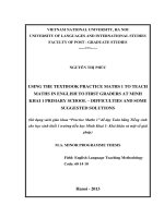
Consider the following diagram:

P(r, θ)

✟
✟

O✟

✯
✟
✟
r ✟✟✟
✟✟

✟✟
θ

✲x

The position of P is determined by its distance r from the pole and the angle, θ which the
line OP makes with the initial line, measuring this angle positively in a counter-clockwise
sense or negatively in a clockwise sense from the initial line. The notation (r, θ) denotes the
“polar co-ordinates” of the point.
5.1.2 THE RELATIONSHIP BETWEEN POLAR AND CARTESIAN CO-ORDINATES
It is convenient to superimpose the diagram for Polar Co-ordinates onto the diagram for
Cartesian Co-ordinates as follows:
y
✻


P(r, θ)
✯
✟
✟✟

r ✟✟
✟

✟
✟✟

✟✟
θ

✲x

O✟

The trigonometry of the combined diagram shows that
(a) x = r. cos θ and y = r. sin θ;
(b) r2 = x2 + y 2 and θ = tan−1 xy .
EXAMPLES

1. Express the equation
2x + 3y = 1
in polar co-ordinates.
Solution
Substituting for x and y separately, we obtain
2r cos θ + 3r sin θ = 1
That is

r=

1
2 cos θ + 3 sin θ
2


2. Express the equation
r = sin θ
in cartesian co-ordinates.
Solution
We could try substituting for r and θ separately, but it is easier, in this case, to rewrite
the equation as
r2 = r sin θ
which gives
x2 + y 2 = y
5.1.3 THE DISTANCE BETWEEN TWO POINTS
Given two points (x1 , y1 ) and (x2 , y2 ), the quantity | x2 − x1 | is called the “horizontal separation” of the two points and the quantity | y2 − y1 | is called the “vertical separation”
of the two points, assuming, of course, that the x-axis is horizontal.
The expressions for the horizontal and vertical separations remain valid even when one or
more of the co-ordinates is negative. For example, the horizontal separation of the points
(5, 7) and (−3, 2) is given by | −3 − 5 |= 8 which agrees with the fact that the two points
are on opposite sides of the y-axis.
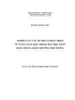
The actual distance between (x1 , y1 ) and (x2 , y2 ) is easily calculated from Pythagoras’ Theorem, using the horizontal and vertical separations of the points.

Q(x2 , y2 )

y

✟

✟
✟
✟
✟
✟✟
✟✟
✻

✟
✟
✟
O
✟
✟✟

✲x

R

✟
✟

P(x1 , y1 )

In the diagram,
PQ2 = PR2 + RQ2 .
That is,
d2 = (x2 − x1 )2 + (y2 − y1 )2 ,
giving
d=


(x2 − x1 )2 + (y2 − y1 )2 .

Note:
We do not need to include the modulus signs of the horizontal and vertical separations

3


because we are squaring them and therefore, any negative signs will disappear. For the same
reason, it does not matter which way round the points are labelled.
EXAMPLE
Calculate the distance, d, between the two points (5, −3) and (−11, −7).
Solution
Using the formula, we obtain
d=
That is,
d=

√

(5 + 11)2 + (−3 + 7)2 .
256 + 16 =

√

272 ∼
= 16.5

5.1.4 GRADIENT

The gradient of the straight-line segment, PQ, joining two points P and Q in a plane is
defined to be the tangent of the angle which PQ makes with the positive x-direction.
In practice, when the co-ordinates of the two points are P(x1 , y1 ) and Q(x2 , y2 ), the gradient,
m, is given by either
y2 − y1
m=
x2 − x1
or
y1 − y2
m=
,
x1 − x2
both giving the same result.
This is not quite the same as the ratio of the horizontal and vertical separations since we
distinguish between positive gradient and negative gradient.
EXAMPLE
Determine the gradient of the straight-line segment joining the two points (8, −13) and
(−2, 5) and hence calculate the angle which the segment makes with the positive x-direction.
Solution
m=

5 + 13
−13 − 5
=
= −1.8
−2 − 8
8+2

Hence, the angle, θ, which the segment makes with the positive x-direction is given by
tan θ = −1.8

Thus,
θ = tan−1 (−1.8)

119◦ .

5.1.5 EXERCISES
1. A square, side d, has vertices O,A,B,C (labelled counter-clockwise) where O is the pole
of a system of polar co-ordinates. Determine the polar co-ordinates of A,B and C when
4


(a) OA is the initial line;
(b) OB is the initial line.
2. Express the following cartesian equations in polar co-ordinates:
(a)
x2 + y 2 − 2y = 0;
(b)
y 2 = 4a(a − x).
3. Express the following polar equations in cartesian co-ordinates:
(a)
r2 sin 2θ = 3;
(b)
r = 1 + cos θ.
4. Determine the length of the line segment joining the following pairs of points given in
cartesian co-ordinates:
(a) (0, 0) and (3, 4);
(b) (−2, −3) and (1, 1);
(c) (−4, −6) and (−1, −2);
(d) (2, 4) and (−3, 16);
(e) (−1, 3) and (11, −2).

5. Determine the gradient of the straight-line segment joining the two points (−5, −0.5)
and (4.5, −1).
5.1.6 ANSWERS TO EXERCISES
√
1. (a) A(d, 0), B d 2, π4 , C d, π2 ;
√
(b) A d, − π4 , B(d 2, 0), C d, π4 .
2. (a) r = 2 sin θ;
(b) r2 sin2 θ = 4a(a − r cos θ).
3. (a) xy = 32 ;
(b) x4 + y 4 + 2x2 y 2 − 2x3 − 2xy 2 − y 2 = 0.
4. (a) 5; (b) 5; (c) 5; (d) 13; (e) 13.
1
5. m = − 19
.

5


“JUST THE MATHS”
UNIT NUMBER
5.2
GEOMETRY 2
(The straight line)
by
A.J.Hobson
5.2.1
5.2.2
5.2.3
5.2.4

5.2.5
5.2.6

Preamble
Standard equations of a straight line
Perpendicular straight lines
Change of origin
Exercises
Answers to exercises


UNIT 5.2 - GEOMETRY 2
THE STRAIGHT LINE
5.2.1 PREAMBLE
It is not possible to give a satisfactory diagramatic definition of a straight line since the
attempt is likely to assume a knowledge of linear measurement which, itself, depends on
the concept of a straight line. For example, it is no use defining a straight line as “the
shortest path between two points” since the word “shortest” assumes a knowledge of linear
measurement.
In fact, the straight line is defined algebraically as follows:
DEFINITION
A straight line is a set of points, (x, y), satisfying an equation of the form
ax + by + c = 0
where a, b and c are constants. This equation is called a “linear equation” and the symbol
(x, y) itself, rather than a dot on the page, represents an arbitrary point of the line.
5.2.2 STANDARD EQUATIONS OF A STRAIGHT LINE
(a) Having a given gradient and passing through the origin

y
✟✟

✟
✟

✻
✟
✟✟

✟
O
✟✟

✟
✟
✟
✟

✟✟
✟✟

✲x

✟
✟✟
✟✟

Let the gradient be m; then, from the diagram, all points (x, y) on the straight line (but no
others) satisfy the relationship,
y
= m.
x

That is,
y = mx
which is the equation of this straight line.

1


EXAMPLE
Determine, in degrees, the angle, θ, which the straight line,
√
3y = x,
makes with the positive x-direction.
Solution
The gradient of the straight line is given by
1
tan θ = √ .
3
Hence,
1
θ = tan−1 √ = 30◦ .
3
(b) Having a given gradient, and a given intercept on the vertical axis

y

✟
✟✟
✟✟

✟

✟
✟
✟✟

✻
✟
✟✟

✟
✟✟

✟
✟✟

✟
✟✟

c

✲x

O

✟

Let the gradient be m and let the intercept be c; then, in this case we can imagine that the
relationship between x and y in the previous section is altered only by adding the number c
to all of the y co-ordinates. Hence the equation of the straight line is
y = mx + c.
EXAMPLE

Determine the gradient, m, and intercept c on the y-axis of the straight line whose equation
is
7x − 5y − 3 = 0.
Solution
On rearranging the equation, we have
7
3
y = x− .
5
5
Hence,
m=
2

7
5


and

3
c=− .
5

This straight line will intersect the y-axis below the origin because the intercept is negative.
(c) Having a given gradient and passing through a given point
Let the gradient be m and let the given point be (x1 , y1 ). Then,
y = mx + c,
where
y1 = mx1 + c.

Hence, on subtracting the second of these from the first, we obtain
y − y1 = m(x − x1 ).
EXAMPLE
Determine the equation of the straight line having gradient
(−7, 2).

3
8

and passing through the point

Solution
From the formula,
3
y − 2 = (x + 7).
8
That is
8y − 16 = 3x + 21,
giving
8y = 3x + 37.
(d) Passing through two given points
Let the two given points be (x1 , y1 ) and (x2 , y2 ). Then, the gradient is given by
m=

y2 − y1
.
x2 − x1

Hence, from the previous section, the equation of the straight line is
y2 − y1

y − y1 =
(x − x1 );
x2 − x1
but this is more usually written
y − y1
x − x1
=
.
y2 − y1
x2 − x1
Note:
The same result is obtained no matter which way round the given points are taken as (x1 , y1 )
and (x2 , y2 ).
3


EXAMPLE
Determine the equation of the straight line joining the two points (−5, 3) and (2, −7), stating
the values of its gradient and its intercept on the y-axis.
Solution (Method 1).
y−3
x+5
=
,
−7 − 3
2+5
giving
7(y − 3) = −10(x + 5).
That is,
10x + 7y + 29 = 0.

Solution (Method 2).
y+7
x−2
=
,
3+7
−5 − 2
giving
−7(y + 7) = 10(x − 2).
That is,
10x + 7y + 29 = 0,
as before.
By rewriting the equation of the line as
y=−

10
29
x−
7
7

and the intercept on the y-axis is − 29
.
we see that the gradient is − 10
7
7
(e) The parametric equations of a straight line
In the previous section, the common value of the two fractions
y − y1
y2 − y1


and

x − x1
x2 − x1

is called the “parameter” of the point (x, y) and is usually denoted by t.
By equating each fraction separately to t, we obtain
x = x1 + (x2 − x1 )t

and

y = y1 + (y2 − y1 )t.

These are called the “parametric equations” of the straight line while (x1 , y1 ) and (x2 , y2 )
are known as the “base points” of the parametric representation of the line.
Notes:
(i) In the above parametric representation, (x1 , y1 ) has parameter t = 0 and (x2 , y2 ) has
parameter t = 1.
(ii) Other parametric representations of the same line can be found by using the given base
points in the opposite order, or by using a different pair of points on the line as base points.
4


EXAMPLES

1. Use parametric equations to find two other points on the line joining (3, −6) and (−1, 4).
Solution
One possible parametric representation of the line is
x = 3 − 4t


y = −6 + 10t.

To find another two points, we simply substitute any two values of t other than 0 or 1.
For example, with t = 2 and t = 3,
x = −5, y = 14

and

x = −9, y = 24.

A pair of suitable points is therefore (−5, 14) and (−9, 24).
2. The co-ordinates, x and y, of a moving particle are given, at time t, by the equations
x = 3 − 4t

and

y = 5 + 2t

Determine the gradient of the straight line along which the particle moves.
Solution
Eliminating t, we have

x−3
y−5
=
.
−4
2


That is,
2(x − 3) = −4(y − 5),
giving
2
26
y =− x+ .
4
4
Hence, the gradient of the line is
2
1
− =− .
4
2
5.2.3 PERPENDICULAR STRAIGHT LINES
The perpendicularity of two straight lines is not dependent on either their length or their
precise position in the plane. Hence, without loss of generality, we may consider two straight
line segments of equal length passing through the origin. The following diagram indicates
appropriate co-ordinates and angles to demonstrate perpendicularity:

5


Q(−b, a)

y
✻

❆
❆

❆
❆
❆

In the diagram, the gradient of OP =

P(a, b)
✟
✟✟

✟
❆O✟✟

b
a

✲x

and the gradient of OQ =

a
.
−b

Hence the product of the gradients is equal to −1 or, in other words, each gradient
is minus the reciprocal of the other gradient.
EXAMPLE
Determine the equation of the straight line which passes through the point (−2, 6) and is
perpendicular to the straight line,
3x + 5y + 11 = 0.

Solution
The gradient of the given line is − 53 which implies that the gradient of a perpendicular line
is 53 . Hence, the required line has equation
5
y − 6 = (x + 2),
3
giving
3y − 18 = 5x + 10.
That is,
3y = 5x + 28.
5.2.4 CHANGE OF ORIGIN
Given a cartesian system of reference with axes Ox and Oy, it may sometimes be convenient
to consider a new set of axes O X parallel to Ox and O Y parallel to Oy with new origin at
O whose co-ordinates are (h, k) referred to the original set of axes.

6


Y
✻

y
✻

O

✲X
✲x

O


In the above diagram, everything is drawn in the first quadrant, but the relationships obtained between the old and new co-ordinates will apply in all situations. They are
X =x−h

and

Y =y−k

x=X +h

and

y = Y + k.

or

EXAMPLE
Given the straight line,
y = 3x + 11,
determine its equation referred to new axes with new origin at the point (−2, 5).
Solution
Using
x=X −2

and

y = Y + 5,

we obtain
Y + 5 = 3(X − 2) + 11.

That is,
Y = 3X,
which is a straight line through the new origin with gradient 3.
Note:
If we had spotted that the point (−2, 5) was on the original line, the new line would be
bound to pass through the new origin; and its gradient would not alter in the change of
origin.

7


5.2.5 EXERCISES
1. Determine the equations of the following straight lines:
(a) having gradient 4 and intercept −7 on the y-axis;
(b) having gradient

1
3

and passing through the point (−2, 5);

(c) passing through the two points (1, 6) and (5, 9).
2. Determine the equation of the straight line passing through the point (1, −5) which is
perpendicular to the straight line whose cartesian equation is
x + 2y = 3.
3. Given the straight line
y = 4x + 2,
referred to axes Ox and Oy, determine its equation referred to new axes O X and O Y
with new origin at the point where x = 7 and y = −3 (assuming that Ox is parallel to
O X and Oy is parallel to O Y ).

4. Use the parametric equations of the straight line joining the two points (−3, 4) and
(7, −1) in order to find its point of intersection with the straight line whose cartesian
equation is
x − y + 4 = 0.
5.2.6 ANSWERS TO EXERCISES
1. (a)
y = 4x − 7;
(b)
3y = x + 17;
(c)
4y = 3x + 21.
2.
y = 2x − 7.
3.
Y = 4X + 33.
4.
x = −3 + 10t

y = 4 − 5t,

giving the point of intersection (at t = 51 ) as (−1, 3).

8


“JUST THE MATHS”
UNIT NUMBER
5.3
GEOMETRY 3
(Straight line laws)

by
A.J.Hobson
5.3.1
5.3.2
5.3.3
5.3.4
5.3.5

Introduction
Laws reducible to linear form
The use of logarithmic graph paper
Exercises
Answers to exercises


UNIT 5.3 - GEOMETRY 3
STRAIGHT LINE LAWS
5.3.1 INTRODUCTION
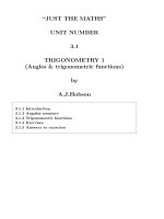
In practical work, the theory of an experiment may show that two variables, x and y, are
connected by a straight line equation (or “straight line law”) of the form
y = mx + c.
In order to estimate the values of m and c, we could use the experimental data to plot a
graph of y against x and obtain the “best straight line” passing through (or near) the
plotted points to average out any experimental errors. Points which are obviously out of
character with the rest are usually ignored.

y

x✘
✘

x ✘✘
x✘
✘x
✘
x x✘✘
✘✘✘ x

✻

✲x

O

It would seem logical, having obtained the best straight line, to measure the gradient, m,
and the intercept, c, on the y-axis. However, this not always the wisest way of proceeding
and should be avoided in general. The reasons for this are as follows:
(i) Economical use of graph paper may make it impossible to read the intercept, since this
part of the graph may be “off the page”.
(ii) The use of symbols other than x or y in scientific work may leave doubts as to which
is the equivalent of the y-axis and which is the equivalent of the x-axis. Consequently, the
gradient may be incorrectly calculated from the graph.
The safest way of finding m and c is to take two sets of readings, (x1 , y1 ) and (x2 , y2 ), from
the best straight line drawn then solve the simultaneous linear equations
1


y1 = mx1 + c,
y2 = mx2 + c.

It is a good idea if the two points chosen are as far apart as possible, since this will reduce

errors in calculation due to the use of small quantities.
5.3.2 LAWS REDUCIBLE TO LINEAR FORM
Other experimental laws which are not linear can sometimes be reduced to linear form by
using the experimental data to plot variables other than x or y, but related to them.
EXAMPLES

1. y = ax2 + b.
Method
We let X = x2 , so that y = aX + b and hence we may obtain a straight line by plotting
y against X.
2. y = ax2 + bx.
Method
Here, we need to consider the equation in the equivalent form xy = ax + b so that, by
letting Y = xy , giving Y = ax + b, a straight line will be obtained if we plot Y against
x.
Note:
If one of the sets of readings taken in the experiment happens to be
(x, y) = (0, 0), we must ignore it in this example.
3. xy = ax + b.
Method
Two alternatives are available here as follows:
(a) Letting xy = Y , giving Y = ax + b, we could plot a graph of Y against x.
(b) Writing the equation as y = a + xb , we could let
a graph of y against X.

2

1
x


= X, giving y = a + bX, and plot


4. y = axb .
Method
This kind of law brings in the properties of logarithms since, if we take logarithms of
both sides (base 10 will do here), we obtain
log10 y = log10 a + b log10 x.
Letting log10 y = Y and log10 x = X, we have
Y = log10 a + bX,
so that a straight line will be obtained by plotting Y against X.
5. y = abx .
Method
Here again, logarithms may be used to give
log10 y = log10 a + x log10 b
Letting log10 y = Y , we have
Y = log10 a + x log10 b,
which will give a straight line if we plot Y against x.
6. y = aebx .
Method
In this case, it makes sense to take natural logarithms of both sides to give
loge y = loge a + bx,
which may also be written
ln y = ln a + bx
Hence, letting ln y = Y , we can obtain a straight line by plotting a graph of Y against
x.
Note:
In all six of the above examples, it is even more important not to try to read off the gradient
and the intercept from the graph drawn. As before, we should take two sets of readings for
x (or X) and y (or Y ), substitute them in the straight-line form of the equation and solve

two simultaneous linear equations for the constants required.

3


5.3.3 THE USE OF LOGARITHMIC GRAPH PAPER
In Examples 4,5 and 6 in the previous section, it can be very tedious looking up on a
calculator the logarithms of large sets of numbers. We may use, instead, a special kind of
graph paper on which there is printed a logarithmic scale (see Unit 1.4) along one or both
of the axis directions.
0.1

0.2

0.3

0.4

1

2

3

4

10

Effectively, the logarithmic scale has already looked up the logarithms of the numbers assigned to it provided these numbers are allocated to each “cycle” of the scale in successive
powers of 10.

Data which includes numbers spread over several different successive powers of ten will need
graph paper which has at least that number of cycles in the appropriate axis direction.
For example, the numbers 0.03, 0.09, 0.17, 0.33, 1.82, 4.65, 12, 16, 20, 50 will need four
cycles on the logarithmic scale.
Accepting these restrictions, which make logarithmic graph paper less economical to use
than ordinary graph paper, all we need to do is to plot the actual values of the variables
whose logarithms we would otherwise have needed to look up. This will give the straight
line graph from which we take the usual two sets of readings; these are then substituted into
the form of the experimental equation which occurs immediately after taking logarithms of
both sides.
It will not matter which base of logarithms is being used since logarithms to two different bases are proportional to each other anyway. The logarithmic graph paper does not,
therefore, specify a base.
EXAMPLES

1. y = axb .
Method
(i) Taking logarithms (base 10), log10 y = log10 a + b log10 x.
(ii) Plot a graph of y against x, both on logarithmic scales.
(iii) Estimate the position of the “best straight line”.
(iv) Read off from the graph two sets of co-ordinates, (x1 , y1 ) and (x2 , y2 ), as far apart
as possible.

4


(v) Solve for a and b the simultaneous equations
log10 y1 = log10 a + b log10 x1 ,
log10 y2 = log10 a + b log10 x2 .

If it is possible to choose readings which are powers of 10, so much the better, but this

is not essential.
2. y = abx .
Method
(i) Taking logarithms (base 10), log10 y = log10 a + x log10 b.
(ii) Plot a graph of y against x with y on a logarithmic scale and x on a linear scale.
(iii) Estimate the position of the best straight line.
(iv) Read off from the graph two sets of co-ordinates, (x1 , y1 ) and (x2 , y2 ), as far apart
as possible.
(v) Solve for a and b the simultaneous equations
log10 y1 = log10 a + x1 log10 b,
log10 y2 = log10 a + x2 log10 b.

If it is possible to choose zero for the x1 value, so much the better, but this is not
essential.
3. y = aebx .
Method
(i) Taking natural logarithms, ln y = ln a + bx.
(ii) Plot a graph of y against x with y on a logarithmic scale and x on a linear scale.
(iii) Estimate the position of the best straight line.
(iv) Read off two sets of co-ordinates, (x1 , y1 ) and (x2 , y2 ), as far apart as possible.
(v) Solve for a and b the simultaneous equations
ln y1 = ln a + bx1 ,
ln y2 = ln a + bx2 .

If it possible to choose zero for the x1 value, so much the better, but this is not essential.
5


5.3.5 EXERCISES
In these exercises, use logarithmic graph paper where possible.

1. The following values of x and y can be represented approximately by the law y = a+bx2 :
x 0
2
4
6
8
10
y 7.76 11.8 24.4 43.6 71.2 107.0
Use a straight line graph to find approximately the values of a and b.
2. The following values of x and y are assumed to follow the law y = abx :
x 0.2
0.4
0.6
0.8
1.4
1.8
y 0.508 0.645 0.819 1.040 2.130 3.420
Use a straight line graph to find approximately the values of a and b.
3. The following values of x and y are assumed to follow the law y = aekx :
x 0.2
0.5
0.7
1.1
1.3
y 1.223 1.430 1.571 1.921 2.127
Use a straight line graph to find approximately the values of a and k.
4. The table below gives the pressure, P , and the volume, V , of a certain quantity of steam
at maximum density:
P 12.27 17.62 24.92 34.77 47.87 65.06
V 3,390 2,406 1,732 1,264 934.6 699.0

Assuming that P V n = C, use a straight line graph to find approximately the values of
n and C.
5. The coefficient of self induction, L, of a coil, and the number of turns, N , of wire are
related by the formula L = aN b , where a and b are constants.
For the following pairs of observed values, use a straight line graph to calculate approximate values of a and b:
N 25
35
50
75
150 200 250
L 1.09 2.21 5.72 9.60 44.3 76.0 156.0
6. Measurements taken, when a certain gas undergoes compression, give the following
values of pressure, p, and temperature, T :
p 10 15 20 25 35 50
T 270 289 303 315 333 353
Assuming a law of the form T = apn , use a straight line graph to calculate approximately
the values of a and n. Hence estimate the value of T when p = 32.

6


5.3.6 ANSWERS TO EXERCISES
The following answers are approximate; check only that the order of your results are correct.
Any slight variations in the position of your straight line could affect the result considerably.
1. a

8.0, b

0.99


2. a

0.4, b

3.3

3. a

1.1, k

0.5

4. n

1.06, C

5. a

1.38 × 10−3 , b

6. a

183.95, n

65887
2.08

0.17

7



“JUST THE MATHS”
UNIT NUMBER
5.4
GEOMETRY 4
(Elementary linear programming)
by
A.J.Hobson
5.4.1
5.4.2
5.4.3
5.4.4

Feasible Regions
Objective functions
Exercises
Answers to exercises


UNIT 5.4 - GEOMETRY 4
ELEMENTARY LINEAR PROGRAMMING
5.4.1 FEASIBLE REGIONS
(i) The equation, y = mx + c, of a straight line is satisfied only by points which lie on the
line. But it is useful to investigate the conditions under which a point with co-ordinates
(x, y) may lie on one side of the line or the other.
(ii) For example, the inequality y < mx + c is satisfied by points which lie below the line
and the inequality y > mx + c is satisfied by points which lie above the line.
(iii) Linear inequalities of the form Ax+By +C < 0 or Ax+By +C > 0 may be interpretted
in the same way by converting, if necessary, to one of the forms in (ii).

(iv) Weak inequalities of the form Ax + By + C ≤ 0 or Ax + By + C ≥ 0 include the points
which lie on the line itself as well as those lying on one side of it.
(v) Several simultaneous linear inequalties may be used to determine a region of the xyplane throughout which all of the inequalities are satisfied. The region is called the “feasible
region”.
EXAMPLES
1. Determine the feasible region for the simultaneous inequalities
x ≥ 0, y ≥ 0, x + y ≤ 20, and 3x + 2y ≤ 48
Solution
We require the points of the first quadrant which lie on or below the straight line
y = 20 − x and on or below the straight line y = − 23 x + 16.
The feasible region is shown as the shaded area in the following diagram:

1