Tsunami and nonlinear waves
Bạn đang xem bản rút gọn của tài liệu. Xem và tải ngay bản đầy đủ của tài liệu tại đây (10.07 MB, 319 trang )
Anjan Kundu
Tsunami and Nonlinear Waves
Anjan Kundu
(Editor)
Tsunami and
Nonlinear Waves
With 170 Figures
PROF. DR. ANJAN KUNDU
Theory Group & Centre
for Applied Mathematics
and Computational Science
Saha Institute of Nuclear Physics
Sector 1, Block AF, Bidhan Nagar
Calcutta 700064
India
e-mail:
Library of Congress Control Number: 2007921989
ISBN-13
978-3-540-71255-8 Springer Berlin Heidelberg New York
This work is subject to copyright. All rights are reserved, whether the whole or part of the
material is concerned, specifically the rights of translation, reprinting, reuse of illustrations,
recitation, broadcasting, reproduction on microfilm or in any other way, and storage in data
banks. Duplication of this publication or parts thereof is permitted only under the provisions of
the German Copyright Law of September 9, 1965, in its current version, and permission for
use must always be obtained from Springer-Verlag. Violations are liable to prosecution under
the German Copyright Law.
Springer is a part of Springer Science+Business Media
springer.com
© Springer-Verlag Berlin Heidelberg 2007
The use of general descriptive names, registered names, trademarks, etc. in this publication
does not imply, even in the absence of a specific statement, that such names are exempt
from the relevant protective laws and regulations and therefore free for general use.
Cover design: deblik, Berlin
Typesetting: camera-ready by the editor
Production: Christine Adolph
Printing: Krips bv, Meppel
Binding: Stürtz GmbH, Würzburg
Printed on acid-free paper
30/2133/ca 5 4 3 2 1 0
In memory of those died on December 26, 2004
in the Indian Ocean Tsunami
Preface
Unimaginable catastrophe struck the coasts of Indian Ocean in the morning
of January 26, 2004, wiping out more than 275,000 human life at a stroke
from the face of the earth. It was the killer Tsunami, that originated its
journey at the epicenter of the earthquake (of intensity 9.2) near Banda Aceh
in Indonesia and traveled as long as to Port Elizabeth in South Africa, covering
a distance of more than 8,000 km and bringing unprecedented devastation to
the countries like Indonesia, Thailand, Sri Lanka, India and others.
All of us were shocked saddened and felt helpless, wanted to do something in accordance to our own ability. I as a scientist working in India and
interested in nonlinear dynamics, soliton and related phenomena, decided to
contribute by organizing a dedicated effort by world experts to study different
aspects of the Tsunami and other oceanic waves with special emphasis on the
nonlinear connection of this problem. Our Centre for Appl. Math. & Comp.
Sc. (CAMCS) of our Institute, specially my colleague Prof Bikas Chakrabarti
enthusiastically supported the idea and came along with the support of a
generous fund.
In contrast to the conventional linear theory of Tsunami, our emphasis on
nonlinearity is in part related to my own conviction for its need, especially
for describing the near-shore evolution of the waves with varying depth. The
other motivation was the realization that, though a large mass of literature
is already devoted to Tsunami and related topics, no consolidated collective
study has been dedicated to nonlinear aspects of Tsunami and other oceanic
waves. This was in spite of the fact that the results obtained through conventional studies are not all convincing and conclusive and in spite of a group of
internationally well known experts, as evident from the present volume, have
long been emphasizing on the importance of nonlinearity in this regard.
Therefore as a first step we organized an international meeting on the
same topic: Tsunami & Nonlinear Waves in Saha Institute of Nuclear Physics,
Calcutta (March 6-10, 2006). That helped us not only to identify and contact the leading experts in this field, but also to spend a highly beneficial
and stimulating week in interacting and exchanging thoughts and experiences
VIII
Preface
with some of them. I am also thankful to the Springer-Verlag for offering
to publish this edited volume with interest in their Geo-Science series. This
volume is based not only on selected lectures presented in the conference
(Caputo (France), Dias (France), Fujima (Japan), Lakshmanan (India), Rao
(India), Segur (USA), Shankar (India)), but also on the contributions from
other experts well known in the field: Grimshaw (UK), Kharif (France), Madsen (Denmark), Weiss (USA), Yalciner (Turkey), Zakharov (USA) and their
collaborators, who could not participate in the conference.
This volume has 14 chapters which I have divided loosely into 2 parts:
Propagation and Source & Run up, for convenience, though many chapters
in fact are overlapping. I have also tried to arrange the chapters from more
theoretical to more application oriented, though again not in a strict sense.
The overall emphasis is on theoretical and mathematical aspects of the oceanic
waves, though the authors have given ample introduction to their subjects,
starting the material from the beginning before taking the readers to the
applicable research level with needed scientific rigor.
Hope this volume will be equally interesting and fruitful to the experts
actively working or planning to work in this field, as well as to the common
people who got interested in the subject just after 2004 and even to the
Government bureaucrats, who are forced now to take interest in such events.
Calcutta, December 2006
Anjan Kundu
Contents
Part I Propagation
Waves in shallow water, with emphasis on the tsunami of
2004
Harvey Segur . . . . . . . . . . . . . . . . . . . . . . . . . . . . . . . . . . . . . . . . . . . . . . . . . . . .
3
Integrable Nonlinear Wave Equations and Possible
Connections to Tsunami Dynamics
M. Lakshmanan . . . . . . . . . . . . . . . . . . . . . . . . . . . . . . . . . . . . . . . . . . . . . . . . . . 31
Solitary waves propagating over variable topography
Roger Grimshaw . . . . . . . . . . . . . . . . . . . . . . . . . . . . . . . . . . . . . . . . . . . . . . . . . 51
Water waves generated by a moving bottom
Denys Dutykh, Fr´ed´eric Dias . . . . . . . . . . . . . . . . . . . . . . . . . . . . . . . . . . . . . . 65
Tsunami surge in a river: a hydraulic jump in an
inhomogeneous channel
Jean-Guy Caputo, Y. A. Stepanyants . . . . . . . . . . . . . . . . . . . . . . . . . . . . . . 97
On the modelling of huge water waves called rogue waves
Christian Kharif . . . . . . . . . . . . . . . . . . . . . . . . . . . . . . . . . . . . . . . . . . . . . . . . . 113
Numerical Verification of the Hasselmann equation
Alexander O. Korotkevich, Andrei N. Pushkarev, Don Resio,
Vladimir E. Zakharov . . . . . . . . . . . . . . . . . . . . . . . . . . . . . . . . . . . . . . . . . . . . 135
Part II Source & Run up
Runup of nonlinear asymmetric waves on a plane beach
Irina Didenkulova, Efim Pelinovsky, Tarmo Soomere, Narcisse Zahibo . . 175
X
Contents
Tsunami Runup in Lagrangian Description
Koji Fujima . . . . . . . . . . . . . . . . . . . . . . . . . . . . . . . . . . . . . . . . . . . . . . . . . . . . 191
Analytical and numerical models for tsunami run-up
Per A. Madsen, David R. Fuhrman . . . . . . . . . . . . . . . . . . . . . . . . . . . . . . . . 209
Large waves caused by oceanic impacts of meteorites
Robert Weiss, Kai W¨
unnemann . . . . . . . . . . . . . . . . . . . . . . . . . . . . . . . . . . . . 237
Retracing the tsunami rays
R. Shankar . . . . . . . . . . . . . . . . . . . . . . . . . . . . . . . . . . . . . . . . . . . . . . . . . . . . . . 263
Modeling and visualization of tsunamis: Mediterranean
examples
Ahmat C. Yalciner, Effim Pelinovsky, A. Zaitsev,, A. Kurkin, C. Ozer,
H. Karakus, G. Ozyurt . . . . . . . . . . . . . . . . . . . . . . . . . . . . . . . . . . . . . . . . . . . 273
Characterization of Potential Tsunamigenic Earthquake
Source Zones in the Indian Ocean
N. Purnachandra Rao . . . . . . . . . . . . . . . . . . . . . . . . . . . . . . . . . . . . . . . . . . . . 285
Index . . . . . . . . . . . . . . . . . . . . . . . . . . . . . . . . . . . . . . . . . . . . . . . . . . . . . . . . . . 313
List of Contributors
Jean-Guy Caputo
Laboratoire de Math´ematiques,
INSA de Rouen,
B.P. 8, 76131 Mont-Saint-Aignan
cedex, France.
&
Laboratoire de Physique th´eorique
et modelisation,
Universit´e de Cergy-Pontoise and
C.N.R.S.
David R. Fuhrman
Technical University of Denmark,
Mechanical Engineering
Department, Nils Koppels All´e,
Building 403, DK-2800
Kgs. Lyngby, Denmark
Denys Dutykh
Centre de Math´ematiques
et de Leurs Applications, Ecole
Normale Sup´erieure de Cachan,
61 avenue du Pr´esident Wilson,
94235 Cachan cedex, France
Fr´
ed´
eric Dias
Centre de Math´ematiques
et de Leurs Applications, Ecole
Normale Sup´erieure de Cachan,
61 avenue du Pr´esident Wilson,
94235 Cachan cedex, France
Irina Didenkulova
Institute of Applied Physics, Nizhny
Novgorod, Russia
Koji Fujima
Dept. of Civil and Environmental
Eng., National Defense Academy.
1-10-20 Hashirimizu, Yokosuka,
239-8686 Japan.
Roger Grimshaw
Loughborough University, Loughborough, LE11 3TU, UK
H. Karakus, C. Ozer & G.
Ozyurt
Department of Civil Engineering,
Middle East Technical University,
Ocean Engineering Research Center,
06531 Ankara, Turkey
,
,
XII
List of Contributors
Christian Kharif
Institut de Recherche sur les
ph´enom`enes Hors
Equilibre, Marseille, France
Alexander O. Korotkevich
Landau Institute for Theoretical
Physics RAS 2, Kosygin Str.,
Moscow 119334, Russian Federation
A. Kurkin & A. Zaitsev
Department of Applied Mathematics,
Nizhny Novgorod State Technical
University, 24 Minin Street,
603950 Nizhny Novgorod, Russia
,
M. Lakshmanan
Centre for Nonlinear Dynamics,
School of Physics,
Bharathidasan University, Tiruchirapalli - 620 024
Per A. Madsen
Technical University of Denmark,
Mechanical Engineering
Department, Nils Koppels All´e,
Building 403, DK-2800
Kgs. Lyngby, Denmark
Waves and Solitons LLC, 918 W.
Windsong Dr., Phoenix, AZ 85045,
USA
N. Purnachandra Rao
National Geophysical Research
Institute, Hyderabad 500 007, India
Don Resio
Coastal and Hydraulics Laboratory,
U.S. Army Engineer Research and
Development Center, Halls Ferry
Rd., Vicksburg, MS 39180, USA
Harvey Segur
Department of Applied Mathematics,
University of Colorado, Boulder,
Colorado, USA
R. Shankar
The Institute of Mathematical
Sciences,
C.I.T Campus, Chennai 600113,
INDIA
Tarmo Soomere
Institute of Cybernetics, Tallinn,
Estonia
Y. A. Stepanyants
Reactor Operations, ANSTO, PMB
1, Menai (Sydney), NSW, 2234,
Australia.
Efim Pelinovsky
Institute of Applied Physics, Nizhny
Novgorod, Russia
Robert Weiss
Joint Institute for the Study of the
Atmosphere and Ocean,
University of Washington–NOAA
Andrei N. Pushkarev
Lebedev Physical Institute RAS,53,
Center for Tsunami Research,
7600 Sand Point Way NE, Seattle
Leninsky Prosp.,
WA 98115, USA
GSP-1 Moscow, 119991, Russian
Federation
List of Contributors
Kai W¨
unnemann
Institut f¨
ur Mineralogie, Museum f¨
ur
Naturkunde,
Humboldt-Universit¨
at zu Berlin,
Invalidenstrae 43,
10115 Berlin, Germany
kai.wuennemann@
museum.hu-berlin.de
Ahmet C. Yalciner,
Department of Civil Engineering,
Middle East Technical University,
Ocean Engineering Research Center,
06531 Ankara Turkey,
Narcisse Zahibo
University of Antilles and Guyane,
Guadeloupe, France
XIII
Vladimir E. Zakharov
Department of Mathematics, University of Arizona, Tucson, AZ 85721,
USA
& Lebedev Physical Institute
RAS,53, Leninsky Prosp.,
GSP-1 Moscow, 119991, Russian
Federation
& Landau Institute for Theoretical
Physics RAS 2,
Kosygin Str., Moscow 119334,
Russian Federation
& Waves and Solitons LLC, 918 W.
Windsong Dr.,
Phoenix, AZ 85045, USA
Part I
Propagation
Waves in shallow water, with emphasis on the
tsunami of 2004
Harvey Segur
Department of Applied Mathematics,
University of Colorado, Boulder, Colorado, USA
1 Introduction
This conference was organized in response to the 2004 tsunami, which killed
nearly 300,000 people in coastal communities around the Indian Ocean. We
can expect more tsunamis in the future, so now is a good time to think carefully about how to prepare for the next tsunami. With that objective, this
paper addresses three broad questions about tsunamis.
1) How do tsunamis work? Is there a simple explanation of the dynamics
of tsunamis? What makes them so much more destructive than other ocean
waves?
2) Our understanding of the theory of nonlinear waves has advanced significantly in the last forty years because of the development of “soliton theory”,
which began with the Korteweg-de Vries (KdV) equation, to be discussed below. But Korteweg & de Vries derived their now-famous equation in 1895 to
describe approximately the evolution of long waves of moderate amplitude in
shallow water of uniform depth. What does KdV theory tell us about tsunamis
in general, and about the 2004 tsunami in particular?
3) In response to the tsunami of 2004, India and other affected countries have
begun plans to implement an early warning system for tsunamis in the Indian
Ocean. On logical grounds, it seems that the requirements for such a system
should be:
•
•
•
Reliability – the system must not fail when it is needed;
Accuracy – people will lose confidence in a system that fails to predict an
important tsunami, or that predicts tsunamis that do not materialize;
Speed – an accurate tsunami-alert issued after the tsunami hits is useless.
What kind of warning system is feasible with today’s technology and meets
these requirements?
The sections that follow address each of these questions in turn. Section
2, on the basic dynamics of tsunamis, is intentionally written in nontechnical
language to make it accesible to as broad an audience as possible. The sections
4
Harvey Segur
that follow it are more technical, but the entire paper has been written to
minimize the technical expertise required by the reader.
2 Basic dynamics of tsunamis and other water waves
Water waves have broad appeal as a scientific topic, because we all have
personal experience with water waves – at the beach or in the kitchen sink. In
this paper, “water waves” refers to the waves that occur on the free surface of
a body of water, under the force of gravity. These include the waves that one
commonly sees at the beach, those in the kitchen sink, and tsunamis. Except
for very short waves (with wavelengths less than a few millimeters), waves on
the ocean’s free surface are due to the restoring force of gravity. Other kinds of
waves in the ocean, including internal waves, inertial waves and sound waves,
are not considered here.
Almost everyone has personal experience with water waves and sound
waves. But even for waves of small amplitude, these two kinds of wave systems
behave differently. Sound waves have an important property: All sound waves
travel with the same speed, independent of the frequency or wavelength of the
wave. We define “the speed of sound” to be this common speed at which all
sound waves travel. If sound waves at different frequencies traveled at different
speeds, then human communication by speech would be difficult or impossible.
Unlike sound waves, water waves with different wavelengths travel with
different speeds. For gravity-induced water waves, longer waves have lower
frequencies, and they travel faster. Figure 1 shows a series of snapshots that
illustrate this effect, but anyone can carry out a similar experiment. Drop
a rock into a quiet pond, and observe the waves patterns created. Longer
waves travel faster, so in each snapshot in Figure 1, the waves with longer
wavelengths are further away from the center of the pattern (i.e., from the
source of the disturbance), while waves with shorter wavelengths are closer to
it. As time goes on, more and more waves propagate away from the center,
but in each snapshot the longest waves in that snapshot are farthest out, and
the shortest waves are closest to the center. This property of water waves is
called “wave dispersion”.
Long water waves travel faster than short waves, but there is an upper
limit. For gravity-induced water waves of small amplitude, the maximum
speed of propagation is
c = gh
(1)
where g represents the acceleration due to gravity (about 9.8 m/sec2 at sea
level), and h is the local water depth, measured from the bottom of the water
(at the floor of the ocean, or the bottom of the water tank) up to the quiescent
free surface. All surface waves with wavelengths much longer than the local
water
speed
√ depth (and with small amplitudes) travel with an approximate
√
of gh. Thus these very long waves have a common speed, gh, which acts
Waves in shallow water, with emphasis on the tsunami of 2004
5
Fig. 1. Concentric water waves, propagating outward from a concentrated disturbance at the center. The longest waves in each snapshot are the furthest from the
disturbance, showing that long waves travel faster than short waves for gravityinduced waves on the water’s surface. These photos are a subset of the series shown
in (15) pp. 172,173, originally taken by J.W. Johnson.
like an approximate “sound speed” for the long waves (and only for them).
Because of this special property, we call a water wave a “long wave” if its
wavelength is much longer than the local water depth; equivalently, we call a
body of water “shallow water” if its depth is much less than the wavelength of
the waves in question. Both phrases
√ indicate that the relevant waves all travel
with an approximate speed of gh. This criterion is especially pertinent for
tsunamis, which have very long wavelengths.
The information in (1), plus a few measurements, is enough to provide
some understanding of the basic dynamics of the tsunami of 2004. The earthquake that generated that tsunami changed the shape of the ocean floor, by
raising the ocean floor to the west of the epicenter, and lowering it to the
east. The scale of this motion is impressive. Measured wave records indicate
that horizontal scale of the piece of seabed raised was about 100 km in the
east-west direction, and maybe 900 km in the north-south direction. The piece
of lowered seabed had similar scales. In each case, the vertical motion was a
few meters. (All of these lengths are crude estimates. The qualitative results
are unchanged if one changes any of these estimates by a factor of 2. The numbers quoted here were given by S. Ward, at />Figure 2 shows the initial shape of the 2004 tsunami, according to a computer
simulation by K. Satake, of Japan. In Figure 2, the region in red is where the
water surface was raised up by the earthquake, while the region in blue is where
it was lowered 1 (Go to http://staff.aist.go.jp/kenji.satake/animation.html
to see the entire computer simulation of the tsunami that evolved from
these initial data. A comparable simulation by S. Ward can be found at
/>1
Editor’s note: Due to conversion to b/w the color code is not visible. See the
website for colored figure.
6
Harvey Segur
Fig. 2. The shape and intensity of the initial water wave, 10 minutes after the
beginning of the earthquake. These initial conditions generated the tsunami simulated by K. Satake, at http://staff.aist.go.jp/kenji.satake/animation.html. As the
scale below the figure shows, red indicates a locally elevated water surface, while
blue indicates a depressed water surface. (Figure courtesy of K. Satake.)
We also need an estimate of the average ocean depth. According to
the average depth of
the Indian Ocean is about 3400 m. The average depth in the Bay of Bengal
is slightly less, and the earthquake that generated the 2004 tsunami occurred
near a sharp change in the ocean depth. Let us take the ocean depth west
of the epicenter of the quake (i.e., in the red region in Figure 2, or in the
Bay of Bengal) to be about 3 km, and the ocean depth east of it (in the
blue region of Figure 2, or in the Andaman Sea) to be about 1 km. (See
/>
Waves in shallow water, with emphasis on the tsunami of 2004
7
Now we can compare scales. The ratio of ocean depth to wavelength was
3
h
=
= 0.03
λ
100
1
(2)
for the waves traveling west, and even smaller for waves traveling east. So the
Indian Ocean was indeed “shallow water” for the 2004 tsunami. Moreover the
initial height of the of the wave relative to the ocean depth was
1
a
=
= 3.3 · 10−4
h
3000
1,
(3)
so the tsunami was initially very small, and (1) is applicable. According to (1),
the wave traveling west (i.e., towards India) had a speed of about 620 km/hr,
while the wave traveling east (towards Thailand) moved slower, at about 350
km/hr. (For comparison, recall that the cruising speed of a commercial jet is
about 800 km/hr.)
As we discuss in the next section, an approximate governing equation for
such a wave pattern
√ is the linear, one-dimensional wave equation, with a propagation speed of gh. A feature of that equation is that if the initial shape
of the wave is given by an east-west slice through the wave pattern shown
in Figure 2, with no initial vertical velocity (for simplicity), then this initial
shape splits into two – a wave with this spatial pattern and half the amplitude
travels east and an identical half travels west. As long as the water depth remains (approximately) constant, these waves travel with almost no change of
form. Thus, the coastal regions of India and Sri Lanka should have experienced
a positive wave (with water levels higher than normal) followed by a negative wave (with water levels lower than normal), while the coastal regions of
Thailand should have experienced the opposite: a negative wave, followed by a
positive wave. This is indeed what was reported, and this is what the computer
simulation at http://staff.aist.go.jp/kenji.satake/animation.html shows.
How would an observer experience this wave, as it traveled across the
ocean? Based on the scales quoted above, the positive wave that traveled to
the west (say) is 100 km long, and 1 m. high. That’s a lot of water, and the
wave is traveling at 620 km/hr. (A delicate point: What travels at 620 km/hr
is the rise in water height. The horizontal velocity of the water in the wave is
much smaller.) If you were sitting in a boat in the middle of the Indian Ocean,
what would you experience? The wave is moving towards you at 620 km/hr,
but it’s 100 km long, so it takes almost 10 minutes to move past your boat.
In the course of 10 minutes, therefore, your boat would move up by about
1 m, and then back down by 1 m. Unless you were extremely sensitive, you
probably would not even notice that a wave had gone by. So because of their
very long wavelengths, tsunamis are barely noticeable in the open ocean.
As the wave
√ approaches shore, everything changes. The speed of propagation is still gh , but near shore the water depth (h) decreases, and the wave
must slow down. More precisely, the front of the wave must slow down. The
back of the wave is still 100 km out at sea, so it does not slow down. The
8
Harvey Segur
consequence is that the back of the wave starts to catch up with the front,
and the wave compresses (horizontally) as it moves into shallower water. But
water is nearly incompressible, so if the wave compresses horizontally, then it
must grow vertically to accommodate the extra water that is piling up. And
the volume of water involved is enormous: about 105 m3 of water per meter
of shoreline. The deadly result is that a wave that was barely noticeable in
the open ocean can become very large and destructive near shore.
Summary: A tsunami is a very long ocean wave, usually generated by a
submarine earthquake or landslide. The wave propagates across the ocean
with a speed given approximately by (1). From these two facts, it follows that
the tsunami is barely noticeable in the open ocean, and the same tsunami can
become large and destructive near shore.
3 Theoretical models of long waves in shallow water
The mathematical theory of water waves goes back at least to Stokes
(16), who first wrote down the equations for the motion of an incompressible,
inviscid fluid, subject to a constant gravitational force, where the fluid was
bounded below by a rigid bottom and above by a free surface. (See Figure 3.)
If the motion is irrotational, then the fluid velocity can be written in terms
of a velocity potential,
u = ∇φ ,
and the velocity potential satisfies
∇2 φ = 0
for − h(x, y) < z < ζ(x, y, t)
∇φ · ∇(z + h(x, y)) = 0
on z = −h(x, y)
∂t ζ + ∂x ζ · ∂x φ + ∂y ζ · ∂y φ = ∂z φ
on z = ζ(x, y, t)
∂t φ + 12 |∇φ|2 + gζ = 0
on z = ζ(x, y, t)
,
,
,
.
(4)
The first equation, the Laplace equation, applies where there is water (i.e.,
between the fixed bottom boundary and the moving free surface). This equation says that the motion is irrotational and that water is incompressible. The
second equation says that no water can flow through the bottom boundary.
The third and fourth equations both apply on the free surface, at z = ζ(x, y, t).
The third equation says that the surface at z = ζ(x, y, t) is a free surface, while
while fourth equation says that the fluid pressure vanishes there.
These equations have been known for more than 150 years, and they are
still too hard to solve in any general sense. The difficulty is not due to the
Laplace equation, which can be solved by a variety of methods. The complication arises because an essential part of the problem is to locate the boundary
of the domain, at z = ζ(x, y, t). Until we know where the boundary is, we
cannot solve Laplace equation easily. But the boundary moves with time,
and its (changing) location is determined by solving two coupled, nonlinear,
partial differential equations. So we need the solution of Laplace equation in
Waves in shallow water, with emphasis on the tsunami of 2004
9
Fig. 3. The equations of water waves apply where there is water, shown in gray.
No water passes through the solid lower boundary at z = −h(x, y). The (moving)
upper surface is at z = ζ(x, y, t). Here x, y are horizontal coordinates, z is vertical,
∇ = (∂x , ∂y , ∂z ), and gravity g acts downward. Other possible effects (surface tension, viscosity, wind, fish, etc.) are ignored in this formulation.
order to provide the information needed for these coupled equations, and we
need information from these two coupled equations in order to solve Laplace
equation. That is the basic difficulty.
Because of this intrinsic difficulty, most advances in the theory of water
waves have come through approximations. In this approach, we abandon hope
for solving the equations in (4) in any general sense, and concentrate instead
on solving the equations approximately in some limiting situation, where the
motion simplifies. The limit relevant to tsunamis is that of long waves of small
or moderate amplitude, propagating in nearly one direction in wave of uniform
(and shallow) depth. In 1895, D. J. Korteweg & G. de Vries derived what we
now call the Kortewg-deVries (or KdV) equation,
∂τ f + f ∂ξ f + ∂ξ3 f = 0 ,
(5)
to describe wave motion in this limit. This limit has attracted a lot of attention, so there are several nearby equations, all of which are aimed at approximately the same limiting situation: (i) long waves, (ii) of small or moderate
amplitude, (iii) traveling in one direction or nearly so, (iv) in water of uniform, shallow depth, and (v) neglecting dissipation. Alternatives to (5) that
have been studied extensively in recent years are the equation of Kadomtsev
& Petviashvili ( KP, 1970),
∂ξ {∂τ f + f ∂ξ f + ∂ξ3 f } + ∂η2 f = 0 ,
(6)
an equation due to Boussinesq (1871),
∂τ2 f = c2 {∂ξ2 f + ∂ξ2 (f 2 ) + ∂ξ4 f } ,
(7)
and the equation of Camassa & Holm (1993),
∂τ m + c∂ξ f + f ∂ξ m + 2m∂ξ f + γ∂ξ3 f = 0 ,
(8)
10
Harvey Segur
where
m = f − α2 ∂ξ2 f ,
and {c, α, γ} are constants. These four equations share two unrelated properties: (i) each can be derived as an approximate model of the evolution of long
waves of moderate amplitude, propagating in nearly one direction in shallow
water of uniform depth; and (ii) each has a rich mathematical structure, called
complete integrability, which guarantees a long list of other properties including exact N-soliton solutions. (For details see (1), or any decent reference on
soliton theory.)
Fig. 4. Relevant length scales, needed to derive either the KdV or KP equation:
h is the time-averaged water height, a is a typical wave amplitude, and λ is a typical
wavelength in the direction of propagation of the waves. The KdV equation allows for
no variation normal to the direction of propagation of the waves. The KP equation
requires that the scale of variations in this normal direction (i.e., coming out of the
page in this figure) be much longer than λ.
The limit in which any of these equations apply can be stated in terms of
length scales, which must be arranged in a certain order. Three of the four
relevant lengths are shown in Figure 4. The derivation of either the KdV or
KP equation from (4) is based on four assumptions:
• Long waves (or shallow water)
h
• Small amplitude
a
• The waves move primarily in one direction
If this is exactly true, it leads to the KdV equation, (4)
If it is approximately true, it can lead to the KP equation, (5)
• All these small effects are comparable in size. For KdV, this means
ε=
a
=O
h
h
λ
λ
h
2
(9)
One imposes these assumptions self-consistently on both the velocity potential, φ(x, y, z, t), and the location of the free surface, ζ(x, y, t), in (4). (See
§4.1 of (1), for details.) At leading order (ε = 0 in a formal expansion), the
waves in question are infinitely long, infinitesimally small, and the motion at
the free surface is exactly one-dimensional. The result (if we also take h =
constant) is the one-dimensional wave equation :
∂t2 ζ = c2 ∂x2 ζ, with c2 = gh .
(10)
Waves in shallow water, with emphasis on the tsunami of 2004
11
The general solution of (10) is known. Inserting it back into the expansion for
ζ(x, y, t; ε) yields
ζ(x, y, t; ε) = εh[F (x − ct; y, εt) + G(x + ct; y, εt)] + O(ε2 ) ,
(11)
where F and G are arbitrary functions, determined from given initial data. In
words, (11) says that a signal (F ) propagates
√ to the right, and another signal
(G) propagates to the left, both with speed gh, as predicted by (1). Neither
signal changes shape as it propagates, at this order.
This partial result already provides useful information about the tsunami
of 2004. Let x represent east-west distance from the epicenter of the earthquake, with x increasing to the east. Then F represents the wave that propagated towards Thailand, while G represents the wave that propagated towards India. The initial shape of F and G were determined by the initial data
from the earthquake, shown approximately in Figure 2. The G-wave, which
propagated towards India, traveled approximately 1500 km cross the Bay of
Bengal in slightly over 2 hours. The west-going G-wave wave had a positive
region (i.e., extra water) in front, with a negative region (a deficit of water) behind. As it propagated across the Bay of Bengal, this shape remained
approximately constant according to (11), and as shown in the animation at
http://staff.aist.go.jp/kenji.satake/animation.html. As discussed in Section 2,
the wave changed its shape entirely when it entered the shallow coastal regions
where h changes, and where the assumptions in (9) break down. Even so, the
wave that entered India’s coastal region had a positive wave (i.e., with extra
water) in front, with a negative wave (with a deficit of water) behind. This is
what inundated regions of India experienced. The F -wave, which propagated
towards Thailand, was moving slower, but the distance across the Andaman
Sea was also smaller. It took 1-2 hours to reach land in Thailand. As it traveled, it had a negative wave in front, followed by a positive wave behind. This
is consistent with what inundated regions of Thailand experienced.
Now return to the derivation of (5), the KdV equation, from (4). We may
follow (for example) the F -wave √
by changing to a coordinate system that
moves with the F -wave, at speed gh. Set
√
ε
(x − t gh) .
(12)
ξ=
h
At leading order, according to (10), F does not change in this coordinate
system, so we may proceed to the next order, O(ε2 ). Now the small effects
that were ignored at leading order (i.e., that the wave amplitude is small but
not infinitesimal, that the wave length is long but not infinitely long, and that
slow transverse variations are allowed) can be observed. Each effect is small,
but over a long distance these small effects can build up, to have a significant
cumulative effect on F . To capture this slow evolution of F , we introduce a
slow time-scale,
εg
τ = εt
,
(13)
h
12
Harvey Segur
and find that F satisfies approximately the KdV equation,
1
2∂τ F + 3F ∂ξ F + ∂ξ3 F = 0 ,
3
(14)
if the surface waves are strictly one-dimensional, or the KP equation,
1
∂ξ (2∂τ F + 3F ∂ξ F + ∂ξ3 F ) + ∂η2 F = 0
3
(15)
if the surface patterns are weakly two-dimensional. After rescaling the variables in (14) or (15) to absorb constants, (14) becomes (5), and (15) becomes
(6).
In words, (10) & (11) say that on a short time-scale, the right-going wave
does not change (so ∂τ F = 0) in the coordinate system given by (12,13). On
a longer time-scale, the KdV equation (14) describes how F changes slowly,
due to weak nonlinearity (F ∂ξ F ) and weak dispersion (∂ξ3 F ). Alternatively,
the KP equation (15) allows F to change because of these two weak effects
and also because of weak two-dimensionality (∂η2 F ).
The KdV and KP equations have been derived in many physical contexts, and they always have the same physical meaning: on a short time-scale,
the leading-order equation is the one-dimensional, linear wave equation; on a
longer time scale, each of the two free waves that make up the solution of the
1-D wave equation satisfies its own KdV (or KP) equation, so each of the two
waves changes slowly because of the cumulative effect of weak nonlinearity,
weak dispersion and (for KP) weak two-dimensionality.
How does this theory apply to the tsunami of 2004? For the wave that
propagated towards India and Sri Lanka, the two parameters required to be
small are (from (2))
1
a
=
= 3 · 10−4 ,
h
3000
h
λ
2
=
3
100
2
= 9 · 10−4 .
Both numbers are much smaller than 1, and they are comparable to each
other. In addition, the length scale of the affected seabed in the north-south
direction (900 km) was significantly longer than the wavelength in the eastwest direction (100 km), so the initial wave propagation was approximately
one-dimensional. At leading order, therefore, the 2004 tsunami is a good candidate for KdV theory.
But a problem arises at the next order. The KdV equation describes approximately the dynamics of the propagating wave on a slow time-scale. One
can see from (12,13) that the time required to see KdV dynamics is longer by
a factor of about 1ε than a typical time scale for (10). Equivalently, the propagation distance required to see KdV dynamics is approximately 1ε longer
than a typical length scale of the problem. The scaling above uses the water
depth, h, as the fundamental length-scale, so the distance required for the
westward propagating wave (which struck India and Sri Lanka) to show KdV
dynamics was about
Waves in shallow water, with emphasis on the tsunami of 2004
D∼
13
h
= 3 · 3000 ∼ 104 km .
ε
But the distance across the Bay of Bengal is nowhere much more than 1500
km, much too short for KdV dynamics to develop. For the eastward propagating wave (which struck Thailand) the wave speed is slower, but the maximal distances are also smaller, and the conclusion is the same. For the 2004
tsunami, the propagation distances from the epicenter of the earthquake to
India, Sri Lanka, or Thailand were much too short for KdV dynamics to develop.
This conclusion applies to the 2004 tsunami, and probably to any future
tsunami generated in same geological fault region (near Sumatra, and where
the tectonic plate that contains India is subducting beneath the plate that contains Burma). Even so, during this conference Prof. M. Lakshmanan observed
correctly that the conclusion does not apply to all tsunamis. He pointed out
that the 1960 Chilean earthquake, the largest earthquake ever recorded (magnitude 9.6 on a Richter scale), produced a tsunami that propagated across
the Pacific Ocean. It reached Hawaii after 15 hours, Japan after 22 hours,
and it caused massive destruction in both places. This tsunami propagated
over a long enough distance that KdV dynamics were probably relevant. For
more information about this earthquake and its tsunami, see (13), (14), or
depot/world/1960 05 22 tsunami.html.
Why does it matter whether KdV dynamics apply to tsunamis? One appealing feature of integrable equations, like those in (5)-(8), is that they are
nonlinear partial differential equations that can be solved exactly, as initialvalue problems. (See (1), for details.) For the KdV equation, (14), starting with
arbitrary initial data that are smooth and sufficiently localized in space, the
solution that evolves from these data evolves into a finite number of discrete,
localized, positive waves (called solitons), plus an oscillatory tail. Each soliton
retains its localized identity forever, while the oscillatory tail
√ disperses and
spreads out in space. All solitons travel slightly faster than gh, and taller
solitons travel
√ faster than shorter ones. The oscillatory tail travels slightly
slower than gh, so after a long time the solution evolves into an ordered set
of solitons, with the tallest in front, followed by an oscillatory tail. The details
of this general picture can be predicted fairly easily from detailed knowledge
of the initial data.
In the early 1970s, Joe Hammack carried out a series of laboratory experiments on the dynamics of long waves in shallow water, and Hammack
& Segur (1974,1978a,b) used his data to test the predictions of KdV theory.
The motivation for their work was closely related to the motivation for this
conference: Can KdV theory be used effectively to predict tsunamis? One of
their conclusions was that KdV dynamics do not occur unless the propagation
distance is long enough, as discussed above. A second major conclusion was
the importance of the wave volume in the initial data, which we discuss next.
14
Harvey Segur
Fig. 5. Schematic diagram of wave maker, used by J.L. Hammack to create waves
in shallow water. See (6) or (7) for more details.
Hammack’s experiments were carried out in a long wave tank. At one end
of the tank was a piston that spanned the width of the tank, as shown in
Figure 5 and as discussed in detail in (6). The piston was programmed to
move up or down in a controlled way, and its vertical motion was intended to
approximate the motion of the ocean floor during a submarine earthquake. If
the piston moved up (or down) quickly enough, then the water surface above
the piston moved up (or down) with it, after which this positive (or negative)
surface wave propagated from one end of the tank to the other. Measuring
probes, positioned at either four or five separate locations along the tank,
measured the shape of the wave as it propagated the length of the tank.
The results of one set of experiments are shown in Figure 6. Each column in
this figure provides information about one of the three experiments in this set.
The top picture in each column shows the time-history of the paddle motion
for that experiment – in the first experiment the paddle was raised smoothly
from one elevation to another. The piston motion was fast enough that the
water above it simply rose along with it, so the shape of the wave observed at
the first measuring station (at x/h = 0 in the first column) is closely related
to the shape of the paddle – approximately a rectangular box. Moving down
the first column, the next picture shows the
√ wave observed at x/h = 20, in
a coordinate system moving with speed gh. Equation (10)
√ predicts that
the wave does not change, provided we travel with speed gh, and little
or no change is observed over this short distance. Over long distances, KdV
theory predicts that this initially positive wave should evolve into four solitons,
ordered in size, and four solitons are observed at x/h = 400. [Within each wave
record the wave is propagating to the left, so at x/h = 180 or at x/h = 400
the tallest soliton is out in front, as KdV theory predicts.] In this experiment,
the oscillatory tail is very small and barely visible.
Anyone who has experienced a serious earthquake knows that the monotonically rising piston motion shown in the first column is too simple to describe ground motion during an actual earthquake. So the experiments in the
second and third columns had the same mean piston motion as that in the