12
Pattern Classi cation and Diagnostic
Decision

The nal purpose of biomedical image analysis is to classify a given image, or
the features that have been detected in the image, into one of a few known
categories. In medical applications, a further goal is to arrive at a diagnostic decision regarding the condition of the patient. A physician or medical
specialist may achieve this goal via visual analysis of the image and data
presented: comparative analysis of the given image with others of known diagnoses or the application of established protocols and sets of rules assist in
such a decision-making process. Images taken earlier of the same patient may
also be used, when available, for comparative or di erential analysis. Some
measurements may also be made from the given image to assist in the analysis. The basic knowledge, clinical experience, expertise, and intuition of the
physician play signi cant roles in this process.
When image analysis is performed via the application of computer algorithms, the typical result is the extraction of a number of numerical features.
When the numerical features relate directly to measurements of organs or
features represented by the image | such as an estimate of the size of the
heart or the volume of a tumor | the clinical specialist may be able to use
the features directly in his or her diagnostic logic. However, when parameters such as measures of texture and shape complexity are derived, a human
analyst is not likely to be able to analyze or comprehend the features. Furthermore, as the number of the computed features increases, the associated
diagnostic logic may become too complicated and unwieldy for human analysis. Computer methods would then be desirable to perform the classi cation
and decision process.
At the outset, it should be borne in mind that a biomedical image forms but
one piece of information in arriving at a diagnosis: the classi cation of a given
image into one of many categories may assist in the diagnostic procedure,
but will almost never be the only factor. Regardless, pattern classi cation
based upon image analysis is indeed an important aspect of biomedical image
analysis, and forms the theme of the present chapter. Remaining within the
realm of CAD as introduced in Figure 1.33 and Section 1.11, it would be
preferable to design methods so as to aid a medical specialist in arriving at a
diagnosis rather than to provide a decision.
© 2005 by CRC Press LLC

1089


1090

Biomedical Image Analysis

A generic problem statement for pattern classi cation may be expressed as
follows: A number of measures and features have been derived from a biomedical image. Develop methods to classify the image into one of a few specied categories. Investigate the relevance of the features and the classi cation
methods in arriving at a diagnostic decision about the patient.
Observe that the features mentioned above may have been derived manually
or by computer methods. Recognize the distinction between classifying the
given image and arriving at a diagnosis regarding the patient: the connection
between the two tasks or steps may not always be direct. In other words, a
pattern classi cation method may facilitate the labeling of a given image as
being a member of a particular class arriving at a diagnosis of the condition of
the patient will most likely require the analysis of several other items of clinical
information. Although it is common to work with a prespeci ed number of
pattern classes, many problems do exist where the number of classes is not
known a priori. A special case is screening, where the aim is to simply decide
on the presence or absence of a certain type of abnormality or disease. The
initial decision in screening may be further focused on whether the subject
appears to be free of the speci c abnormality of concern or requires further
investigation.
The problem statement and description above are rather generic. Several
considerations arise in the practical application of the concepts mentioned
above to medical images and diagnosis. Using the detection of breast cancer as an example, the following questions illustrate some of the problems
encountered in practice.
Is a mass or tumor present? (Yes/No)

If a mass or tumor is present
{ Give or mark its location.
{ Compare the density of the mass to that of the surrounding tissues:
hypodense, isodense, hyperdense.
{ Describe the shape of its boundary: round, ovoid, irregular, macrolobulated, microlobulated, spiculated.
{ Describe its texture: homogeneous, heterogeneous, fatty.
{ Describe its edge: sharp (well-circumscribed), ill-de ned (fuzzy).
{ Decide if it is a benign mass, a cyst (solid or uid- lled), or a
malignant tumor.
Are calci cations present? (Yes/No)
If calci cations are present:
{ Estimate their number per cm2 .
{ Describe their shape: round, ovoid, elongated, branching, rough,
punctate, irregular, amorphous.
© 2005 by CRC Press LLC


Pattern Classi cation and Diagnostic Decision

1091

{ Describe their spatial distribution or cluster.
{ Describe their density: homogeneous, heterogeneous.
Are there signs of architectural distortion? (Yes/No)
Are there signs of bilateral asymmetry? (Yes/No)
Are there major changes compared to the previous mammogram of the
patient?
Is the case normal? (Yes/No)
If the case is abnormal:
{ Is the disease benign or malignant (cancer)?

The items listed above give a selection of the many features of mammograms that a radiologist would investigate see Ackerman et al. 1084] and the
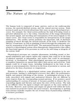
BI-RADSTM manual 403] for more details. Figure 12.1 shows a graphical user
interface developed by Alto et al. 528, 1085] for the categorization of breast
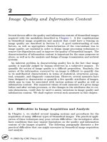
masses related to some of the questions listed above. Figure 12.2 illustrates
four segments of mammograms demonstrating masses and tumors of di erent characteristics, progressing from a well-circumscribed and homogeneous
benign mass to a highly spiculated and heterogeneous tumor.
The subject matter of this book | image analysis and pattern classi cation | can provide assistance in responding to only some of the questions
listed above. Even an entire set of mammograms may not lead to a nal
decision: other modes of diagnostic imaging and means of investigation may
be necessary to arrive at a de nite diagnosis.
In the following sections, a number of methods for pattern classi cation,
decision making, and evaluation of the results of classi cation are reviewed
and illustrated.
(Note: Parts of this chapter are reproduced, with permission, from R.M.
Rangayyan, Biomedical Signal Analysis: A Case-Study Approach, IEEE Press
and Wiley, New York, NY. 2002, c IEEE.)

12.1 Pattern Classi cation

Pattern recognition or classi cation may be de ned as the categorization of
the input data into identi able classes via the extraction of signi cant features
or attributes of the data from a background of irrelevant detail 402, 721,
1086, 1087, 1088, 1089, 1090]. In biomedical image analysis, after quantitative
features have been extracted from the given images, each image (or ROI) may
be represented by a feature vector x = x1 x2 : : : xn ]T , which is also known
© 2005 by CRC Press LLC


1092


FIGURE 12.1

Biomedical Image Analysis

Graphical user interface for the categorization of breast masses. Reproduced
with permission from H. Alto, R.M. Rangayyan, R.B. Paranjape, J.E.L.
Desautels, and H. Bryant, \An indexed atlas of digital mammograms for
computer-aided diagnosis of breast cancer", Annales des Telecommunications,
58(5): 820 { 835, 2003. c GET { Lavoisier. Figure courtesy of C. LeGuillou, Ecole Nationale Superieure des Telecommunications de Bretagne, Brest,
France.

© 2005 by CRC Press LLC


Pattern Classi cation and Diagnostic Decision

(a) b145lc95
fcc = 0.00
SI = 0.04
cf = 0.11
A = 0.07
F8 = 8.11

(b) b164ro94
0.42
0.18
0.26
0.08
8.05


FIGURE 12.2

(c) m51rc97
0.64
0.49
0.55
0.09
8.15

1093

(d) m55lo97
0.83
0.61
0.99
0.01
8.29

Examples of breast mass regions and contours with the corresponding values
of fractional concavity fcc , spiculation index SI , compactness cf , acutance
A, and sum entropy F8 . (a) Circumscribed benign mass. (b) Macrolobulated
benign mass. (c) Microlobulated malignant tumor. (d) Spiculated malignant
tumor. Note that the masses and their contours are of widely di ering size,
but have been scaled to the same size in the illustration. The rst letter
of the case identi er indicates a malignant diagnosis with `m' and a benign
diagnosis with `b' based upon biopsy. The symbols after the rst numerical
portion of the identi er represent l: left, r: right, c: cranio-caudal view, o:
medio-lateral oblique view, x: axillary view. The last two digits represent
the year of acquisition of the mammogram. An additional character of the
identi er after the year (a { f), if present, indicates the existence of multiple

masses visible in the same mammogram. Reproduced with permission from
H. Alto, R.M. Rangayyan, and J.E.L. Desautels, \Content-based retrieval and
analysis of mammographic masses", Journal of Electronic Imaging, in press,
2005. c SPIE and IS&T.

© 2005 by CRC Press LLC


1094

Biomedical Image Analysis

as the measurement vector or a pattern vector. When the values xi are real
numbers, x is a point in an n-dimensional Euclidean space: vectors of similar
objects may be expected to form clusters as illustrated in Figure 12.3.
x

x

2

x

x

x
x

class C
z

1
2 x
x
x
x
x

decision function
d( x)= w x + w x + w = 0
o oo
1 1
2 2
3
o o o
z
o 1o o
o oo
o
class C
2
x

1

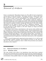
FIGURE 12.3

Two-dimensional feature vectors of two classes, C1 and C2 . The prototypes
of the two classes are indicated by the vectors z1 and z2 . The linear decision
function d(x) shown (solid line) is the perpendicular bisector of the straight
line joining the two prototypes (dashed line). Reproduced with permission

from R.M. Rangayyan, Biomedical Signal Analysis: A Case-Study Approach,
IEEE Press and Wiley, New York, NY. 2002, c IEEE.
For e cient pattern classi cation, measurements that could lead to disjoint sets or clusters of feature vectors are desired. This point underlines the
importance of the appropriate design of the preprocessing and feature extraction procedures. Features or characterizing attributes that are common to all
patterns belonging to a particular class are known as intraset or intraclass
features. Discriminant features that represent the di erences between pattern
classes are called interset or interclass features.

The pattern classi cation problem is that of generating optimal decision
boundaries or decision procedures to separate the data into pattern classes
based on the feature vectors provided. Figure 12.3 illustrates a simple linear
decision function or boundary to separate 2D feature vectors into two classes.
© 2005 by CRC Press LLC


Pattern Classi cation and Diagnostic Decision

1095

12.2 Supervised Pattern Classi cation

The problem considered in supervised pattern classi cation may be stated
as follows: You are provided with a number of feature vectors with classes
assigned to them. Propose techniques to characterize and parameterize the
boundaries that separate the classes.
A given set of feature vectors of known categorization is often referred to
as a training set. The availability of a training set facilitates the development
of mathematical functions that can characterize the separation between the
classes. The functions may then be applied to new feature vectors of unknown
classes to classify or recognize them. This approach is known as supervised

pattern classi cation. A set of feature vectors of known categorization that
is used to evaluate a classi er designed in this manner is referred to as a test
set. After adequate testing and con rmation of the method with satisfactory
results, the classi er may be applied to new feature vectors of unknown classes
the results may then be used to arrive at diagnostic decisions. The following
subsections describe a few methods that can assist in the development of
discriminant and decision functions.

12.2.1 Discriminant and decision functions

A general linear discriminant or decision function is of the form
d(x) = w1 x1 + w2 x2 + + wn xn + wn+1 = wT x
(12.1)
where x = x1 x2 : : : xn 1]T is the feature vector augmented by an additional
entry equal to unity, and w = w1 w2 : : : wn wn+1 ]T is a correspondingly
augmented weight vector. A two-class pattern classi cation problem may be
stated as
d(x) = wT x > 00 ifif xx 22 CC1
(12.2)
2
where C1 and C2 represent the two classes. The discriminant function may be
interpreted as the boundary separating the classes C1 and C2 , as illustrated
in Figure 12.3.
In the general case of an M -class pattern classi cation problem, we will
need M weight vectors and M decision functions to perform the following
decisions:
x 2 Ci i = 1 2 : : : M
di (x) = wiT x > 00 ifotherwise
(12.3)
where wi = (wi1 wi2 ::: win wi n+1 )T is the weight vector for the class Ci .

Three cases arise in solving this problem 1086]:
Case 1: Each class is separable from the rest by a single decision surface:
if di (x) > 0 then x 2 Ci :
(12.4)
© 2005 by CRC Press LLC


1096

Biomedical Image Analysis

Case 2: Each class is separable from every other individual class by a distinct

decision surface, that is, the classes are pairwise separable. There are
M (M ; 1)=2 decision surfaces given by dij (x) = wijT x.
if dij (x) > 0 8 j 6= i then x 2 Ci :

(12.5)

Note: dij (x) = ;dji (x).]
Case 3: There exist M decision functions dk (x) = wkT x k = 1 2 : : : M
with the property that

if di (x) > dj (x) 8 j 6= i then x 2 Ci :

(12.6)

This is a special instance of Case 2. We may de ne

dij (x) = di (x) ; dj (x) = (wi ; wj )T x = wijT x:


(12.7)

If the classes are separable under Case 3, they are separable under Case
2 the converse is, in general, not true.
Patterns that may be separated by linear decision functions as above are
said to be linearly separable. In other situations, an in nite variety of complex
decision boundaries may be formulated by using generalized decision functions
based upon nonlinear functions of the feature vectors as

d(x) = w1 f1 (x) + w2 f2 (x) +
=

KX
+1
i=1

wi fi (x):

+ wK fK (x) + wK +1

(12.8)
(12.9)

Here, ffi (x)g i = 1 2 : : : K are real, single-valued functions of x fK +1 (x) =
1. Whereas the functions fi (x) may be nonlinear in the n-dimensional space
of x, the decision function may be formulated as a linear function by de ning a transformed feature vector xy = f1 (x) f2 (x) : : : fK (x) 1]T . Then,
d(x) = wT xy , with w = w1 w2 : : : wK wK +1 ]T : Once evaluated, ffi (x)g is
just a set of numerical values, and xy is simply a K -dimensional vector augmented by an entry equal to unity. Several methods exist for the derivation
of optimal linear discriminant functions 402, 738, 674].

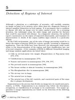
Example of application: The ROIs of 57 breast masses are shown in
Figure 12.4 arranged in the order of decreasing acutance A (see Sections 2.15,
7.9.2, and 12.12). Figure 12.5 shows the contours of the 57 masses arranged in
the increasing order of fractional concavity fcc (see Section 6.4). Most of the
contours of the benign masses are seen to be smooth, whereas most of the contours of the malignant tumors are rough and spiculated. Furthermore, most of
the benign masses have well-de ned, sharp edges and are well-circumscribed,
whereas the majority of the malignant tumors possess ill-de ned and fuzzy
borders. It is seen that the shape factor fcc facilitates the ordering of the
© 2005 by CRC Press LLC


Pattern Classi cation and Diagnostic Decision

1097

contours in terms of shape complexity. However, the contours of a few benign masses and a few malignant tumors do not follow the expected trend.
In addition, the acutance measure has lower values for most of the malignant
tumors than for a majority of the benign masses.
The three shape factors cf , fcc , and SI (see Chapter 6) the 14 texture
measures as de ned by Haralick 441, 442] (see Section 7.3) and four measures
of edge sharpness as de ned by Mudigonda et al. 165] (see Section 7.9.2) were
computed for the ROIs and their contours. (Note: The factor SI was divided
by two in this example to reduce it to the range 0 1].) Figure 12.6 gives a plot
of the 3D feature-vector space (fcc A F8 ) for the 57 masses. The feature F8
shows poor separation between the benign and malignant samples, whereas
the feature A demonstrates some degree of separation. A scatter plot of the
three shape factors (fcc cf SI ) of the 57 masses is given in Figure 12.7. Each
of the three shape factors demonstrates high discriminant capability.
Figure 12.8 shows a 2D plot of the shape-factor vectors fcc SI ] for a training set formed by selecting the vectors for 18 benign masses and 10 malignant
tumors. The prototypes for the benign and malignant classes, obtained by averaging the vectors over all the members of the two classes in the training set,

are marked as `B' and `M', respectively, on the plot. The solid straight line is
the perpendicular bisector of the line joining the two prototypes (dashed line),
and represents a linear discriminant function. The equation of the straight
line is SI + 0:6826 fcc ; 0:5251 = 0: The decision function is represented by
the following rule:
if SI + 0:6826 fcc ; 0:5251 < 0 then
benign mass
else
malignant tumor
end.
It is seen that the rule given above will correctly classify all of the training
samples.
Figure 12.9 shows the result of application of the linear discriminant function designed and shown in Figure 12.8 to a test set of 19 benign masses and
10 malignant tumors. The test set does not include any of the cases from the
training set. It is seen that the classi er will lead to three false negatives in
the test set.

12.2.2 Distance functions

Consider M pattern classes represented by their prototype patterns z1 z2
: : : zM . The prototype of a class is typically computed as the average of all
the feature vectors belonging to the class. Figure 12.3 illustrates schematically
the prototypes z1 and z2 of the two classes shown.
© 2005 by CRC Press LLC


1098

Biomedical Image Analysis


m51rc97 0.088

b164ro94 0.085

b164rc94 0.085

b146ro96 0.084

b62lc97 0.084

b62lo97 0.080

b155ro95 0.080

m23lc97 0.079

b155rc95 0.078

m23lo97 0.074

m63ro97 0.073

b62lx97 0.072

b145lc95 0.071

b166lc94 0.069

b146rc96 0.068


b62rc97e 0.065

b62rc97d 0.064

m63rc97 0.064

b62rc97a 0.063

b62rc97b 0.063

b164rx94 0.063

b62ro97e 0.063

b145lo95 0.062

b62ro97a 0.059

b110rc95 0.059

b148ro97 0.058

b157lc96 0.057

b62ro97d 0.057

b157lo96 0.056

b110ro95 0.055


b62ro97c 0.054

b62rc97c 0.053

b64rc97 0.052

b161lc95 0.051

m22lo97 0.051

m62lx97 0.051

b62rc97f 0.051

b148rc97 0.050

b166lo94 0.050

m59lc97 0.049

b158lc95 0.047

m22lc97 0.046

b62ro97b 0.045

m58rm97 0.044

b161lo95 0.043


m59lo97 0.041

m61lc97 0.040

b158lo95 0.039

b62ro97f 0.036

m51ro97 0.033

m64lc97 0.029

m62lo97 0.029

m55lc97 0.027

m61lo97 0.024

m58ro97 0.021

m58rc97 0.014

m55lo97 0.012

FIGURE 12.4

ROIs of 57 breast masses, including 37 benign masses and 20 malignant tumors. The
ROIs are arranged in the order of decreasing acutance A. Note that the masses are
of widely di ering size, but have been scaled to the same size in the illustration. For
details regarding the case identi ers, see Figure 12.2. Reproduced with permission

from H. Alto, R.M. Rangayyan, and J.E.L. Desautels, \Content-based retrieval and
analysis of mammographic masses", Journal of Electronic Imaging, in press, 2005.
c SPIE and IS&T.
© 2005 by CRC Press LLC


Pattern Classi cation and Diagnostic Decision

1099

b145lc95 0

b146rc96 0

b148rc97 0

b148ro97 0

b161lc95 0

b62rc97e 0

b62lo97 0.017

b164rx94 0.028

b62rc97a 0.03

b62rc97b 0.033


b110rc95 0.035

b62ro97e 0.041

b161lo95 0.05

b62lx97 0.052

b62rc97d 0.061

b158lo95 0.063

b164rc94 0.064

b145lo95 0.074

b62ro97b 0.091

b110ro95 0.094

b155rc95 0.098

b62ro97f 0.099

b157lo96 0.13

b62rc97c 0.15

b166lo94 0.15


b166lc94 0.17

b62ro97d 0.17

b157lc96 0.2

b62lc97 0.2

b155ro95 0.2

b62rc97f 0.2

b62ro97a 0.22

b146ro96 0.22

b62ro97c 0.24

b164ro94 0.24

b158lc95 0.26

m63ro97 0.29

m62lx97 0.29

b64rc97 0.31

m51rc97 0.37


m23lc97 0.39

m55lc97 0.41

m59lo97 0.42

m23lo97 0.42

m59lc97 0.43

m63rc97 0.44

m51ro97 0.44

m58rc97 0.45

m58ro97 0.46

m61lo97 0.47

m22lc97 0.47

m55lo97 0.48

m58rm97 0.5

m61lc97 0.5

m62lo97 0.5


m64lc97 0.5

m22lo97 0.57

FIGURE 12.5

Contours of 57 breast masses, including 37 benign masses and 20 malignant tumors.
The contours are arranged in the order of increasing fcc . Note that the masses and
their contours are of widely di ering size, but have been scaled to the same size
in the illustration. For details regarding the case identi ers, see Figure 12.2. See
also Figure 12.30. Reproduced with permission from H. Alto, R.M. Rangayyan, and
J.E.L. Desautels, \Content-based retrieval and analysis of mammographic masses",
Journal of Electronic Imaging, in press, 2005. c SPIE and IS&T.
© 2005 by CRC Press LLC


1100

Biomedical Image Analysis

1

Sum Entropy

0.8

0.6

0.4


0.2

1
0.8

0
1

0.6
0.8

0.4

0.6
0.4
Acuta

nce

FIGURE 12.6

0.2
0.2
0

0

na

tio


ac

Fr

ity

av

nc

o
lC

Plot of the 3D feature-vector space (fcc A F8 ) for the set of 57 masses in
Figure 12.4. `o': benign masses (37). ` ': malignant tumors (20). Reproduced with permission from H. Alto, R.M. Rangayyan, and J.E.L. Desautels,
\Content-based retrieval and analysis of mammographic masses", Journal of
Electronic Imaging, in press, 2005. c SPIE and IS&T.

© 2005 by CRC Press LLC


Pattern Classi cation and Diagnostic Decision

1101

0.8

0.7


Spiculation Index

0.6

0.5

0.4

0.3

0.2

0.1

0
0

0.2

0.4

0.6

0.8

0

Compactness

0.1


0.3

0.2

0.4

0.5

l Concavity

Fractiona

FIGURE 12.7

Plot of the 3D feature-vector space (fcc cf SI ) for the set of 57 contours in
Figure 12.5. `o': benign masses (37). ` ': malignant tumors (20). Figure
courtesy of H. Alto.
The Euclidean distance between an arbitrary pattern vector x and the ith
prototype is given as

q

Di = kx ; zi k = (x ; zi )T (x ; zi ):

(12.10)

A simple rule to classify the pattern vector x would be to choose that class
for which the vector has the smallest distance:
if Di < Dj 8 j 6= i then x 2 Ci :


(12.11)

(See Section 12.12 for the description of an application of the Euclidean distance to the analysis of breast masses and tumors.)
A simple relationship may be established between discriminant functions
and distance functions as follows 1086]:

Di2 = kx ; zi k2 = (x ; zi )T (x ; zi )

= xT x ; 2xT zi + zTi zi = xT x ; 2 xT zi ; 21 zTi zi :

(12.12)

Choosing the minimum of Di2 is equivalent to choosing the minimum of
Di (because all Di > 0). Furthermore, from the equation above, it follows
© 2005 by CRC Press LLC


1102

Biomedical Image Analysis

1

0.9

x

0.8


x x
x

x

Spiculation index SI

0.7
Mx

0.6
x
0.5

x
x

0.4

0.3

x

0.2
o
o
o o
0.1
o
o o B o

o o
o
o
oo
0
0
0.1

o
o o

0.2

FIGURE 12.8

0.3

0.4
0.5
0.6
Fractional concavity fcc

0.7

0.8

0.9

1


Plot of the 2D feature-vector space (fcc SI ) for the training set of 18 benign masses (`o') and 10 malignant tumors (`x') selected from the dataset in
Figure 12.5. The prototypes of the two classes are indicated by the vectors
marked `B' and `M'. The solid line shown is a linear decision function, obtained
as the perpendicular bisector of the straight line joining the two prototypes
(dashed line).

© 2005 by CRC Press LLC


Pattern Classi cation and Diagnostic Decision

1103

1

0.9
x

x
0.8

x
x

Spiculation index SI

0.7
x

0.6


x

0.5
x
0.4

0.3

0.2

o
o

0.1 o o
o
o
o oo oo
0

0

0.1

o
o
o

o o
o

o

0.2

FIGURE 12.9

x

x
x

0.3

0.4
0.5
0.6
Fractional concavity fcc

0.7

0.8

0.9

1

Plot of the 2D feature-vector space (fcc SI ) for the test set of 19 benign masses
(`o') and 10 malignant tumors (`x') selected from the dataset in Figure 12.5.
The solid line shown is a linear decision function designed as illustrated in
Figure 12.8. Three malignant cases are misclassi ed by the decision function

shown.

© 2005 by CRC Press LLC


1104

Biomedical Image Analysis

that choosing the minimum of Di2 is equivalent to choosing the maximum of
(xT zi ; 12 zTi zi ). Therefore, we may de ne the decision function
di (x) = xT zi ; 12 zTi zi i = 1 2 : : : M:
(12.13)
A decision rule may then be stated as
if di (x) > dj (x) 8 j 6= i then x 2 Ci :
(12.14)
This is a linear discriminant function, which becomes obvious from the following representation: If zij j = 1 2 : : : n are the components of zi , let
wij = zij j = 1 2 : : : n wi n+1 = ; 12 zTi zi and x = x1 x2 : : : xn 1]T :
Then, di (x) = wiT x i = 1 2 : : : M , where wi = wi1 wi2 : : : wi n+1 ]T :
Therefore, distance functions may be formulated as linear discriminant or
decision functions.

12.2.3 The nearest-neighbor rule

Suppose that we are provided with a set of N sample patterns fs1 s2 : : :
sN g of known classi cation: each pattern belongs to one of M classes fC1 C2
: : : CM g, with N >> M . We are then given a new feature vector x whose
class needs to be determined. Let us compute a distance measure D(si x)
between the vector x and each sample pattern. Then, the nearest-neighbor
rule states that the vector x is to be assigned to the class of the sample that

is the closest to x:
x 2 Ci if D(si x) = minfD(sl x)g l = 1 2 : : : N:
(12.15)

A major disadvantage of the above method is that the classi cation decision
is made based upon a single sample vector of known classi cation. The nearest
neighbor may happen to be an outlier that is not representative of its class.
It would be more reliable to base the classi cation upon several samples: we
may consider a certain number k of the nearest neighbors of the sample to
be classi ed, and then seek a majority opinion. This leads to the so-called
k-nearest-neighbor or k-NN rule : Determine the k nearest neighbors of x, and
use the majority of equal classi cations in this group as the classi cation of
x: See Section 12.12 for the description of an application of the k-NN method
to the analysis of breast masses and tumors.

12.3 Unsupervised Pattern Classi cation

Let us consider the situation where we are given a set of feature vectors with
no categorization or classes attached to them. No prior training information
is available. How may we group the vectors into multiple categories?
© 2005 by CRC Press LLC


Pattern Classi cation and Diagnostic Decision

1105

The design of distance functions and decision boundaries requires a training
set of feature vectors of known classes. The functions so designed may then
be applied to a new set of feature vectors or samples to perform pattern

classi cation. Such a procedure is known as supervised pattern classi cation
due to the initial training step. In some situations a training step may not
be possible, and we may be required to classify a given set of feature vectors
into either a prespeci ed or unknown number of categories. Such a problem is
labeled as unsupervised pattern classi cation, and may be solved by clusterseeking methods.

12.3.1 Cluster-seeking methods

Given a set of feature vectors, we may examine them for the formation of
inherent groups or clusters. This is a simple task in the case of 2D vectors,
where we may plot them, visually identify groups, and label each group with
a pattern class. Allowance may have to be made to assign the same class
to multiple disjoint groups. Such an approach may be used even when the
number of classes is not known at the outset. When the vectors have a
dimension higher than three, visual analysis will not be feasible. It then
becomes necessary to de ne criteria to group the given vectors on the basis
of similarity, dissimilarity, or distance measures. A few examples of such
measures are described below 1086]:
Euclidean distance

DE2 = kx ; zk2 = (x ; z)T (x ; z) =

n
X
i=1

(xi ; zi )2 :

(12.16)


Here, x and z are two feature vectors the latter could be a class prototype, if available. A small value of DE indicates greater similarity
between the two vectors than a large value of DE .
Manhattan or city-block distance

DC =

n
X
i=1

j xi ; zi j :

(12.17)

The Manhattan distance is the shortest path between x and z, with
each segment being parallel to a coordinate axis 402].
Mahalanobis distance
2
DM
= (x ; m)T C;1 (x ; m)

(12.18)

where x is a feature vector being compared to a pattern class for which
m is the class mean vector and C is the covariance matrix. A small
value of DM indicates a higher potential membership of the vector x in
© 2005 by CRC Press LLC


1106


Biomedical Image Analysis
the class than a large value of DM . (See Section 12.12 for the description
of an application of the Mahalanobis distance to the analysis of breast
masses and tumors.)
Normalized dot product (cosine of the angle between the vectors x and
z)
T
(12.19)
Dd = kxxkkzzk :

A large dot product value indicates a greater degree of similarity between
the two vectors than a small value.
The covariance matrix is de ned as
C = E (y ; m)(y ; m)T ]
(12.20)
where the expectation operation is performed over all feature vectors y that
belong to the class. The covariance matrix provides the covariance of all
possible pairs of the features in the feature vector over all samples belonging
to the given class being considered. The elements along the main diagonal
of the covariance matrix provide the variance of the individual features that
make up the feature vector. The covariance matrix represents the scatter of
the features that belong to the given class. The mean and covariance need
to be updated as more samples are added to a given class in a clustering
procedure.
When the Mahalanobis distance needs to be calculated between a sample
vector and a number of classes represented by their mean and covariance
matrices, a pooled covariance matrix may be used if the numbers of members
in the various classes are unequal and low 1088]. If the covariance matrices
of two classes are C1 and C2 , and the numbers of members in the two classes

are N1 and N2 , the pooled covariance matrix is given by
C1 + (N2 ; 1)C2 :
(12.21)
C = (N1 ; 1)
N1 + N2 ; 2
Various performance indices may be designed to measure the success of a
clustering procedure 1086]. A measure of the tightness of a cluster is the sum
of the squared errors performance index:

J=

N X
X
c

j =1 x2Sj

kx ; mj k2

(12.22)

where Nc is the number of cluster domains, Sj is the set of samples in the j th
cluster,
X
mj = N1
x
(12.23)

j x2Sj
is the sample mean vector of Sj , and Nj is the number of samples in Sj .


A few other examples of performance indices are:

© 2005 by CRC Press LLC


Pattern Classi cation and Diagnostic Decision

1107

Average of the squared distances between the samples in a cluster domain.
Intracluster variance.
Average of the squared distances between the samples in di erent cluster
domains.
Intercluster distances.
Scatter matrices.
Covariance matrices.
A simple cluster-seeking algorithm 1086]: Suppose we have N sample
patterns fx1 x2 : : : xN g.
1. Let the rst cluster center z1 be equal to any one of the samples, say
z1 = x1 .
2. Choose a nonnegative threshold .
3. Compute the distance D21 between x2 and z1 . If D21 < , assign x2
to the domain (class) of cluster center z1 otherwise, start a new cluster
with its center as z2 = x2 . For the subsequent steps, let us assume that
a new cluster with center z2 has been established.
4. Compute the distances D31 and D32 from the next sample x3 to z1 and
z2 , respectively. If D31 and D32 are both greater than , start a new
cluster with its center as z3 = x3 otherwise, assign x3 to the domain of
the closer cluster.

5. Continue to apply Steps 3 and 4 by computing and checking the distance
from every new (unclassi ed) pattern vector to every established cluster
center and applying the assignment or cluster-creation rule.
6. Stop when every given pattern vector has been assigned to a cluster.
Observe that the procedure does not require a priori knowledge of the
number of classes. Recognize also that the procedure does not assign a realworld class to each cluster: it merely groups the given vectors into disjoint
clusters. A subsequent step is required to label each cluster with a class related
to the actual problem. Multiple clusters may relate to the same real-world
class, and may have to be merged.
A major disadvantage of the simple cluster-seeking algorithm is that the
results depend upon
the rst cluster center chosen for each domain or class,
the order in which the sample patterns are considered,
© 2005 by CRC Press LLC


1108

Biomedical Image Analysis
the value of the threshold , and
the geometrical properties or distributions of the data, that is, the
feature-vector space.

The maximin-distance clustering algorithm 1086]: This method is
similar to the previous \simple" algorithm, but rst identi es the cluster regions that are the farthest apart. The term \maximin" refers to the combined
use of maximum and minimum distances between the given vectors and the
centers of the clusters already formed.
1. Let x1 be the rst cluster center z1 .
2. Determine the farthest sample from x1 , and label it as cluster center z2 .
3. Compute the distance from each remaining sample to z1 and to z2 . For

every pair of these computations, save the minimum distance, and select
the maximum of the minimum distances. If this \maximin" distance is
an appreciable fraction of the distance between the cluster centers z1 and
z2 , label the corresponding sample as a new cluster center z3 otherwise
stop forming new clusters and go to Step 5.
4. If a new cluster center was formed in Step 3, repeat Step 3 using a
\typical" or the average distance between the established cluster centers
for comparison.
5. Assign each remaining sample to the domain of its nearest cluster center.

The K -means algorithm 1086]: The preceding \simple" and \maximin"
algorithms are intuitive procedures. The K -means algorithm is based on
iterative minimization of a performance index that is de ned as the sum of
the squared distances from all points in a cluster domain to the cluster center.
1. Choose K initial cluster centers z1 (1) z2 (1) : : : zK (1). K is the number
of clusters to be formed. The choice of the cluster centers is arbitrary,
and could be the rst K of the feature vectors available. The index in
parentheses represents the iteration number.
2. At the kth iterative step, distribute the samples fxg among the K cluster
domains, using the relation

x 2 Sj (k) if kx;zj (k)k < kx;zi (k)k 8 i = 1 2 : : : K i 6= j (12.24)
where Sj (k) denotes the set of samples whose cluster center is zj (k).
3. From the results of Step 2, compute the new cluster centers zj (k+1) j =
1 2 : : : K such that the sum of the squared distances from all points

© 2005 by CRC Press LLC


Pattern Classi cation and Diagnostic Decision


1109

in Sj (k) to the new cluster center is minimized. In other words, the new
cluster center zj (k + 1) is computed so that the performance index

Jj =

X

x2Sj (k)

kx ; zj (k + 1)k2

j = 1 2 ::: K

(12.25)

is minimized. The zj (k + 1) that minimizes this performance index is
simply the sample mean of Sj (k). Therefore, the new cluster center is
given by
X
zj (k + 1) = N 1(k)
x j = 1 2 ::: K
(12.26)
j
x2Sj (k)
where Nj (k) is the number of samples in Sj (k). The name \K -means"
is derived from the manner in which cluster centers are sequentially
updated.

4. If zj (k + 1) = zj (k) for j = 1 2 : : : K the algorithm has converged:
terminate the procedure otherwise go to Step 2.
The behavior of the K -means algorithm is in uenced by:
the number of cluster centers speci ed (K ),
the choice of the initial cluster centers,
the order in which the sample patterns are considered, and
the geometrical properties or distributions of the data, that is, the
feature-vector space.
Example: Figures 12.10 to 12.14 show four cluster plots of the shape
factors fcc and SI of the 57 breast mass contours shown in Figure 12.5 (see
Section 12.12 for details). Although the categories of the samples would be
unknown in a practical situation, the samples are identi ed in the plots with
the + symbol for malignant tumors and the symbol for the benign masses.
(The categorization represents the ground-truth or true classi cation of the
samples based upon biopsy.)
The plots in Figures 12.10 to 12.14 show the progression of the K -means
algorithm from its initial state to the converged state. K = 2 in this example,
representing the benign and malignant categories. The only prior knowledge
or assumption used is that the samples are to be split into two clusters, that is,
there are two classes. Figure 12.10 shows two samples selected to represent the
cluster centers, marked with the diamond and asterisk symbols. The straight
line indicates the decision boundary, which is the perpendicular bisector of
the straight line joining the two cluster centers. The K -means algorithm
converged, in this case, at the fth iteration (that is, there was no change in the
© 2005 by CRC Press LLC


1110

Biomedical Image Analysis


cluster centers after the fth iteration). The nal decision boundary results
in the misclassi cation of four of the malignant samples as being benign. It
is interesting to note that even though the two initial cluster centers belong
to the benign category, the algorithm has converged to a useful solution.
(See Section 12.12.1 for examples of application of other pattern classi cation
techniques to the same dataset.)

12.4 Probabilistic Models and Statistical Decision

Pattern classi cation methods such as discriminant functions are dependent
upon the set of training samples provided. Their success when applied to new
cases will depend upon the accuracy of the representation of the various pattern classes by the training samples. How can we design pattern classi cation
techniques that are independent of speci c training samples and are optimal
in a broad sense?
Probability functions and probabilistic models may be developed to represent the occurrence and statistical attributes of classes of patterns. Such
functions may be based upon large collections of data, historical records, or
mathematical models of pattern generation. In the absence of information as
above, a training step with samples of known categorization will be required
to estimate the required model parameters. It is common practice to assume a
Gaussian PDF to represent the distribution of the features for each class, and
estimate the required mean and variance parameters from the training sets.
When PDFs are available to characterize pattern classes and their features,
optimal decision functions may be designed, based upon statistical functions
and decision theory. The following subsections describe a few methods in this
category.

12.4.1 Likelihood functions and statistical decision

Let P (Ci ) be the probability of occurrence of class Ci i = 1 2 : : : M this is

known as the a priori, prior , or unconditional probability. The a posteriori
or posterior probability that an observed sample pattern x came from Ci is
expressed as P (Ci jx). If a classi er decides that x comes from Cj when it
actually came from Ci , the classi er is said to incur a loss Lij , with Lii = 0
or a xed operational cost and Lij > Lii 8 j 6= i.
Because x may belong to any one of the M classes under consideration, the
expected loss, known as the conditional average risk or loss, in assigning x to
Cj is 1086]

R j (x ) =
© 2005 by CRC Press LLC

M
X
i=1

Lij P (Cijx):

(12.27)


Pattern Classi cation and Diagnostic Decision

1111

1

0.9

0.8


Spiculation index/2 SI/2

0.7

0.6

0.5

0.4

0.3

0.2

0.1

0

0

0.1

FIGURE 12.10

0.2
0.3
0.4
0.5
Fractional concavity fcc


0.6

0.7

Initial state of the K -means algorithm. The symbols in the cluster plot represent the 2D feature vectors (fcc SI ) for 37 benign ( ) and 20 malignant (+)
breast masses. (See Figure 12.5 for the contours of the masses.) The cluster
centers (class means) are indicated by the solid diamond and the * symbols.
The straight line indicates the decision boundary between the two classes.
Figure courtesy of F.J. Ayres.

© 2005 by CRC Press LLC


1112

Biomedical Image Analysis

1

0.9

0.8

Spiculation index/2 SI/2

0.7

0.6


0.5

0.4

0.3

0.2

0.1

0

0

0.1

FIGURE 12.11

0.2
0.3
0.4
0.5
Fractional concavity fcc

0.6

0.7

Second iteration of the K -means algorithm. Details as in Figure 12.10. Figure
courtesy of F.J. Ayres.


© 2005 by CRC Press LLC


Pattern Classi cation and Diagnostic Decision

1113

1

0.9

0.8

Spiculation index/2 SI/2

0.7

0.6

0.5

0.4

0.3

0.2

0.1


0

0

0.1

FIGURE 12.12

0.2
0.3
0.4
0.5
Fractional concavity fcc

0.6

0.7

Third iteration of the K -means algorithm. Details as in Figure 12.10. Figure
courtesy of F.J. Ayres.

© 2005 by CRC Press LLC