Orbital Mechanics for
Engineering Students


This page intentionally left blank


Orbital Mechanics for
Engineering Students
Second Edition

Howard D. Curtis
Professor of Aerospace Engineering
Embry-Riddle Aeronautical University
Daytona Beach, Florida

AMSTERDAM • BOSTON • HEIDELBERG • LONDON
NEW YORK • OXFORD • PARIS • SAN DIEGO
SAN FRANCISCO • SINGAPORE • SYDNEY • TOKYO
Butterworth-Heinemann is an imprint of Elsevier


Butterworth-Heinemann is an imprint of Elsevier
30 Corporate Drive, Suite 400, Burlington, MA 01803, USA
Linacre House, Jordan Hill, Oxford OX2 8DP, UK
© 2010 Elsevier Ltd. All rights reserved.
No part of this publication may be reproduced or transmitted in any form or by any means, electronic or
mechanical, including photocopying, recording, or any information storage and retrieval system, without
permission in writing from the publisher. Details on how to seek permission, further information about the
Publisher’s permissions policies and our arrangements with organizations such as the Copyright Clearance

Center and the Copyright Licensing Agency, can be found at our website: www.elsevier.com/permissions.
This book and the individual contributions contained in it are protected under copyright by the Publisher
(other than as may be noted herein).
MATLAB® is a trademark of The MathWorks, Inc. and is used with permission. The MathWorks does not warrant
the accuracy of the text or exercises in this book. This book’s use or discussion of MATLAB® software or related
products does not constitute endorsement or sponsorship by The MathWorks of a particular pedagogical approach
or particular use of the MATLAB® software.
Notices
Knowledge and best practice in this field are constantly changing. As new research and experience broaden our
understanding, changes in research methods, professional practices, or medical treatment may become necessary.
Practitioners and researchers must always rely on their own experience and knowledge in evaluating and using any
information, methods, compounds, or experiments described herein. In using such information or methods
they should be mindful of their own safety and the safety of others, including parties for whom they have a
professional responsibility.
To the fullest extent of the law, neither the Publisher nor the authors, contributors, or editors, assume any liability for
any injury and/or damage to persons or property as a matter of products liability, negligence or otherwise, or
from any use or operation of any methods, products, instructions, or ideas contained in the material herein.
Library of Congress Cataloging-in-Publication Data
Application submitted
British Library Cataloguing-in-Publication Data
A catalogue record for this book is available from the British Library.
ISBN: 978-0-12-374778-5 (Case bound)
ISBN: 978-1-85617-954-6 (Case bound with on line testing)

For information on all Butterworth–Heinemann publications
visit our Web site at www.elsevierdirect.com

Printed in the United States of America
09 10 11 12 13 10 9 8 7 6 5 4 3 2 1



To my parents, Rondo and Geraldine.


This page intentionally left blank


Contents

Preface. . . . . . . . . . . . . . . . . . . . . . . . . . . . . . . . . . . . . . . . . . . . . . . . . . . . . . . . . . . . . . . . . . . . . . . . . . . . . . . xi
Acknowledgments. . . . . . . . . . . . . . . . . . . . . . . . . . . . . . . . . . . . . . . . . . . . . . . . . . . . . . . . . . . . . . . . . . . . . xv

CHAPTER 1 Dynamics of point masses . . . . . . . . . . . . . . . . . . . . . . . . . . . . . . . . . . . . . . . . . . . . . 1
1.1
1.2
1.3
1.4
1.5
1.6
1.7
1.8

Introduction . . . . . . . . . . . . . . . . . . . . . . . . . . . . . . . . . . . . . . . . . . . . . . . . . . . . . . . . . . . . . 1
Vectors . . . . . . . . . . . . . . . . . . . . . . . . . . . . . . . . . . . . . . . . . . . . . . . . . . . . . . . . . . . . . . . . . 2
Kinematics . . . . . . . . . . . . . . . . . . . . . . . . . . . . . . . . . . . . . . . . . . . . . . . . . . . . . . . . . . . . . 10
Mass, force and Newton’s law of gravitation . . . . . . . . . . . . . . . . . . . . . . . . . . . . . . . . . . . 15
Newton’s law of motion . . . . . . . . . . . . . . . . . . . . . . . . . . . . . . . . . . . . . . . . . . . . . . . . . . . 19
Time derivatives of moving vectors . . . . . . . . . . . . . . . . . . . . . . . . . . . . . . . . . . . . . . . . . . 24
Relative motion . . . . . . . . . . . . . . . . . . . . . . . . . . . . . . . . . . . . . . . . . . . . . . . . . . . . . . . . . 29
Numerical integration . . . . . . . . . . . . . . . . . . . . . . . . . . . . . . . . . . . . . . . . . . . . . . . . . . . . . 38

1.8.1 Runge-Kutta methods. . . . . . . . . . . . . . . . . . . . . . . . . . . . . . . . . . . . . . . . . . . . . . . . 42
1.8.2 Heun’s Predictor-Corrector method . . . . . . . . . . . . . . . . . . . . . . . . . . . . . . . . . . . . . 48
1.8.3 Runge-Kutta with variable step size. . . . . . . . . . . . . . . . . . . . . . . . . . . . . . . . . . . . . 50
Problems . . . . . . . . . . . . . . . . . . . . . . . . . . . . . . . . . . . . . . . . . . . . . . . . . . . . . . . . . . . . . . 54
List of Key Terms . . . . . . . . . . . . . . . . . . . . . . . . . . . . . . . . . . . . . . . . . . . . . . . . . . . . . . . . 59

CHAPTER 2 The two-body problem . . . . . . . . . . . . . . . . . . . . . . . . . . . . . . . . . . . . . . . . . . . . . . . . 61
2.1
2.2
2.3
2.4
2.5
2.6
2.7
2.8
2.9
2.10
2.11
2.12

Introduction . . . . . . . . . . . . . . . . . . . . . . . . . . . . . . . . . . . . . . . . . . . . . . . . . . . . . . . . . . . . 61
Equations of motion in an inertial frame . . . . . . . . . . . . . . . . . . . . . . . . . . . . . . . . . . . . . . 62
Equations of relative motion . . . . . . . . . . . . . . . . . . . . . . . . . . . . . . . . . . . . . . . . . . . . . . . 70
Angular momentum and the orbit formulas . . . . . . . . . . . . . . . . . . . . . . . . . . . . . . . . . . . . 74
The energy law . . . . . . . . . . . . . . . . . . . . . . . . . . . . . . . . . . . . . . . . . . . . . . . . . . . . . . . . . . 82
Circular orbits (e ϭ 0) . . . . . . . . . . . . . . . . . . . . . . . . . . . . . . . . . . . . . . . . . . . . . . . . . . . . 83
Elliptical orbits (0 < e < 1) . . . . . . . . . . . . . . . . . . . . . . . . . . . . . . . . . . . . . . . . . . . . . . . . . 89
Parabolic trajectories (e ϭ 1) . . . . . . . . . . . . . . . . . . . . . . . . . . . . . . . . . . . . . . . . . . . . . . 100
Hyperbolic trajectories (e > 1) . . . . . . . . . . . . . . . . . . . . . . . . . . . . . . . . . . . . . . . . . . . . . 104
Perifocal frame . . . . . . . . . . . . . . . . . . . . . . . . . . . . . . . . . . . . . . . . . . . . . . . . . . . . . . . . . 113

The lagrange coefficients . . . . . . . . . . . . . . . . . . . . . . . . . . . . . . . . . . . . . . . . . . . . . . . . . 117
Restricted three-body problem . . . . . . . . . . . . . . . . . . . . . . . . . . . . . . . . . . . . . . . . . . . . . 129
2.12.1 Lagrange points . . . . . . . . . . . . . . . . . . . . . . . . . . . . . . . . . . . . . . . . . . . . . . . . . . 133
2.12.2 Jacobi constant . . . . . . . . . . . . . . . . . . . . . . . . . . . . . . . . . . . . . . . . . . . . . . . . . . . 139
Problems . . . . . . . . . . . . . . . . . . . . . . . . . . . . . . . . . . . . . . . . . . . . . . . . . . . . . . . . . . . . . 146
List of Key Terms . . . . . . . . . . . . . . . . . . . . . . . . . . . . . . . . . . . . . . . . . . . . . . . . . . . . . . 152


viii

Contents

CHAPTER 3 Orbital position as a function of time . . . . . . . . . . . . . . . . . . . . . . . . . . . . . . . . . 155
3.1
3.2
3.3
3.4
3.5
3.6
3.7

Introduction . . . . . . . . . . . . . . . . . . . . . . . . . . . . . . . . . . . . . . . . . . . . . . . . . . . . . . . . . . .
Time since periapsis . . . . . . . . . . . . . . . . . . . . . . . . . . . . . . . . . . . . . . . . . . . . . . . . . . . . .
Circular orbits (e ϭ 0) . . . . . . . . . . . . . . . . . . . . . . . . . . . . . . . . . . . . . . . . . . . . . . . . . . .
Elliptical orbits (e < 1) . . . . . . . . . . . . . . . . . . . . . . . . . . . . . . . . . . . . . . . . . . . . . . . . . . .
Parabolic trajectories (e ϭ 1) . . . . . . . . . . . . . . . . . . . . . . . . . . . . . . . . . . . . . . . . . . . . . .
Hyperbolic trajectories (e < 1) . . . . . . . . . . . . . . . . . . . . . . . . . . . . . . . . . . . . . . . . . . . . .
Universal variables . . . . . . . . . . . . . . . . . . . . . . . . . . . . . . . . . . . . . . . . . . . . . . . . . . . . . .
Problems . . . . . . . . . . . . . . . . . . . . . . . . . . . . . . . . . . . . . . . . . . . . . . . . . . . . . . . . . . . . .
List of Key Terms . . . . . . . . . . . . . . . . . . . . . . . . . . . . . . . . . . . . . . . . . . . . . . . . . . . . . .


155
155
156
157
172
174
182
194
197

CHAPTER 4 Orbits in three dimensions . . . . . . . . . . . . . . . . . . . . . . . . . . . . . . . . . . . . . . . . . . . 199
4.1
4.2
4.3
4.4
4.5
4.6
4.7
4.8

Introduction . . . . . . . . . . . . . . . . . . . . . . . . . . . . . . . . . . . . . . . . . . . . . . . . . . . . . . . . . . .
Geocentric right ascension-declination frame . . . . . . . . . . . . . . . . . . . . . . . . . . . . . . . . .
State vector and the geocentric equatorial frame . . . . . . . . . . . . . . . . . . . . . . . . . . . . . . .
Orbital elements and the state vector . . . . . . . . . . . . . . . . . . . . . . . . . . . . . . . . . . . . . . . .
Coordinate transformation . . . . . . . . . . . . . . . . . . . . . . . . . . . . . . . . . . . . . . . . . . . . . . . .
Transformation between geocentric equatorial and perifocal frames . . . . . . . . . . . . . . .
Effects of the Earth’s oblateness . . . . . . . . . . . . . . . . . . . . . . . . . . . . . . . . . . . . . . . . . . .
Ground tracks . . . . . . . . . . . . . . . . . . . . . . . . . . . . . . . . . . . . . . . . . . . . . . . . . . . . . . . . . .
Problems . . . . . . . . . . . . . . . . . . . . . . . . . . . . . . . . . . . . . . . . . . . . . . . . . . . . . . . . . . . . .

List of Key Terms . . . . . . . . . . . . . . . . . . . . . . . . . . . . . . . . . . . . . . . . . . . . . . . . . . . . . .

199
200
203
208
216
229
233
244
249
254

CHAPTER 5 Preliminary orbit determination . . . . . . . . . . . . . . . . . . . . . . . . . . . . . . . . . . . . . . 255
5.1
5.2
5.3
5.4
5.5
5.6
5.7
5.8
5.9
5.10

Introduction . . . . . . . . . . . . . . . . . . . . . . . . . . . . . . . . . . . . . . . . . . . . . . . . . . . . . . . . . . .
Gibbs method of orbit determination from three position vectors . . . . . . . . . . . . . . . . . .
Lambert’s problem . . . . . . . . . . . . . . . . . . . . . . . . . . . . . . . . . . . . . . . . . . . . . . . . . . . . . .
Sidereal time . . . . . . . . . . . . . . . . . . . . . . . . . . . . . . . . . . . . . . . . . . . . . . . . . . . . . . . . . . .
Topocentric coordinate system . . . . . . . . . . . . . . . . . . . . . . . . . . . . . . . . . . . . . . . . . . . . .

Topocentric equatorial coordinate system . . . . . . . . . . . . . . . . . . . . . . . . . . . . . . . . . . . .
Topocentric horizon coordinate system . . . . . . . . . . . . . . . . . . . . . . . . . . . . . . . . . . . . . .
Orbit determination from angle and range measurements . . . . . . . . . . . . . . . . . . . . . . . .
Angles only preliminary orbit determination . . . . . . . . . . . . . . . . . . . . . . . . . . . . . . . . . .
Gauss method of preliminary orbit determination . . . . . . . . . . . . . . . . . . . . . . . . . . . . . .
Problems . . . . . . . . . . . . . . . . . . . . . . . . . . . . . . . . . . . . . . . . . . . . . . . . . . . . . . . . . . . . .
List of Key Terms . . . . . . . . . . . . . . . . . . . . . . . . . . . . . . . . . . . . . . . . . . . . . . . . . . . . . .

255
256
263
275
280
283
284
289
297
297
312
317

CHAPTER 6 Orbital maneuvers . . . . . . . . . . . . . . . . . . . . . . . . . . . . . . . . . . . . . . . . . . . . . . . . . . . 319
6.1
6.2
6.3
6.4
6.5
6.6
6.7
6.8


Introduction . . . . . . . . . . . . . . . . . . . . . . . . . . . . . . . . . . . . . . . . . . . . . . . . . . . . . . . . . . .
Impulsive maneuvers . . . . . . . . . . . . . . . . . . . . . . . . . . . . . . . . . . . . . . . . . . . . . . . . . . . .
Hohmann transfer . . . . . . . . . . . . . . . . . . . . . . . . . . . . . . . . . . . . . . . . . . . . . . . . . . . . . . .
Bi-elliptic Hohmann transfer . . . . . . . . . . . . . . . . . . . . . . . . . . . . . . . . . . . . . . . . . . . . . .
Phasing maneuvers . . . . . . . . . . . . . . . . . . . . . . . . . . . . . . . . . . . . . . . . . . . . . . . . . . . . . .
Non-Hohmann transfers with a common apse line . . . . . . . . . . . . . . . . . . . . . . . . . . . . .
Apse line rotation . . . . . . . . . . . . . . . . . . . . . . . . . . . . . . . . . . . . . . . . . . . . . . . . . . . . . . .
Chase maneuvers . . . . . . . . . . . . . . . . . . . . . . . . . . . . . . . . . . . . . . . . . . . . . . . . . . . . . . .

319
320
321
328
332
338
343
350


Contents

6.9 Plane change maneuvers . . . . . . . . . . . . . . . . . . . . . . . . . . . . . . . . . . . . . . . . . . . . . . . . .
6.10 Nonimpulsive orbital maneuvers . . . . . . . . . . . . . . . . . . . . . . . . . . . . . . . . . . . . . . . . . . .
Problems . . . . . . . . . . . . . . . . . . . . . . . . . . . . . . . . . . . . . . . . . . . . . . . . . . . . . . . . . . . . .
List of Key Terms . . . . . . . . . . . . . . . . . . . . . . . . . . . . . . . . . . . . . . . . . . . . . . . . . . . . . .

ix

355

368
374
390

CHAPTER 7 Relative motion and rendezvous . . . . . . . . . . . . . . . . . . . . . . . . . . . . . . . . . . . . . . 391
7.1
7.2
7.3
7.4
7.5
7.6

Introduction . . . . . . . . . . . . . . . . . . . . . . . . . . . . . . . . . . . . . . . . . . . . . . . . . . . . . . . . . . .
Relative motion in orbit . . . . . . . . . . . . . . . . . . . . . . . . . . . . . . . . . . . . . . . . . . . . . . . . . .
Linearization of the equations of relative motion in orbit . . . . . . . . . . . . . . . . . . . . . . . .
Clohessy-Wiltshire equations. . . . . . . . . . . . . . . . . . . . . . . . . . . . . . . . . . . . . . . . . . . . . .
Two-impulse rendezvous maneuvers . . . . . . . . . . . . . . . . . . . . . . . . . . . . . . . . . . . . . . . .
Relative motion in close-proximity circular orbits . . . . . . . . . . . . . . . . . . . . . . . . . . . . .
Problems . . . . . . . . . . . . . . . . . . . . . . . . . . . . . . . . . . . . . . . . . . . . . . . . . . . . . . . . . . . . .
List of Key Terms . . . . . . . . . . . . . . . . . . . . . . . . . . . . . . . . . . . . . . . . . . . . . . . . . . . . . .

391
392
400
407
411
419
421
427


CHAPTER 8 Interplanetary trajectories . . . . . . . . . . . . . . . . . . . . . . . . . . . . . . . . . . . . . . . . . . . 429
8.1
8.2
8.3
8.4
8.5
8.6
8.7
8.8
8.9
8.10
8.11

Introduction . . . . . . . . . . . . . . . . . . . . . . . . . . . . . . . . . . . . . . . . . . . . . . . . . . . . . . . . . . .
Interplanetary Hohmann transfers . . . . . . . . . . . . . . . . . . . . . . . . . . . . . . . . . . . . . . . . . .
Rendezvous Opportunities . . . . . . . . . . . . . . . . . . . . . . . . . . . . . . . . . . . . . . . . . . . . . . . .
Sphere of influence. . . . . . . . . . . . . . . . . . . . . . . . . . . . . . . . . . . . . . . . . . . . . . . . . . . . . .
Method of patched conics . . . . . . . . . . . . . . . . . . . . . . . . . . . . . . . . . . . . . . . . . . . . . . . .
Planetary departure. . . . . . . . . . . . . . . . . . . . . . . . . . . . . . . . . . . . . . . . . . . . . . . . . . . . . .
Sensitivity analysis . . . . . . . . . . . . . . . . . . . . . . . . . . . . . . . . . . . . . . . . . . . . . . . . . . . . . .
Planetary rendezvous . . . . . . . . . . . . . . . . . . . . . . . . . . . . . . . . . . . . . . . . . . . . . . . . . . . .
Planetary flyby . . . . . . . . . . . . . . . . . . . . . . . . . . . . . . . . . . . . . . . . . . . . . . . . . . . . . . . . .
Planetary ephemeris . . . . . . . . . . . . . . . . . . . . . . . . . . . . . . . . . . . . . . . . . . . . . . . . . . . . .
Non-Hohmann interplanetary trajectories . . . . . . . . . . . . . . . . . . . . . . . . . . . . . . . . . . . .
Problems . . . . . . . . . . . . . . . . . . . . . . . . . . . . . . . . . . . . . . . . . . . . . . . . . . . . . . . . . . . . .
List of Key Terms . . . . . . . . . . . . . . . . . . . . . . . . . . . . . . . . . . . . . . . . . . . . . . . . . . . . . .

429
430
432

437
441
442
448
451
458
470
475
482
483

CHAPTER 9 Rigid-body dynamics. . . . . . . . . . . . . . . . . . . . . . . . . . . . . . . . . . . . . . . . . . . . . . . . . 485
9.1
9.2
9.3
9.4
9.5

Introduction . . . . . . . . . . . . . . . . . . . . . . . . . . . . . . . . . . . . . . . . . . . . . . . . . . . . . . . . . . .
Kinematics . . . . . . . . . . . . . . . . . . . . . . . . . . . . . . . . . . . . . . . . . . . . . . . . . . . . . . . . . . . .
Equations of translational motion . . . . . . . . . . . . . . . . . . . . . . . . . . . . . . . . . . . . . . . . . .
Equations of rotational motion . . . . . . . . . . . . . . . . . . . . . . . . . . . . . . . . . . . . . . . . . . . . .
Moments of inertia . . . . . . . . . . . . . . . . . . . . . . . . . . . . . . . . . . . . . . . . . . . . . . . . . . . . . .
9.5.1 Parallel axis theorem . . . . . . . . . . . . . . . . . . . . . . . . . . . . . . . . . . . . . . . . . . . . . . .
9.6 Euler’s equations . . . . . . . . . . . . . . . . . . . . . . . . . . . . . . . . . . . . . . . . . . . . . . . . . . . . . . .
9.7 Kinetic energy . . . . . . . . . . . . . . . . . . . . . . . . . . . . . . . . . . . . . . . . . . . . . . . . . . . . . . . . .
9.8 The spinning top. . . . . . . . . . . . . . . . . . . . . . . . . . . . . . . . . . . . . . . . . . . . . . . . . . . . . . . .
9.9 Euler angles . . . . . . . . . . . . . . . . . . . . . . . . . . . . . . . . . . . . . . . . . . . . . . . . . . . . . . . . . . .
9.10 Yaw, pitch and roll angles . . . . . . . . . . . . . . . . . . . . . . . . . . . . . . . . . . . . . . . . . . . . . . . .
9.11 Quaternions . . . . . . . . . . . . . . . . . . . . . . . . . . . . . . . . . . . . . . . . . . . . . . . . . . . . . . . . . . .

Problems . . . . . . . . . . . . . . . . . . . . . . . . . . . . . . . . . . . . . . . . . . . . . . . . . . . . . . . . . . . . .
List of Key Terms . . . . . . . . . . . . . . . . . . . . . . . . . . . . . . . . . . . . . . . . . . . . . . . . . . . . . .

485
486
495
497
501
517
524
530
533
538
549
552
561
571


x

Contents

CHAPTER 10 Satellite attitude dynamics . . . . . . . . . . . . . . . . . . . . . . . . . . . . . . . . . . . . . . . . . 573
10.1
10.2
10.3
10.4
10.5
10.6

10.7
10.8

Introduction . . . . . . . . . . . . . . . . . . . . . . . . . . . . . . . . . . . . . . . . . . . . . . . . . . . . . . . . . .
Torque-free motion . . . . . . . . . . . . . . . . . . . . . . . . . . . . . . . . . . . . . . . . . . . . . . . . . . . .
Stability of torque-free motion . . . . . . . . . . . . . . . . . . . . . . . . . . . . . . . . . . . . . . . . . . .
Dual-spin spacecraft . . . . . . . . . . . . . . . . . . . . . . . . . . . . . . . . . . . . . . . . . . . . . . . . . . .
Nutation damper . . . . . . . . . . . . . . . . . . . . . . . . . . . . . . . . . . . . . . . . . . . . . . . . . . . . . .
Coning maneuver . . . . . . . . . . . . . . . . . . . . . . . . . . . . . . . . . . . . . . . . . . . . . . . . . . . . .
Attitude control thrusters . . . . . . . . . . . . . . . . . . . . . . . . . . . . . . . . . . . . . . . . . . . . . . . .
Yo-yo despin mechanism . . . . . . . . . . . . . . . . . . . . . . . . . . . . . . . . . . . . . . . . . . . . . . .
10.8.1 Radial release . . . . . . . . . . . . . . . . . . . . . . . . . . . . . . . . . . . . . . . . . . . . . . . . . .
10.9 Gyroscopic attitude control . . . . . . . . . . . . . . . . . . . . . . . . . . . . . . . . . . . . . . . . . . . . . .
10.10 Gravity gradient stabilization . . . . . . . . . . . . . . . . . . . . . . . . . . . . . . . . . . . . . . . . . . . .
Problems . . . . . . . . . . . . . . . . . . . . . . . . . . . . . . . . . . . . . . . . . . . . . . . . . . . . . . . . . . . .
List of Key Terms . . . . . . . . . . . . . . . . . . . . . . . . . . . . . . . . . . . . . . . . . . . . . . . . . . . . .

573
574
584
589
593
601
605
608
613
615
631
644
653


CHAPTER 11 Rocket vehicle dynamics . . . . . . . . . . . . . . . . . . . . . . . . . . . . . . . . . . . . . . . . . . . 655
11.1
11.2
11.3
11.4
11.5
11.6

Introduction . . . . . . . . . . . . . . . . . . . . . . . . . . . . . . . . . . . . . . . . . . . . . . . . . . . . . . . . . .
Equations of motion . . . . . . . . . . . . . . . . . . . . . . . . . . . . . . . . . . . . . . . . . . . . . . . . . . .
The thrust equation . . . . . . . . . . . . . . . . . . . . . . . . . . . . . . . . . . . . . . . . . . . . . . . . . . .
Rocket performance . . . . . . . . . . . . . . . . . . . . . . . . . . . . . . . . . . . . . . . . . . . . . . . . . . .
Restricted staging in field-free space. . . . . . . . . . . . . . . . . . . . . . . . . . . . . . . . . . . . . . .
Optimal staging . . . . . . . . . . . . . . . . . . . . . . . . . . . . . . . . . . . . . . . . . . . . . . . . . . . . . . .
11.6.1 Lagrange multiplier . . . . . . . . . . . . . . . . . . . . . . . . . . . . . . . . . . . . . . . . . . . . .
Problems . . . . . . . . . . . . . . . . . . . . . . . . . . . . . . . . . . . . . . . . . . . . . . . . . . . . . . . . . . . .
List of Key Terms . . . . . . . . . . . . . . . . . . . . . . . . . . . . . . . . . . . . . . . . . . . . . . . . . . . . .

655
656
658
660
667
678
678
686
688

Appendix A Physical data . . . . . . . . . . . . . . . . . . . . . . . . . . . . . . . . . . . . . . . . . . . . . . . . . . . . . . . 689

Appendix B A road map . . . . . . . . . . . . . . . . . . . . . . . . . . . . . . . . . . . . . . . . . . . . . . . . . . . . . . . . . 691
Appendix C Numerical intergration of the n-body equations of motion . . . . . . . . . . . . 693
Appendix D MATLAB® algorithms . . . . . . . . . . . . . . . . . . . . . . . . . . . . . . . . . . . . . . . . . . . . . . . . 701
Appendix E

Gravitational potential energy of a sphere . . . . . . . . . . . . . . . . . . . . . . . . . . . . 703

References

. . . . . . . . . . . . . . . . . . . . . . . . . . . . . . . . . . . . . . . . . . . . . . . . . . . . . . . . . . . . . . . . . . . . . 707

Index . . . . . . . . . . . . . . . . . . . . . . . . . . . . . . . . . . . . . . . . . . . . . . . . . . . . . . . . . . . . . . . . . . . . . . . . . . . . . 709


Preface
The purpose of this book, like the first edition, is to provide an introduction to space mechanics for undergraduate engineering students. It is not directed towards graduate students, researchers and experienced
practitioners, who may nevertheless find useful review material within the book’s contents. The intended
readers are those who are studying the subject for the first time and have completed courses in physics,
dynamics and mathematics through differential equations and applied linear algebra. I have tried my best
to make the text readable and understandable to that audience. In pursuit of that objective I have included
a large number of example problems that are explained and solved in detail. Their purpose is not to overwhelm but to elucidate. I find that students like the “teach by example” method. I always assume that the
material is being seen for the first time and, wherever possible, I provide solution details so as to leave little
to the reader’s imagination. The numerous figures throughout the book are also intended to aid comprehension. All of the more labor-intensive computational procedures are implemented in MATLAB® code.

CHANGES TO THE SECOND EDITION
Most of the content and style of the first edition has been retained. Some topics have been revised, rearranged
or relocated. I have corrected all of the errors that I discovered or that were reported to me by students, teachers, reviewers and other readers. Key terms are now listed at the end of each chapter. The answers in the
example problems are boxed instead of underlined. The homework problems at the end of each chapter have
been grouped by applicable section. There are many new example problems and homework problems.
Chapter 1, which is a review of particle dynamics, begins with a new section on vectors, which are used

throughout the book. Therefore, I thought a brief review of basic vector concepts and operations was appropriate. The chapter concludes with a new section on the numerical integration of ordinary differential equations (ODEs). These Runge-Kutta and predictor-corrector methods, which I implemented in the MATLAB
codes rk1_4.m, rkf45.m and heun.m, facilitate the investigation and simulation of space mechanics problems
for which analytical, closed-form solutions are not available. Many of the book’s new example problems
illustrate applications of this kind. Throughout the text I mostly use the ODE solvers heun.m (fixed time
step) and rkf45.m (variable time step) because they work well and the scripts (see Appendix D) are short
and easy to read. In every case I checked their results against two of MATLAB’s own suite of ODE solvers,
primarily ode23.m and ode45.m. These general-purpose codes are far more elegant (and lengthy) than the
ones mentioned above. They may be listed by issuing the MATLAB type command.
I have added two algorithms to Chapter 2 for numerically integrating the two-body equations of motion:
an algorithm for propagating a state vector as a function of true anomaly, and an algorithm for finding the
roots of a function by the bisection method. The last one is useful for determining the Lagrange points in
the restricted three-body problem.
Chapter 4 now includes the material on coordinate transformations previously found in this and other
chapters. Section 4.5 includes a more general treatment of the Euler elementary rotation sequences, with
emphasis on the classical (3-1-3) Euler sequence and the yaw-pitch-roll (3-2-1) sequence. Algorithms were
added to calculate the right ascension and declination from the position vector and to calculate the classical
Euler angles and the yaw, pitch and roll angles from the direction cosine matrix. I also moved all discussion


xii

Preface

of ground tracks into Chapter 4 and offer an algorithm for obtaining the ground track of a satellite from its
orbital elements.
Chapter 6 concludes with a new section on nonimpulsive (finite burn time) orbital change maneuvers,
including MATLAB simulations.
Chapter 7 now includes an algorithm to find the position, velocity and acceleration of a spacecraft relative to an LVLH frame. Also new to this chapter is the derivation of the linearized equations of relative
motion for an elliptical (not necessarily circular) reference orbit.
New to Chapter 9 is a discussion of quaternions and associated algorithms for use in numerically solving Euler’s equations of rigid body motion to obtain the evolution of spacecraft attitude. Quaternions can be

used with MATLAB’s rotate command to produce simple animations of spacecraft motion.
Appendices C and D have changed. The MATLAB script in Appendix C was revised. Appendix D no
longer contains the listings of MATLAB codes. Instead, the algorithms are listed along with the world
wide web addresses from which they may be downloaded. This edition contains over twice the number of
MATLAB M-files as did the first.

ORGANIZATION
The organization of the book remains the same as that of the first edition. Chapter 1 is a review of vector
kinematics in three dimensions and of Newton’s laws of motion and gravitation. It also focuses on the issue
of relative motion, crucial to the topics of rendezvous and satellite attitude dynamics. The new material on
ordinary differential equation solvers will be useful for students who are expected to code numerical simulations in MATLAB or other programming languages. Chapter 2 presents the vector-based solution of the classical two-body problem, resulting in a host of practical formulas for the analysis of orbits and trajectories of
elliptical, parabolic and hyperbolic shape. The restricted three-body problem is covered in order to introduce
the notion of Lagrange points and to present the numerical solution of a lunar trajectory problem. Chapter 3
derives Kepler’s equations, which relate position to time for the different kinds of orbits. The universal variable formulation is also presented. Chapter 4 is devoted to describing orbits in three dimensions. Coordinate
transformations and the Euler elementary rotation sequences are defined. Procedures for transforming back
and forth between the state vector and the classical orbital elements are addressed. The effect of the earth’s
oblateness on the motion of an orbit’s ascending node and eccentricity vector is examined. Chapter 5 is an
introduction to preliminary orbit determination, including Gibbs’s and Gauss’s methods and the solution
of Lambert’s problem. Auxiliary topics include topocentric coordinate systems, Julian day numbering and
sidereal time. Chapter 6 presents the common means of transferring from one orbit to another by impulsive
delta-v maneuvers, including Hohmann transfers, phasing orbits and plane changes. Chapter 7 is a brief introduction to relative motion in general and to the two-impulse rendezvous problem in particular. The latter is
analyzed using the Clohessy-Wiltshire equations, which are derived in this chapter. Chapter 8 is an introduction to interplanetary mission design using patched conics. Chapter 9 presents those elements of rigid-body
dynamics required to characterize the attitude of a space vehicle. Euler’s equations of rotational motion are
derived and applied in a number of example problems. Euler angles, yaw-pitch-roll angles and quaternions
are presented as ways to describe the attitude of rigid body. Chapter 10 describes the methods of controlling,
changing and stabilizing the attitude of spacecraft by means of thrusters, gyros and other devices. Finally,
Chapter 11 is a brief introduction to the characteristics and design of multi-stage launch vehicles.
Chapters 1 through 4 form the core of a first orbital mechanics course. The time devoted to Chapter 1
depends on the background of the student. It might be surveyed briefly and used thereafter simply as a reference. What follows Chapter 4 depends on the objectives of the course.
Chapters 5 through 8 carry on with the subject of orbital mechanics. Chapter 6 on orbital maneuvers

should be included in any case. Coverage of Chapters 5, 7 and 8 is optional. However, if all of Chapter 8 on


Preface

xiii

interplanetary missions is to form a part of the course, then the solution of Lambert’s problem (Section 5.3)
must be studied beforehand.
Chapters 9 and 10 must be covered if the course objectives include an introduction to spacecraft dynamics. In that case Chapters 5, 7 and 8 would probably not be covered in depth.
Chapter 11 is optional if the engineering curriculum requires a separate course in propulsion, including
rocket dynamics.
The important topic of spacecraft control systems is omitted. However, the material in this book and a
course in control theory provide the basis for the study of spacecraft attitude control.
To understand the material and to solve problems requires using a lot of undergraduate mathematics.
Mathematics, of course, is the language of engineering. Students must not forget that Sir Isaac Newton had
to invent calculus so he could solve orbital mechanics problems in more than just a heuristic way. Newton
(1642–1727) was an English physicist and mathematician, whose 1687 publication Mathematical Principles
of Natural Philosophy (“the Principia”) is one of the most influential scientific works of all time. It must be
noted that the German mathematician Gottfried Wilhelm von Leibnitz (1646–1716), is credited with inventing infinitesimal calculus independently of Newton in the 1670s.
In addition to honing their math skills, students are urged to take advantage of computers (which, incidentally, use the binary numeral system developed by Leibnitz). There are many commercially available
mathematics software packages for personal computers. Wherever possible they should be used to relieve
the burden of repetitive and tedious calculations. Computer programming skills can and should be put to
good use in the study of orbital mechanics. The elementary MATLAB programs referred to in Appendix D
of this book illustrate how many of the procedures developed in the text can be implemented in software.
All of the scripts were developed and tested using MATLAB version 7.7. Information about MATLAB,
which is a registered trademark of The MathWorks, Inc., may be obtained from
The MathWorks, Inc.
3 Apple Hill Drive
Natick, MA, 01760-2089, USA

www.mathworks.com
Appendix A presents some tables of physical data and conversion factors. Appendix B is a road map
through the first three chapters, showing how the most fundamental equations of orbital mechanics are
related. Appendix C shows how to set up the n-body equations of motion and program them in MATLAB.
Appendix D contains the web locations of the M-files of all of the MATLAB-implemented algorithms and
example problems presented in the text. Appendix E shows that the gravitational field of a spherically symmetric body is the same as if the mass were concentrated at its center.
The field of astronautics is rich and vast. References cited throughout this text are listed at the end of
the book. Also listed are other books on the subject that might be of interest to those seeking additional
insights.

SUPPLEMENTS TO THE TEXT
For purchasers of this book:
Copies of the MATLAB M-files listed in Appendix D can be freely downloaded from the companion
website accompanying this book. To access these files please visit www.elsevierdirect.com/9780123747785
and click on the “companion site” link.
For instructors using this book as text for their course:
Please visit www.textbooks.elsevier.com to register for access to the solutions manual, PowerPoint® lecture slides and other resources.


This page intentionally left blank


Acknowledgments

Since the publication of the first edition and during the preparation of this one, I have received helpful
criticism, suggestions and advice from many sources locally and worldwide. I thank them all and regret
that time and space limitations prohibited the inclusion of some recommended additional topics that would
have enhanced the book. I am especially indebted to those who reviewed the proposed revision plan and
second edition manuscript for the publisher for their many suggestions on how the book could be improved.
Thanks to:

Rodney Anderson

University of Colorado at Boulder

Dale Chimenti

Iowa State University

David Cicci

Auburn University

Michael Freeman

University of Alabama

William Garrard

University of Minnesota

Peter Ganatos

City College of New York

Liam Healy

University of Maryland

Sanjay Jayaram


St. Louis University

Colin McInnes

University of Strathclyde

Eric Mehiel

Cal Poly, San Luis Obispo

Daniele Mortari

Texas A&M University

Roy Myose

Wichita State University

Steven Nerem

University of Colorado

Gianmarco Radice

University of Glasgow

Alistair Revell

University of Manchester


Trevor Sorensen

University of Kansas

David Spencer

Penn State University

Rama K. Yedavalli

Ohio State University

It has been a pleasure to work with the people at Elsevier, in particular Joseph P. Hayton, Publisher,
Maria Alonso, Assistant Editor, and Anne B. McGee, Project Manager. I appreciate their enthusiasm for the
book, their confidence in me, and all the work they did to move this project to completion.


xvi

Acknowledgements

Finally and most importantly, I must acknowledge the patience and support of my wife, Mary, who was
a continuous source of optimism and encouragement throughout the yearlong revision effort.
Howard D. Curtis
Embry-Riddle Aeronautical University
Daytona Beach, Florida


CHAPTER


Dynamics of point masses

1

Chapter outline
1.1
1.2
1.3
1.4
1.5
1.6
1.7
1.8

Introduction
Vectors
Kinematics
Mass, force and Newton’s law of gravitation
Newton’s law of motion
Time derivatives of moving vectors
Relative motion
Numerical integration

1
2
10
15
19
24
29

38

1.1 INTRODUCTION
This chapter serves as a self-contained reference on the kinematics and dynamics of point masses as well
as some basic vector operations and numerical integration methods. The notation and concepts summarized
here will be used in the following chapters. Those familiar with the vector-based dynamics of particles can
simply page through the chapter and then refer back to it later as necessary. Those who need a bit more in
the way of review will find the chapter contains all of the material they need in order to follow the development of orbital mechanics topics in the upcoming chapters.
We begin with a review of vectors and some vector operations after which we proceed to the problem
of describing the curvilinear motion of particles in three dimensions. The concepts of force and mass are
considered next, along with Newton’s inverse-square law of gravitation. This is followed by a presentation
of Newton’s second law of motion (“force equals mass times acceleration”) and the important concept of
angular momentum.
As a prelude to describing motion relative to moving frames of reference, we develop formulas for calculating the time derivatives of moving vectors. These are applied to the computation of relative velocity
and acceleration. Example problems illustrate the use of these results, as does a detailed consideration of
how the earth’s rotation and curvature influence our measurements of velocity and acceleration. This brings
in the curious concept of Coriolis force. Embedded in exercises at the end of the chapter is practice in verifying several fundamental vector identities that will be employed frequently throughout the book.
The chapter concludes with an introduction to numerical integration methods, which can be called upon
to solve the equations of motion when an analytical solution is not possible.
© 2010 Elsevier Ltd. All rights reserved.


2

CHAPTER 1 Dynamics of point masses

A

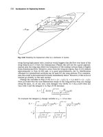
FIGURE 1.1
All of these vectors may be denoted A, since their magnitudes and directions are the same.


1.2 VECTORS
A vector is an object that is specified by both a magnitude and a direction. We represent a vector graphically by a directed line segment, that is, an arrow pointing in the direction of the vector. The end opposite
the arrow is called the tail. The length of the arrow is proportional to the magnitude of the vector. Velocity
is a good example of a vector. We say that a car is traveling east at eighty kilometers per hour. The direction
is east and the magnitude, or speed, is 80 km/h. We will use boldface type to represent vector quantities and
plain type to denote scalars. Thus, whereas B is a scalar, B is a vector.
Observe that a vector is specified solely by its magnitude and direction. If A is a vector, then all vectors
having the same physical dimensions, the same length and pointing in the same direction as A are denoted
A, regardless of their line of action, as illustrated in Figure 1.1. Shifting a vector parallel to itself does not
mathematically change the vector. However, parallel shift of a vector might produce a different physical
effect. For example, an upward 5 kN load (force vector) applied to the tip of an airplane wing gives rise to
quite a different stress and deflection pattern in the wing than the same load acting at the wing’s mid-span.
The magnitude of a vector A is denoted A , or, simply A.
Multiplying a vector B by the reciprocal of its magnitude produces a vector which points in the direction
of B, but it is dimensionless and has a magnitude of one. Vectors having unit dimensionless magnitude are
called unit vectors. We put a hat (^ ) over the letter representing a unit vector. Then we can tell simply by
ˆ and eˆ .
inspection that, for example, uˆ is a unit vector, as are B
It is convenient to denote the unit vector in the direction of the vector A as uˆ A . As pointed out above, we
obtain this vector from A as follows
uˆ A ϭ

A
A

(1.1)

Likewise, uˆ C ϭ C/C , uˆ F ϭ F/F , etc.
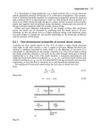
The sum or resultant of two vectors is defined by the parallelogram rule (Figure 1.2). Let C be the sum

of the two vectors A and B. To form that sum using the parallelogram rule, the vectors A and B are shifted
parallel to themselves (leaving them unaltered) until the tail of A touches the tail of B. Drawing dotted lines
through the head of each vector parallel to the other completes a parallelogram. The diagonal from the tails
of A and B to the opposite corner is the resultant C. By construction, vector addition is commutative, that is,
AϩB ϭ BϩA

(1.2)

A Cartesian coordinate system in three dimensions consists of three axes, labeled x, y and z, which intersect at the origin O. We will always use a right-handed Cartesian coordinate system, which means if you
wrap the fingers of your right hand around the z axis, with the thumb pointing in the positive z direction,


1.2 Vectors

3

C

B
A

FIGURE 1.2
Parallelogram rule of vector addition.
k
z

Az
O

y


j

Ax

x
Ay

Axy

i

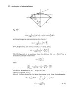
FIGURE 1.3
Three-dimensional, right-handed Cartesian coordinate system.

your fingers will be directed from the x axis towards the y axis. Figure 1.3 illustrates such a system. Note that
the unit vectors along the x, y and z-axes are, respectively, ˆi , ˆj and kˆ .
In terms of its Cartesian components, and in accordance with the above summation rule, a vector A is
written in terms of its components Ax , Ay and Az as
A ϭ Ax ˆi ϩ Ay ˆj ϩ Az kˆ

(1.3)

The projection of A on the xy plane is denoted A xy . It follows that
A xy ϭ Ax ˆi ϩ Ay ˆj
According to the Pythagorean theorem, the magnitude of A in terms of its Cartesian components is
Aϭ

Ax 2 ϩ Ay 2 ϩ Az 2


(1.4)

From Equations 1.1 and 1.3, the unit vector in the direction of A is
uˆ A ϭ cos θx ˆi ϩ cos θy ˆj ϩ cos θz kˆ

(1.5)


4

CHAPTER 1 Dynamics of point masses

k
z

Az
θx

A
θz
θy

Ax

j

y

y


x
i

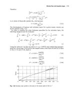
FIGURE 1.4
Direction angles in three dimensions.

where
cos θx ϭ

Ax
A

cos θy ϭ

Ay
A

cos θz ϭ

Az
A

(1.6)

The direction angles θx, θy and θz are illustrated in Figure 1.4, and are measured between the vector and the
positive coordinate axes. Note carefully that the sum of θx, θy and θz is not in general known a priori and
cannot be assumed to be, say, 180 degrees.
Example 1.1
Calculate the direction angles of the vector A ϭ ˆi Ϫ 4 ˆj ϩ 8kˆ .
Solution

First, compute the magnitude of A by means of Equation 1.4:
A ϭ 12 ϩ (Ϫ4)2 ϩ 82 ϭ 9
Then Equations 1.6 yield
⎛A ⎞
⎛1⎞
θx ϭ cosϪ1 ⎜⎜ x ⎟⎟⎟ ϭ cosϪ1 ⎜⎜ ⎟⎟⎟ ⇒
⎜⎝ 9 ⎠
⎜⎝ A ⎠

θx ϭ 83.62Њ

⎛ Ay ⎞
⎛Ϫ4 ⎞
θy ϭ cosϪ1 ⎜⎜⎜ ⎟⎟⎟ ϭ cosϪ1 ⎜⎜ ⎟⎟⎟⇒
⎜⎝ 9 ⎠
⎟
⎜⎝ A ⎠

θy ϭ 116.4Њ

⎛A ⎞
⎛8⎞
θz ϭ cosϪ1 ⎜⎜ z ⎟⎟⎟ ϭ cosϪ1 ⎜⎜ ⎟⎟⎟ ⇒
⎜⎝ 9 ⎠
⎜⎝ A ⎟⎠

θz ϭ 27.27Њ

Observe that θx ϩ θy ϩ θz ϭ 227.3°.



1.2 Vectors

5

Multiplication and division of two vectors are undefined operations. There are no rules for computing
the product AB and the ratio A/B . However, there are two well-known binary operations on vectors: the
dot product and the cross product. The dot product of two vectors is a scalar defined as follows,
A · B ϭ AB cosθ

(1.7)

where θ is the angle between the heads of the two vectors, as shown in Figure 1.5. Clearly,
AиB ϭ Bи A

(1.8)

If two vectors are perpendicular to each other, then the angle between them is 90°. It follows from
Equation 1.7 that their dot product is zero. Since the unit vectors ˆi , ˆj and kˆ of a Cartesian coordinate system are mutually orthogonal and of magnitude one, Equation 1.7 implies that
ˆi и ˆi ϭ ˆj и ˆj ϭ kˆ и kˆ ϭ 1
ˆi и ˆj ϭ ˆi и kˆ ϭ ˆj и kˆ ϭ 0

(1.9)

Using these properties it is easy to show that the dot product of the vectors A and B may be found in terms
of their Cartesian components as
A и B ϭ Ax Bx ϩ Ay By ϩ Az Bz

(1.10)


If we set B ϭ A, then it follows from Equations 1.4 and 1.10 that
Aϭ

AиA

(1.11)

The dot product operation is used to project one vector onto the line of action of another. We can imagine bringing the vectors tail to tail for this operation, as illustrated in Figure 1.6. If we drop a perpendicular
B
A
θ

FIGURE 1.5
The angle between two vectors brought tail to tail by parallel shift.
B
uA
θ
BA

FIGURE 1.6
Projecting the vector B onto the direction of A.

A


6

CHAPTER 1 Dynamics of point masses

line from the tip of B onto the direction of A, then the line segment BA is the orthogonal projection of B

onto line of action of A. BA stands for the scalar projection of B onto A. From trigonometry, it is obvious
from the figure that
BA ϭ B cosθ
Let uˆ A be the unit vector in the direction of A . Then
1

B и uˆ A ϭ B uˆ A cos θ ϭ B cos θ
Comparing this expression with the preceding one leads to the conclusion that
BA ϭ B и uˆ A ϭ B и

A
A

(1.12)

where uˆ A is given by Equation 1.1. Likewise, the projection of A onto B is given by
AB ϭ A и

B
B

Observe that AB ϭ BA only if A and B have the same magnitude.
Example 1.2
Let A ϭ ˆi ϩ 6 ˆj ϩ 18kˆ and B ϭ 42 ˆi Ϫ 69ˆj ϩ 98kˆ . Calculate
(a) The angle between A and B;
(b) The projection of B in the direction of A;
(c) The projection of A in the direction of B.
Solution
First we make the following individual calculations.
A и B ϭ (1)(42) ϩ (6)(Ϫ69) ϩ (18)(98) ϭ 1392


(a)

A ϭ (1)2 ϩ (6)2 ϩ (18)2 ϭ 19

(b)

B ϭ (42)2 ϩ (Ϫ69)2 ϩ (98)2 ϭ 127

(c)

(a) According to Equation 1.7, the angle between A and B is
⎛ A и B ⎞⎟
θ ϭ cosϪ1 ⎜⎜
⎜⎝ AB ⎟⎟⎠
Substituting (a), (b) and (c) yields
⎛ 1392 ⎞⎟
⎟ ϭ 54.77Њ
θ ϭ cosϪ1 ⎜⎜
⎜⎝19 и 127 ⎟⎟⎠


1.2 Vectors

7

(b) From Equation 1.12 we find the projection of B onto A:
BA ϭ B и

A

AиB
ϭ
A
A

Substituting (a) and (b) we get
BA ϭ

1392
= 73.26
19

(c) The projection of A onto B is
AB ϭ A и

B
AиB
ϭ
B
B

Substituting (a) and (c) we obtain
AB ϭ

1392
ϭ 10.96
127

The cross product of two vectors yields another vector, which is computed as follows,


ˆ AB
A ϫ B ϭ (ABsin θ ) n

(1.13)

where θ is the angle between the heads of A and B, and nˆ AB is the unit vector normal to the plane defined by
the two vectors. The direction of nˆ AB is determined by the right hand rule. That is, curl the fingers of the right
hand from the first vector (A) towards the second vector (B), and the thumb shows the direction of nˆ AB. See
Figure 1.7. If we use Equation 1.13 to compute B ϫ A, then nˆ AB points in the opposite direction, which means
B ϫ A ϭ Ϫ( A ϫ B)

(1.14)

Therefore, unlike the dot product, the cross product is not commutative.
The cross product is obtained analytically by resolving the vectors into Cartesian components.
A ϫ B ϭ (Ax ˆi ϩ Ay ˆj ϩ Az kˆ ) ϫ (Bx ˆi ϩ By ˆj ϩ Bz kˆ )

(1.15)

Since the set ˆˆ
ijkˆ is a mutually perpendicular triad of unit vectors, Equation 1.13 implies that
ˆi ϫ ˆi ϭ 0
ˆi ϫ ˆj ϭ kˆ
nAB

ˆj ϫ ˆj ϭ 0
ˆj ϫ kˆ ϭ ˆi

kˆ ϫ kˆ ϭ 0
kˆ ϫ ˆi ϭ ˆj


B
θ

A

FIGURE 1.7

nˆ AB is normal to both A and B and defines the direction of the cross product A ϫ B.

(1.16)


8

CHAPTER 1 Dynamics of point masses

Expanding the right side of Equation 1.15, substituting Equation 1.16 and making use of Equation 1.14
leads to
A ϫ B ϭ (Ay Bz Ϫ Az By )ˆi Ϫ (Ax Bz Ϫ Az Bx )ˆj ϩ (Ax By Ϫ Ay Bx )kˆ

(1.17)

It may be seen that the right-hand side is the determinant of the matrix
⎡ ˆi
ˆj
kˆ ⎤⎥
⎢
⎢A A A ⎥
y

z⎥
⎢ x
⎢
⎥
⎢⎢ Bx By Bz ⎥⎥
⎣
⎦
Thus, Equation 1.17 can be written
ˆi
A ϫ B ϭ Ax

ˆj
Ay

kˆ
Az

Bx

By

Bz

(1.18)

where the two vertical bars stand for determinant. Obviously the rule for computing the cross product,
though straightforward, is a bit lengthier than that for the dot product. Remember that the dot product yields
a scalar whereas the cross product yields a vector.
The cross product provides an easy way to compute the normal to a plane. Let A and B be any two vectors lying in the plane, or, let any two vectors be brought tail-to-tail to define a plane, as shown in Figure
1.7. The vector C ϭ A ϫ B is normal to the plane of A and B. Therefore, nˆ AB ϭ C/C , or

n AB ϭ

AϫB
AϫB

(1.19)

Example 1.3
Let A ϭ Ϫ3ˆi ϩ 7ˆj ϩ 9kˆ and B ϭ 6 ˆi Ϫ 5ˆj ϩ 8kˆ . Find a unit vector that lies in the plane of A and B and is
perpendicular to A.
Solution
The plane of the vectors A and B is determined by parallel shifting the vectors so that they meet tail to tail.
Calculate the vector D ϭ A ϫ B.
ˆi
ˆj kˆ
D ϭ Ϫ3 7 9 ϭ 101ˆi ϩ 78ˆj Ϫ 27kˆ
6 Ϫ5 8
Note that A and B are both normal to D. We next calculate the vector C ϭ D ϫ A.
ˆi
ˆj
kˆ
C ϭ 101 78 Ϫ27 ϭ 891ˆi Ϫ 828ˆj ϩ 941kˆ
Ϫ3 7
9