SPECTROSCOPY FOR THE BIOLOGICAL SCIENCESS
Bạn đang xem bản rút gọn của tài liệu. Xem và tải ngay bản đầy đủ của tài liệu tại đây (2.85 MB, 184 trang )
SPECTROSCOPY FOR
THE BIOLOGICAL
SCIENCES
Spectroscopy for the Biological Sciences, by Gordon G. Hammes
Copyright © 2005 John Wiley & Sons, Inc.
SPECTROSCOPY FOR
THE BIOLOGICAL
SCIENCES
GORDON G. HAMMES
Department of Biochemistry
Duke University
A JOHN WILEY & SONS, INC., PUBLICATION
Copyright © 2005 by John Wiley & Sons, Inc. All rights reserved
Published by John Wiley & Sons, Inc., Hoboken, New Jersey
Published simultaneously in Canada
No part of this publication may be reproduced, stored in a retrieval system, or transmitted in
any form or by any means, electronic, mechanical, photocopying, recording, scanning, or
otherwise, except as permitted under Section 107 or 108 of the 1976 United States Copyright
Act, without either the prior written permission of the Publisher, or authorization through
payment of the appropriate per-copy fee to the Copyright Clearance Center, Inc., 222
Rosewood Drive, Danvers, MA 01923, (978) 750-8400, fax (978) 750-4470, or on the web at
www.copyright.com. Requests to the Publisher for permission should be addressed to the
Permissions Department, John Wiley & Sons, Inc., 111 River Street, Hoboken, NJ 07030,
(201) 748-6011, fax (201) 748-6008, or online at />Limit of Liability/Disclaimer of Warranty: While the publisher and author have used their best
efforts in preparing this book, they make no representations or warranties with respect to the
accuracy or completeness of the contents of this book and specifically disclaim any implied
warranties of merchantability or fitness for a particular purpose. No warranty may be created
or extended by sales representatives or written sales materials. The advice and strategies
contained herein may not be suitable for your situation. You should consult with a professional
where appropriate. Neither the publisher nor author shall be liable for any loss of profit or any
other commercial damages, including but not limited to special, incidental, consequential, or
other damages.
For general information on our other products and services or for technical support, please
contact our Customer Care Department within the United States at (800) 762-2974, outside the
United States at (317) 572-3993 or fax (317) 572-4002.
Wiley also publishes its books in a variety of electronic formats. Some content that appears in
print may not be available in electronic formats. For more information about Wiley products,
visit our web site at www.wiley.com.
Library of Congress Cataloging-in-Publication Data:
Hammes, Gordon G., 1934–
Spectroscopy for the biological sciences / Gordon G. Hammes.
p. ; cm.
Companion v. to: Thermodynamics and kinetics for the biological sciences /
Gordon G. Hammes. c2000.
Includes bibliographical references and index.
ISBN-13 978-0-471-71344-9 (pbk.)
ISBN-10 0-471-71344-9 (pbk.)
1. Biomolecules—Spectra. 2. Spectrum analysis.
[DNLM: 1. Spectrum Analysis. 2. Crystallography, X-Ray. ] I. Hammes, Gordon G.,
1934– Thermodynamics and kinetics for the biological sciences. II. Title.
QP519. 9. S6H35 2005
572—dc22
2004028306
Printed in the United States of America
10
9
8
7
6
5
4
3
2
1
CONTENTS
PREFACE
ix
1.
1
FUNDAMENTALS OF SPECTROSCOPY
Introduction / 1
Quantum Mechanics / 3
Particle in a Box / 5
Properties of Waves / 9
References / 13
Problems / 14
2.
X-RAY CRYSTALLOGRAPHY
17
Introduction / 17
Scattering of X Rays by a Crystal / 18
Structure Determination / 22
Neutron Diffraction / 25
Nucleic Acid Structure / 25
Protein Structure / 28
Enzyme Catalysis / 30
References / 32
Problems / 32
v
vi
3.
CONTENTS
ELECTRONIC SPECTRA
35
Introduction / 35
Absorption Spectra / 36
Ultraviolet Spectra of Proteins / 38
Nucleic Acid Spectra / 40
Prosthetic Groups / 41
Difference Spectroscopy / 44
X-Ray Absorption Spectroscopy / 46
Fluorescence and Phosphorescence / 47
RecBCD: Helicase Activity Monitored by Fluorescence / 51
Fluorescence Energy Transfer: A Molecular Ruler / 52
Application of Energy Transfer to Biological Systems / 54
Dihydrofolate Reductase / 57
References / 58
Problems / 59
4. CIRCULAR DICHROISM, OPTICAL ROTARY DISPERSION,
AND FLUORESCENCE POLARIZATION
63
Introduction / 63
Optical Rotary Dispersion / 65
Circular Dichroism / 66
Optical Rotary Dispersion and Circular Dichroism of Proteins / 67
Optical Rotation and Circular Dichroism of
Nucleic Acids / 69
Small Molecule Binding to DNA / 71
Protein Folding / 74
Interaction of DNA with Zinc Finger Proteins / 77
Fluorescence Polarization / 78
Integration of HIV Genome into Host Genome / 80
a-Ketoglutarate Dehyrogenase / 81
References / 84
Problems / 84
5.
VIBRATIONS IN MACROMOLECULES
Introduction / 89
Infrared Spectroscopy / 92
Raman Spectroscopy / 92
Structure Determination with Vibrational Spectroscopy / 95
89
CONTENTS
vii
Resonance Raman Spectroscopy / 98
Structure of Enzyme-Substrate Complexes / 100
References / 101
Problems / 102
6. PRINCIPLES OF NUCLEAR MAGNETIC RESONANCE AND
ELECTRON SPIN RESONANCE
103
Introduction / 103
NMR Spectrometers / 106
Chemical Shifts / 108
Spin-Spin Splitting / 110
Relaxation Times / 112
Multidimensional NMR / 115
Magnetic Resonance Imaging / 121
Electron Spin Resonance / 122
References / 125
Problems / 125
7. APPLICATIONS OF MAGNETIC RESONANCE TO
BIOLOGY
129
Introduction / 129
Regulation of DNA Transcription / 129
Protein-DNA Interactions / 132
Dynamics of Protein Folding / 133
RNA Folding / 136
Lactose Permease / 139
Conclusion / 142
References / 142
8.
MASS SPECTROMETRY
Introduction / 145
Mass Analysis / 145
Tandem Mass Spectrometry (MS/MS) / 149
Ion Detectors / 150
Ionization of the Sample / 150
Sample Preparation/Analysis / 154
Proteins and Peptides / 154
Protein Folding / 157
Other Biomolecules / 160
145
viii
CONTENTS
References / 161
Problems / 161
APPENDICES
1. Useful Constants and Conversion Factors / 163
2. Structures of the Common Amino Acids at Neutral pH / 165
3. Common Nucleic Acid Components / 167
INDEX
169
PREFACE
This book is intended as a companion to Thermodynamics and Kinetics for the
Biological Sciences, published in 2000. These two books are based on a course
that has been given to first-year graduate students in the biological sciences
at Duke University. These students typically do not have a strong background
in mathematics and have not taken a course in physical chemistry. The
intent of both volumes is to introduce the concepts of physical chemistry that
are of particular interest to biologists with a minimum of mathematics. I
believe that it is essential for all students in the biological sciences to feel comfortable with quantitative interpretations of the phenomena they are studying. Indeed, the necessity to be able to use quantitative concepts has become
even more important with recent advances, for example, in the fields of
proteomics and genomics. The two volumes can be used for a one-semester
introduction to physical chemistry at both the first-year graduate level and at
the sophomore-junior undergraduate level. As in the first volume, some problems are included, as they are necessary to achieve a full understanding of the
subject matter.
I have taken some liberties with the definition of spectroscopy so that chapters on x-ray crystallography and mass spectrometry are included in this
volume. This is because of the importance of these tools for understanding biological phenomena. The intent is to give students a fairly complete background
in the physical chemical aspects of biology, although obviously the coverage
cannot be as complete or as rigorous as a traditional two-semester course in
physical chemistry. The approach is more conceptual than traditional physical
chemistry, and many examples of applications to biology are presented.
I am indebted to my colleagues at Duke for their assistance in looking over
parts of the text and supplying material. Special thanks are due to Professors
ix
x
PREFACE
David Richardson, Lorena Beese, Leonard Spicer, Terrence Oas, and Michael
Fitzgerald. I again thank my wife, Judy, who has encouraged, assisted, and
tolerated this effort. I welcome comments and suggestions from readers.
Gordon G. Hammes
CHAPTER 1
FUNDAMENTALS OF SPECTROSCOPY
INTRODUCTION
Spectroscopy is a powerful tool for studying biological systems. It often
provides a convenient method for analysis of individual components in a
biological system such as proteins, nucleic acids, and metabolites. It can also
provide detailed information about the structure and mechanism of action of
molecules. In order to obtain the maximum benefit from this tool and to use
it properly, a basic understanding of spectroscopy is necessary. This includes
a knowledge of the fundamentals of spectroscopic phenomena, as well as
of the instrumentation currently available. A detailed understanding involves
complex theory, but a grasp of the important concepts and their application
can be obtained without resorting to advanced mathematics and theory. We
will attempt to do this by emphasizing the physical ideas associated with
spectral phenomena and utilizing a few of the concepts and results from
molecular theory.
Very simply stated, spectroscopy is the study of the interaction of radiation
with matter. Radiation is characterized by its energy, E, which is linked to
the frequency, u, or wavelength, l, of the radiation by the familiar Planck
relationship:
E = hu = hc l
(1-1)
Spectroscopy for the Biological Sciences, by Gordon G. Hammes
Copyright © 2005 John Wiley & Sons, Inc.
1
2
FUNDAMENTALS OF SPECTROSCOPY
where c is the speed of light, 2.998 ¥ 1010 cm/s (2.998 ¥ 108 m/s), and h is Planck’s
constant, 6.625 ¥ 10-27 erg-s (6.625 ¥ 10-34 J-s). Note that lu = c.
Radiation can be envisaged as an electromagnetic sine wave that contains
both electric and magnetic components, as shown in Figure 1-1. As shown in
the figure, the electric component of the wave is perpendicular to the magnetic component. Also shown is the relationship between the sine wave and
the wavelength of the light. The useful wavelength of radiation for spectroscopy extends from x-rays, l ~ 1–100 nm, to microwaves, l ~ 105–106 nm. For
biology, the most useful radiation for spectroscopy is in the ultraviolet and
visible region of the spectrum. The entire useful spectrum is shown in Figure
1-2, along with the common names for the various regions of the spectrum. If
Z
magnetic field
X
l
electric field
Y
Figure 1-1. Schematic representation of an electromagnetic sine wave. The electric
field is in the xz plane and the magnetic field in the xy plane. The electric and magnetic
fields are perpendicular to each other at all times. The wavelength, l, is the distance
required for the wave to go through a complete cycle.
HIGH ENERGY
g rays
x rays
10-3
10-1
LOW ENERGY
uv vis
10
ir
103
microwaves
105
107
radiowaves
109
1011
Wavelength (nm)
Figure 1-2. Schematic representation of the wavelengths associated with electromagnetic radiation. The wavelengths, in nanometers, span 14 orders of magnitude. The
common names of the various regions also are indicated approximately (uv is ultraviolet; vis is visible; and ir is infrared).
QUANTUM MECHANICS
3
radiation is envisaged as both an electric and magnetic wave, then its interactions with matter can be considered as electromagnetic phenomena, due to
the fact that matter is made up of positive and negative charges. We will not
be concerned with the details of this interaction, which falls into the domain
of quantum mechanics. However, a few of the basic concepts of quantum
mechanics are essential for understanding spectroscopy.
QUANTUM MECHANICS
Maximum kinetic energy
of emitted electron
Quantum mechanics was developed because of the failure of Newtonian
mechanics to explain experimental results that emerged at the beginning of
the 20th century. For example, for certain metals (e.g., Na), electrons are
emitted when light is absorbed. This photoelectric effect has several nonclassical characteristics. First, for light of a given frequency, the kinetic energy of
the electrons emitted is independent of the light intensity. The number of electrons produced is proportional to the light intensity, but all of the electrons
have the same kinetic energy. Second, the kinetic energy of the photoelectron
is zero until a threshold energy is reached, and then the kinetic energy
becomes proportional to the frequency. This behavior is shown schematically
in Figure 1-3, where the kinetic energy of the electrons is shown as a function
n0
Ø
n, s-1
Figure 1-3. Schematic representation of the photoelectric effect. The maximum kinetic
energy of an electron emitted from a metal surface when it is illuminated with light of
frequency u is shown. The frequency at which electrons are no longer emitted determines the work function, hu0, and the slope of the line is Planck’s constant (Eq. 1-2).
4
FUNDAMENTALS OF SPECTROSCOPY
of the frequency of the radiation. An explanation of these phenomena was
proposed by Einstein, who, following Planck, postulated that energy is
absorbed only in discrete amounts of energy, hu. A photon of energy hu has
the possibility of ejecting an electron, but a minimum energy is necessary.
Therefore,
Kinetic Energy = hu - hu 0
(1-2)
where hu0 is the work function characteristic of the metal. This predicts that
altering the light intensity would affect only the number of photoelectrons
and not the kinetic energy. Furthermore, the slope of the experimental plot
(Fig. 1-3) is h.
This explanation of the photoelectric effect postulates that light is corpuscular and consists of discrete photons characterized by a specific frequency.
How can this be reconciled with the well-known wave description of light
briefly discussed above? The answer is that both descriptions are correct—
light can be envisioned either as discrete photons or a continuous wave. This
wave-particle duality is a fundamental part of quantum mechanics. Both
descriptions are correct, but one of them may more easily explain a given
experimental situation.
About this point in history, de Broglie suggested this duality is applicable
to matter also, so that matter can be described as particles or waves. For light,
the energy is equal to the momentum, p, times the velocity of light, and by
Einstein’s postulate is also equal to hu.
E = hu = pc
(1-3)
Furthermore, since lu = c, p = h/l. For macroscopic objects, p = mv, where
v is the velocity and m is the mass. In this case, l = h/(mv), the de Broglie
wavelength. These fundamental relationships have been verified for matter
by several experiments such as the diffraction of electrons by crystals. The
postulate of de Broglie can be extended to derive an important result of
quantum mechanics developed by Heisenberg in 1927, namely the uncertainty
principle:
Dp Dx ≥ h (2 p)
(1-4)
In this equation, Dp represents the uncertainty in the momentum and Dx the
uncertainty in the position. The uncertainty principle means that it is not possible to determine the precise values of the momentum, p, and the position, x.
The more precisely one of these variables is known, the less precisely the other
variable is known. This has no practical consequences for macroscopic systems
but is crucial for the consideration of systems at the atomic level. For example,
if a ball weighing 100 grams moves at a velocity of 100 miles per hour (a good
tennis serve), an uncertainty of 1 mile per hour in the speed gives Dp ~ 4.4 ¥
PARTICLE IN A BOX
5
10-2 kg m/sec and Dx ~ 2 ¥ 10-33 m. We are unlikely to worry about this uncertainty! On the other hand, if an electron (mass = 9 ¥ 10-28 g) has an uncertainty
in its velocity of 1 ¥ 108 cm/sec, the uncertainty in the position is about 1 Å, a
large distance in terms of atomic dimensions. As we will see later, quantum
mechanics has an alternative way of defining the position of an electron.
A second puzzling aspect of experimental physics in the late 1800s and early
1900s was found in the study of atomic spectra. Contrary to the predictions of
classical mechanics, discrete lines at specific frequencies were observed when
atomic gases at high temperatures emitted radiation. This can only be understood by the postulation of discrete energy levels for electrons. This was first
explained by the famous Bohr atom, but this model was found to have shortcomings, and the final resolution of the problem occurred only when quantum
mechanics was developed by Schrödinger and Heisenberg in the late 1920s.
We will only consider the development by Schrödinger, which is somewhat
less complex than that of Heisenberg.
Schrödinger postulated that all matter can be described as a wave and
developed a differential equation that can be solved to determine the properties of a system. Basically, this differential equation contains two important
variables, the kinetic energy and the potential energy. Both of these are wellknown concepts from classical mechanics, but they are redefined in the development of quantum mechanics. If the wave equation is solved for specific
systems, it fully explains the previously puzzling results. Energy is quantized,
so discrete energy levels are obtained. Furthermore, a consequence of
quantum mechanics is that the position of a particle can never be completely
specified. Instead, the probability of finding a particle in a specific location can
be determined, and the average position of a particle can be calculated. This
probabilistic view of matter is in contrast to the deterministic character of
Newtonian mechanics and has sparked considerable philosophic debate. In
fact, Einstein apparently never fully accepted this probabilistic view of nature.
In addition to the above concepts, quantum mechanics also permits quantitative calculations of the interaction of radiation with matter. The result is the
specification of rules that ultimately determine what is observed experimentally. We will make use of these rules without considering the details of their
origin, but it is important to remember that they stem from detailed quantum
mechanical calculations.
PARTICLE IN A BOX
As an example of a simple quantum mechanical result that leads to quantization of energy levels, we consider a particle of mass m moving back and forth
in a one-dimensional box of length L. This actually has some practical application. It is a good model for the movement of pi electrons that are delocalized over a large part of a molecule, for example, biological molecules such as
carotenoids, hemes, and chlorophyll. This is not an ordinary box because inside
6
FUNDAMENTALS OF SPECTROSCOPY
U=•
U=•
U=0
O
X
L
Figure 1-4. Quantum mechanical model for a particle in a one-dimensional box of
length L. The particle is confined to the box by setting the potential energy equal to 0
inside the box and to • outside of the box.
the box, the potential energy of the system is 0, whereas outside of the box,
the potential energy is infinite. This is depicted in Figure 1-4. The Schrödinger
equation in one dimension is
-
h2 d 2y n
+ U = En yn
8 mp 2 dx 2
(1-5)
where Yn is the wave function, x is the position coordinate, U is the potential
energy, and En is the energy associated with the wave function Yn. Since the
potential walls are infinitely high, the solution to this equation outside of the
box is easy—there is no chance the particle is outside the box so the wave
function must be 0. Inside the box, U = 0, and Eq. 1-5 can be easily solved. The
solution is
y n = A sinbx
(1-6)
where A and b are constants. At the ends of the box, Y must be zero. This
happen when sin np = 0 and n is an integer, so b must be equal to np/L. This
causes Yn to be 0 when x = 0 and x = L for all integral values of n. To evaluate A, we introduce another concept from quantum mechanics, namely that
the probability of finding the particle in the interval between x and x + dx
is Y2dx. Since the particle must be in the box, the probability of finding the
particle in the box is 1, or
L
L
Ú y n2 dx = Ú A 2 sin 2 (np x L)dx = 1
0
(1-7)
0
Evaluation of this integral gives A = 2 L Thus the final result for the wave
function is
y n = 2 L sin(npx L)
(1-8)
PARTICLE IN A BOX
O
X
3
y3 = 2 / L sin (3p x / L )
2
y2 = 2 / L sin (2p x / L )
1
y1 = 2 / L sin (p x / L )
7
L
Figure 1-5. Wave functions, Y, for the first three energy levels of the particle in a box
(Eq. 1-8). The dashed lines show the probability of the finding the particle at a given
position x, Y2.
Obviously n cannot be 0, as this would predict that there is no probability of
finding the particle in the box, but n can be any integer. The wave functions
for a few values of n are shown in Figure 1-5. Basically Yn is a sine wave, with
the “wavelength” decreasing as n increases. (More advanced treatments of
quantum mechanics use the notation associated with complex numbers in discussing the wave equation and wave functions, but this is beyond the scope of
this text.)
To determine the energy of the particle, all we have to do is put Eq. 1-8
back into Eq. 1-5 and solve for En. The result is
E n = (h 2 n 2 ) (8 mL2 )
(1-9)
Thus, we see that the energy is quantized, and the energy is characterized by
a series of energy levels, as depicted in Figure 1-6. Each energy level, En, is
associated with a specific wave function, Yn. Notice that the energy levels
would be very widely spaced for a very light particle such as an electron, but
would be very closely spaced for a macroscopic particle. Similarly, the smaller
the box, the more widely spaced the energy levels. For a tennis ball being hit
on a tennis court, the ball is sufficiently heavy and the court (box) sufficiently
big so that the energy levels would be a continuum for all practical purposes.
The uncertainty in the momentum and position of the ball cannot be blamed
on quantum mechanics in this case! The particle in a box illustrates how
quantum mechanics can be used to calculate the properties of systems and
how quantization of energy levels arises. The same calculation can be easily
done for a three-dimensional box. In this case, the energy states are the sum
8
FUNDAMENTALS OF SPECTROSCOPY
25 E1
n =5
Energy
16 E1
n =4
9 E1
n =3
4 E1
n =2
E1
n =1
Figure 1-6. Energy levels for a particle in a box (Eq. 1-9). The energy levels are n2E1
where E1 is the energy when n = 1.
of three terms identical to Eq. 1-9, but with each of the three terms having a
different quantum number.
The quantum mechanical description of matter does not permit determination of the precise position of the particle to be determined, a manifestation of the Heisenberg uncertainty principle. However, the probability of
finding the particle within a given segment of the box can be calculated. For
example, the probability of finding the particle in the middle of the box, that
is, between L/4 and 3L/4 for the lowest energy state is
3L 4
Ú
L 4
3L 4
y 12 dx = (2 L)
Ú
sin 2 (p x L)dx
L 4
Evaluation of this integral gives a probability of 0.82.The probability of finding
the particle within the middle part of the box is independent of L, the size of
the box, but does depend on the value of the quantum number, n. For the
second energy level, n = 2, the probability is 0.50. The probability of finding
the particle at position x in the box is shown as a dashed line for the first three
energy levels in Figure 1-5.
An important result of quantum mechanics is that not only do molecules
exist in different discrete energy levels, but the interaction of radiation with
molecules causes shifts between these energy levels. If energy or radiation is
absorbed by a molecule, the molecule can be raised to a higher energy state,
whereas if a molecule loses energy, radiation can be emitted. For both cases,
the change in energy is related to the radiation that is absorbed or emitted by
a slight modification of Eq. 1-1, namely the change in energy state of the molecule, DE, is
PROPERTIES OF WAVES
DE = hu = hc l
9
(1-10)
The change in energy, DE, is the difference in energy between specific energy
levels of the molecule, for example, E2 - E1 where 1 and 2 designate different
energy levels. It is important to note that since the energy is quantized, the
light emitted or absorbed is always a specific single frequency. Equation 1-10
can be applied to the particle in a box for the particle dropping from the
n + 1 energy level to the n energy level:
DE =
h2
h2
2
2 =
(
)
(2 n + 1) = hc l
n
+
1
n
8 mL2
8 mL2
[
]
(1-11)
If the particle is assumed to be an electron moving in a molecule 20 Å long
and n = 10, then l ~ 600 nm. This wavelength is in the visible region and has
been observed for p electrons that are highly delocalized in molecules.
In practice, energy levels are sometimes so closely spaced that the frequencies of light emitted appear to create a continuum of frequencies. This is
a shortcoming of the experimental method—in reality the frequencies emitted
are discrete entities. The particle in a box is a rather simple application of
quantum mechanics, but it illustrates several important points that also are
found in more complex calculations for molecular systems. First, the system
can be described by a wave function. Second, this wave function permits determination of the probability of important characteristics of the system, such as
positions. Finally, the energy of the system can be calculated and is found to
be quantized. Moreover, the energy can only be absorbed or emitted in quantized packages characterized by specific frequencies. Quantum mechanical calculations also tell us what conditions are necessary for energy to be emitted
or absorbed by a molecule. These calculations tell us whether radiation will be
emitted or absorbed and what quantized packets of energy are available. We
will only utilize the results of these calculations and will not be concerned with
the details of the interactions between light and molecules other than the
above concepts.
PROPERTIES OF WAVES
It is useful to consider several additional aspects of light waves in order to
understand better some of the experimental methods that will be discussed
later. Thus far we have considered light to be a periodic electromagnetic wave
in space that could be characterized, for example, by a sine function:
I = I 0 sin(2 px l)
(1-12)
Here I is the magnetic or electric field, I0 is the maximum value of the electric or magnetic field, x is the distance along the x axis and l is the wavelength.
10
FUNDAMENTALS OF SPECTROSCOPY
A light wave can also be periodic in time, as illustrated in Figure 1-7. In this
case:
I = I 0 sin 2 put = I 0 sin wt
(1-13)
Now, I is the light intensity, I0 is the maximum light intensity, u is the frequency
in s-1, as defined in Figure 1-7, w is the frequency in radians (w = 2pu), and t
is the time. The velocity of the propagating wave is lu, which in the case of
electromagnetic radiation is the speed of light, that is, lu = c. If light of the
same frequency and maximum amplitude from two sources is combined, the
two sine functions will be added. If the two light waves start with zero intensity at the same time (t = 0), the two waves add and the intensity is doubled.
This is called constructive interference. If the two waves are combined with one
of the waves starting at zero intensity and proceeding to positive values of the
sine function, whereas the other begins at zero intensity and proceeds to negative values, the two intensities cancel each other out. This is called destructive interference. Obviously it is possible to have cases in between these two
extremes. In such cases, a phase difference is said to exist between the two
waves. Mathematically this can be represented as
A
A+B
Amplitude
B
1/n
A
A+B
B
Time
Figure 1-7. Examples of constructive and destructive interference. Constructive interference: when the upper two wave forms of equal amplitude and a phase angle of 0°
(or integral multiples of 2p) are added (left), a sine wave with twice the amplitude and
the same frequency results (right). Destructive interference: when the lower two wave
forms are added (left), the amplitudes of the two waves cancel (right). The phase angle
in this case is 90° (or odd integral multiples of p/2).
PROPERTIES OF WAVES
I = I 0 sin(wt + d)
11
(1-14)
where d is called a phase angle and can be either positive or negative. When
many different waves of the same frequency are combined, the intensity can
always be described by such a relationship. These phenomena are shown
schematically in Figure 1-7.
A standard way of carrying out spectroscopy is to apply continuous radiation, and then look at the intensity of the radiation after it has passed through
the sample of interest. The intensity is then determined as a function of the
frequency of the radiation, and the result is the absorption spectrum of the
sample. The color of a material is determined by the wavelength of the light
absorbed. For example, if white light shines on blood, blue/green light is
absorbed so that the transmitted light is red. Several examples of absorption
spectra are shown in Figure 1-8. We will consider why and how much the
sample absorbs light a bit later, but you are undoubtedly already familiar with
the concept of an absorption spectrum.
The use of continuous radiation is a useful way to carry out an experiment,
but there is an interesting mathematical relationship that permits a different
approach to the problem. This mathematical operation is the Fourier transform. The principle of a Fourier transform is that if the frequency dependence
of the intensity, I(u), can be determined, it can be transformed into a new function, F(t), that is a function of the time, t. Conversely, F(t) can also be converted to I(u). Both of these functions contain the same information. Why then
are these transformations advantageous? It can be quite time consuming to
determine I(u), but a short pulse of radiation can be applied very quickly. Basically what this transformation means is that looking at the response of the
system to application of a pulse of radiation, such as shown as in Figure 1-9,
is equivalent to looking at the response of the system to sine wave radiation
at many different frequencies. In other words, a square wave is mathematically
equivalent to adding up many sine waves of different frequency, and vice versa.
This is shown schematically in Figure 1-9 where the addition of sine waves
with four different frequencies produces a periodic “square” wave. The larger
the number of sine waves added, the more “square” the wave becomes. In
mathematical terms, a square wave can be represented as an infinite series of
sine functions, a Fourier series.
The mathematical equivalence of timed pulses and continuous waves of
many different frequencies has profound consequences in determining the
spectroscopic properties of materials. In many cases, the use of pulses permits
thousands of experiments to be done in a very short time. The results of these
experiments can then be averaged, producing a far superior frequency spectrum in a much shorter time than could be determined by continuous wave
methods. In later chapters, we will be dealing both with continuous wave spectroscopy and Fourier transform spectroscopy. It is important to remember that
12
FUNDAMENTALS OF SPECTROSCOPY
Chlorophyll a
400
500
600
700
Absorbance
E.coli DNA
180
200
220
240
260
280
300
320
Oxyhemoglobin (Fe2+)
350
400
450
500
550
600
l (nm)
Figure 1-8. Absorption of light by biological molecules. The absorbance scale is arbitrary and the wavelength, l, is in nanometers. Chlorophyll a solutions absorb blue and
red light and are green in color. DNA solutions absorb light in the ultraviolet and are
colorless. Oxyhemoglobin solutions absorb blue light and are red in color.
both methods give identical results. The method of choice is that one that
produces the best data in the shortest time, and in some cases at the lowest
cost.
With this brief introduction to the underlying theoretical principles of
spectroscopy, we are ready to proceed with consideration of specific types of
spectroscopy and their application to biological systems.
13
Amplitude
REFERENCES
Time
Figure 1-9. The upper part of the figure shows sine waves of four different frequencies, and the lower part of the figure is the sum of the sine waves, which approximates
a square wave pulse of radiation. When sine waves of many more frequencies are
included, the time dependence becomes a pulsed square wave. This figure illustrates
that the superposition of multiple sine waves is equivalent to a square wave pulse and
vice versa. This equivalency is the essence of Fourier transform methods. Copyright by
Professor T. G. Oas, Duke University. Reproduced with permission.
REFERENCES
The topics in this chapter are discussed in considerably more depth in a number of
physical chemistry textbooks, such as those cited below.
1. I. Tinoco Jr., K. Sauer, J. C. Wang, and J. D. Puglisi, Physical Chemistry: Principles
and Applications in Biological Sciences, 4th edition, Prentice Hall, Englewood, NJ,
2002.
2. R. J. Silbey, R. A. Alberty, and M. G. Bawendi, Physical Chemistry, 4th edition, John
Wiley & Sons, New York, 2004.
14
FUNDAMENTALS OF SPECTROSCOPY
3. P. W. Atkins and J. de Paula, Physical Chemistry, 7th edition, W. H. Freeman, New
York, 2001.
4. R. S. Berry, S. A. Rice, and J. Ross, Physical Chemistry, 2nd edition, Oxford University Press, New York, 2000.
5. D. A. McQuarrie and J. D. Simon, Physical Chemistry: A Molecular Approach,
University Science Books, Sausalito, CA, 1997.
PROBLEMS
1.1. The energies required to break the C–C bond in ethane, the “triple bond”
in CO, and a hydrogen bond are about 88, 257, and 4 kcal/mol. What wavelengths of radiation are required to break these bonds?
1.2. Calculate the energy and momentum of a photon with the following
wavelengths: 150 pm (x ray), 250 nm (ultraviolet), 500 nm (visible), and
1 cm (microwave).
1.3. The maximum kinetic energy of electrons emitted from Na at different
wavelengths was measured with the following results.
l (Å)
4500
4000
3500
3000
Max Kinetic Energy (electron volts)
0.40
0.76
1.20
1.79
Calculate Planck’s constant and the value of the work function from these
data. (1 electron volt = 1.602 ¥ 10-19 J)
1.4. Calculate the de Broglie wavelength for the following cases:
a. An electron in an electron microscope accelerated with a potential of
100 kvolts.
b. A He atom moving at a speed of 1000 m/s.
c. A bullet weighing 1 gram moving at a speed of 100 m/s.
Assume the uncertainty in the speed is 10%, and calculate the uncertainty
in the position for each of the three cases.
1.5. The particle in a box is a useful model for electrons that can move
relatively freely within a bonding system such as p electrons. Assume an
electron is moving in a “box” that is 50 Å long, that is, a potential well
with infinitely high walls at the boundaries.
a. Calculate the energy levels for n = 1, 2, and 3.
b. What is the wavelength of light emitted when the electron moves from
the energy level with n = 2 to the energy level with n = 1?
PROBLEMS
15
c. What is the probability of finding the electron between 12.5 and 37.5
Å for n = 1.
1.6. Sketch the graph of I versus t for sine wave radiation that obeys the relationship I = I0sin (wt + d) for d = 0, p/4, p/2, and p.
Plot the sum of the sine waves when the sine wave for d = 0 is added to
that for d = 0 or p/4, or p/2, or p. This exercise should provide you with a
good understanding of constructive and destructive interference.
Do your results depend on the value of w? Briefly discuss what happens
when waves of different frequency are added together.