7708d_c03_100 8/10/01 3:01 PM Page 100 mac120 mac120:1st shift:

Flow past a blunt body: On any object placed in a moving fluid there is
a stagnation point on the front of the object where the velocity is zero.
This location has a relatively large pressure and divides the flow field
into two portions—one flowing over the body, and one flowing under
the body. 1Dye in water.2 1Photograph by B. R. Munson.2


7708d_c03_101 8/10/01 3:01 PM Page 101 mac120 mac120:1st shift:

3

Fluid
Elementary
Dynamics—The
Bernoulli Equation

The Bernoulli
equation may be
the most used and
abused equation in
fluid mechanics.

3.1

As was discussed in the previous chapter, there are many situations involving fluids in which
the fluid can be considered as stationary. In general, however, the use of fluids involves motion of some type. In fact, a dictionary definition of the word “fluid” is “free to change in
form.” In this chapter we investigate some typical fluid motions 1fluid dynamics2 in an elementary way.
To understand the interesting phenomena associated with fluid motion, one must consider the fundamental laws that govern the motion of fluid particles. Such considerations include the concepts of force and acceleration. We will discuss in some detail the use of Newton’s second law 1F ϭ ma2 as it is applied to fluid particle motion that is “ideal” in some
sense. We will obtain the celebrated Bernoulli equation and apply it to various flows. Although this equation is one of the oldest in fluid mechanics and the assumptions involved in

its derivation are numerous, it can be effectively used to predict and analyze a variety of flow
situations. However, if the equation is applied without proper respect for its restrictions, serious errors can arise. Indeed, the Bernoulli equation is appropriately called “the most used
and the most abused equation in fluid mechanics.”
A thorough understanding of the elementary approach to fluid dynamics involved in
this chapter will be useful on its own. It also provides a good foundation for the material in
the following chapters where some of the present restrictions are removed and “more nearly
exact” results are presented.

Newton’s Second Law
As a fluid particle moves from one location to another, it usually experiences an acceleration
or deceleration. According to Newton’s second law of motion, the net force acting on the fluid
particle under consideration must equal its mass times its acceleration,
F ϭ ma

101


7708d_c03_102 8/10/01 3:02 PM Page 102 mac120 mac120:1st shift:

102

■ Chapter 3 / Elementary Fluid Dynamics—The Bernoulli Equation

Inviscid fluid flow
in governed by
pressure and gravity forces.

In this chapter we consider the motion of inviscid fluids. That is, the fluid is assumed to have
zero viscosity. If the viscosity is zero, then the thermal conductivity of the fluid is also zero
and there can be no heat transfer 1except by radiation2.

In practice there are no inviscid fluids, since every fluid supports shear stresses when
it is subjected to a rate of strain displacement. For many flow situations the viscous effects
are relatively small compared with other effects. As a first approximation for such cases it
is often possible to ignore viscous effects. For example, often the viscous forces developed
in flowing water may be several orders of magnitude smaller than forces due to other influences, such as gravity or pressure differences. For other water flow situations, however, the
viscous effects may be the dominant ones. Similarly, the viscous effects associated with the
flow of a gas are often negligible, although in some circumstances they are very important.
We assume that the fluid motion is governed by pressure and gravity forces only and
examine Newton’s second law as it applies to a fluid particle in the form:
1Net pressure force on a particle2 ϩ 1net gravity force on particle2 ϭ
1particle mass2 ϫ 1particle acceleration2

The results of the interaction between the pressure, gravity, and acceleration provide numerous useful applications in fluid mechanics.
To apply Newton’s second law to a fluid 1or any other object2, we must define an appropriate coordinate system in which to describe the motion. In general the motion will be
three-dimensional and unsteady so that three space coordinates and time are needed to describe it. There are numerous coordinate systems available, including the most often used
rectangular 1x, y, z2 and cylindrical 1r, u, z2 systems. Usually the specific flow geometry dictates which system would be most appropriate.
In this chapter we will be concerned with two-dimensional motion like that confined
to the x–z plane as is shown in Fig. 3.1a. Clearly we could choose to describe the flow in
terms of the components of acceleration and forces in the x and z coordinate directions. The
resulting equations are frequently referred to as a two-dimensional form of the Euler equations of motion in rectangular Cartesian coordinates. This approach will be discussed in
Chapter 6.
As is done in the study of dynamics 1Ref. 12, the motion of each fluid particle is described in terms of its velocity vector, V, which is defined as the time rate of change of the
position of the particle. The particle’s velocity is a vector quantity with a magnitude 1the speed,
V ϭ 0 V 0 2 and direction. As the particle moves about, it follows a particular path, the shape
of which is governed by the velocity of the particle. The location of the particle along the
path is a function of where the particle started at the initial time and its velocity along the path.
If it is steady flow 1i.e., nothing changes with time at a given location in the flow field2, each
successive particle that passes through a given point [such as point 112 in Fig. 3.1a] will follow the same path. For such cases the path is a fixed line in the x–z plane. Neighboring par-

z


z

V
V (2)

n

Fluid particle

s

(1)

n=0
Streamlines
n = n1
᏾ = ᏾(s)

x
(a)

x
(b)

■ FIGURE 3.1

(a) Flow in the x–z plane.
(b) Flow in terms of
streamline and normal

coordinates.


7708d_c03_103 8/10/01 3:03 PM Page 103 mac120 mac120:1st shift:

3.1 Newton’s Second Law ■

Fluid particles accelerate normal to
and along streamlines.

103

ticles that pass on either side of point 112 follow their own paths, which may be of a different shape than the one passing through 112. The entire x–z plane is filled with such paths.
For steady flows each particle slides along its path, and its velocity vector is everywhere tangent to the path. The lines that are tangent to the velocity vectors throughout the
flow field are called streamlines. For many situations it is easiest to describe the flow in terms
of the “streamline” coordinates based on the streamlines as are illustrated in Fig. 3.1b. The
particle motion is described in terms of its distance, s ϭ s1t2, along the streamline from some
convenient origin and the local radius of curvature of the streamline, r ϭ r1s2. The distance along the streamline is related to the particle’s speed by V ϭ dsրdt, and the radius of
curvature is related to shape of the streamline. In addition to the coordinate along the streamline, s, the coordinate normal to the streamline, n, as is shown in Fig. 3.1b, will be of use.
To apply Newton’s second law to a particle flowing along its streamline, we must write
the particle acceleration in terms of the streamline coordinates. By definition, the acceleration is the time rate of change of the velocity of the particle, a ϭ dVրdt. For two-dimensional
flow in the x–z plane, the acceleration has two components—one along the streamline, as,
the streamwise acceleration, and one normal to the streamline, an, the normal acceleration.
The streamwise acceleration results from the fact that the speed of the particle generally varies along the streamline, V ϭ V1s2. For example, in Fig. 3.1a the speed may be 100 ftրs
at point 112 and 50 ftրs at point 122. Thus, by use of the chain rule of differentiation, the s
component of the acceleration is given by as ϭ dVրdt ϭ 10Vր 0s21dsրdt2 ϭ 10Vր 0s2V. We have
used the fact that V ϭ dsրdt. The normal component of acceleration, the centrifugal acceleration, is given in terms of the particle speed and the radius of curvature of its path. Thus,
an ϭ V 2րr, where both V and r may vary along the streamline. These equations for the acceleration should be familiar from the study of particle motion in physics 1Ref. 22 or dynamics 1Ref. 12. A more complete derivation and discussion of these topics can be found in
Chapter 4.
Thus, the components of acceleration in the s and n directions, as and an, are given by

as ϭ V

0V
,
0s

an ϭ

V2
r

(3.1)

where r is the local radius of curvature of the streamline, and s is the distance measured
along the streamline from some arbitrary initial point. In general there is acceleration along
the streamline 1because the particle speed changes along its path, 0V ր 0s 02 and acceleration
normal to the streamline 1because the particle does not flow in a straight line, r ϱ 2. To
produce this acceleration there must be a net, nonzero force on the fluid particle.
To determine the forces necessary to produce a given flow 1or conversely, what flow
results from a given set of forces2, we consider the free-body diagram of a small fluid particle as is shown in Fig. 3.2. The particle of interest is removed from its surroundings, and
the reactions of the surroundings on the particle are indicated by the appropriate forces
z
Fluid particle

F5

F4
θ

Streamline


F1

F3

F2
x

■ FIGURE 3.2

Isolation of a small fluid particle in a flow field.

g


7708d_c03_104 8/10/01 3:04 PM Page 104 mac120 mac120:1st shift:

104

■ Chapter 3 / Elementary Fluid Dynamics—The Bernoulli Equation

present, F1, F2, and so forth. For the present case, the important forces are assumed to be
gravity and pressure. Other forces, such as viscous forces and surface tension effects, are assumed negligible. The acceleration of gravity, g, is assumed to be constant and acts vertically, in the negative z direction, at an angle u relative to the normal to the streamline.

3.2

F ‫ ؍‬ma along a Streamline
Consider the small fluid particle of size ds by dn in the plane of the figure and dy normal to
the figure as shown in the free-body diagram of Fig. 3.3. Unit vectors along and normal to
ˆ , respectively. For steady flow, the component of

the streamline are denoted by ˆs and n
Newton’s second law along the streamline direction, s, can be written as
0V
0V
ϪV
a dFs ϭ dm as ϭ dm V 0s ϭ r dV
0s

The component of
weight along a
streamline depends
on the streamline
angle.

(3.2)

where g dFs represents the sum of the s components of all the forces acting on the particle,
Ϫ, and V 0Vր 0s is the acceleration in the s direction. Here,
which has mass dm ϭ r dV
dV
Ϫ ϭ ds dn dy is the particle volume. Equation 3.2 is valid for both compressible and incompressible fluids. That is, the density need not be constant throughout the flow field.
Ϫ, where g ϭ rg
The gravity force 1weight2 on the particle can be written as dw ϭ g dV
is the specific weight of the fluid 1lbրft3 or N րm3 2. Hence, the component of the weight force
in the direction of the streamline is
dws ϭ Ϫdw sin u ϭ Ϫg d Ϫ
V sin u
If the streamline is horizontal at the point of interest, then u ϭ 0, and there is no component
of particle weight along the streamline to contribute to its acceleration in that direction.
As is indicated in Chapter 2, the pressure is not constant throughout a stationary fluid

1§p 02 because of the fluid weight. Likewise, in a flowing fluid the pressure is usually
not constant. In general, for steady flow, p ϭ p1s, n2. If the pressure at the center of the particle shown in Fig. 3.3 is denoted as p, then its average value on the two end faces that are
perpendicular to the streamline are p ϩ dps and p Ϫ dps. Since the particle is “small,” we

᏾

g
(p + δ pn) δ s δ y

Particle thickness = δ y

θ

n

(p + δ ps) δ n δ y

δs
s

δn

δ ᐃn

δᐃ
θ

δ ᐃs
(p – δ ps) δ n δ y


δs
δz
θ
Along streamline

■ FIGURE 3.3

τ δs δ y = 0

θ
δz

δn

(p – δ pn ) δ s δ y

Normal to streamline

Free-body diagram
of a fluid particle for
which the important
forces are those due
to pressure and
gravity.


7708d_c03_105 8/10/01 3:05 PM Page 105 mac120 mac120:1st shift:

3.2 F ϭ ma along a Streamline ■


105

can use a one-term Taylor series expansion for the pressure field 1as was done in Chapter 2
for the pressure forces in static fluids2 to obtain
dps Ϸ

0p ds
0s 2

Thus, if dFps is the net pressure force on the particle in the streamline direction, it follows
that
The net pressure
force on a particle
is determined by the
pressure gradient.

dFps ϭ 1 p Ϫ dps 2 dn dy Ϫ 1 p ϩ dps 2 dn dy ϭ Ϫ2 dps dn dy
ϭϪ

0p
0p
ds dn dy ϭ Ϫ dV
Ϫ
0s
0s

Note that the actual level of the pressure, p, is not important. What produces a net pressure force is the fact that the pressure is not constant throughout the fluid. The nonzero pressure gradient, §p ϭ 0pր 0s ˆs ϩ 0pր 0n nˆ, is what provides a net pressure force on the particle. Viscous forces, represented by t ds dy, are zero, since the fluid is inviscid.
Thus, the net force acting in the streamline direction on the particle shown in Fig. 3.3
is given by
0p

Ϫ
a dFs ϭ dws ϩ dFps ϭ aϪg sin u Ϫ 0s b dV

(3.3)

By combining Eqs. 3.2 and 3.3, we obtain the following equation of motion along the streamline direction:
Ϫg sin u Ϫ

0p
0V
ϭ rV
ϭ ras
0s
0s

(3.4)

We have divided out the common particle volume factor, dV
Ϫ, that appears in both the force
and the acceleration portions of the equation. This is a representation of the fact that it is the
fluid density 1mass per unit volume2, not the mass, per se, of the fluid particle that is important.
The physical interpretation of Eq. 3.4 is that a change in fluid particle speed is accomplished by the appropriate combination of pressure gradient and particle weight along
the streamline. For fluid static situations this balance between pressure and gravity forces is
such that no change in particle speed is produced—the right-hand side of Eq. 3.4 is zero,
and the particle remains stationary. In a flowing fluid the pressure and weight forces do not
necessarily balance—the force unbalance provides the appropriate acceleration and, hence,
particle motion.

E XAMPLE
3.1


Consider the inviscid, incompressible, steady flow along the horizontal streamline A–B in
front of the sphere of radius a, as shown in Fig. E3.1a. From a more advanced theory of flow
past a sphere, the fluid velocity along this streamline is
V ϭ V0 a1 ϩ

a3
b
x3

Determine the pressure variation along the streamline from point A far in front of the sphere
1xA ϭ Ϫϱ and VA ϭ V0 2 to point B on the sphere 1xB ϭ Ϫa and VB ϭ 02.


7708d_c03_106 8/10/01 3:05 PM Page 106 mac120 mac120:1st shift:

106

■ Chapter 3 / Elementary Fluid Dynamics—The Bernoulli Equation
z

VA = VO^i

^

V = Vi

VB = 0

a

B

x

A

■ FIGURE E3.1

(a)
∂__
p
∂x

–3a

–2a

–a

p
0.610 ρV02/a

0

x

0.5 ρV02

–3a


–2a

(b)

–a

0

x

(c)

SOLUTION
Since the flow is steady and inviscid, Eq. 3.4 is valid. In addition, since the streamline is
horizontal, sin u ϭ sin 0° ϭ 0 and the equation of motion along the streamline reduces to
0p
0V
ϭ ϪrV
0s
0s

(1)

With the given velocity variation along the streamline, the acceleration term is
V

3V0 a3
0V
0V
a3

a3 a3
ϭV
ϭ V0 a1 ϩ 3 b aϪ 4 b ϭ Ϫ3V 20 a1 ϩ 3 b 4
0s
0x
x
x
x x

where we have replaced s by x since the two coordinates are identical 1within an additive
constant2 along streamline A–B. It follows that V 0Vր 0s 6 0 along the streamline. The fluid
slows down from V0 far ahead of the sphere to zero velocity on the “nose” of the sphere
1x ϭ Ϫa2.
Thus, according to Eq. 1, to produce the given motion the pressure gradient along the
streamline is
3ra3V 20 11 ϩ a3 րx3 2
0p
ϭ
0x
x4

(2)

This variation is indicated in Fig. E3.1b. It is seen that the pressure increases in the direction of flow 1 0p ր 0x 7 02 from point A to point B. The maximum pressure gradient
10.610 rV 20 րa2 occurs just slightly ahead of the sphere 1x ϭ Ϫ1.205a2. It is the pressure gradient that slows the fluid down from VA ϭ V0 to VB ϭ 0.
The pressure distribution along the streamline can be obtained by integrating Eq. 2
from p ϭ 0 1gage2 at x ϭ Ϫϱ to pressure p at location x. The result, plotted in Fig. E3.1c,
is
1aրx2 6
a 3

p ϭ ϪrV 20 c a b ϩ
d
x
2

(Ans)


7708d_c03_107 8/10/01 3:06 PM Page 107 mac120 mac120:1st shift:

3.2 F ϭ ma along a Streamline ■

107

The pressure at B, a stagnation point since VB ϭ 0, is the highest pressure along the streamline 1 pB ϭ rV 20 ր22. As shown in Chapter 9, this excess pressure on the front of the sphere
1i.e., pB 7 02 contributes to the net drag force on the sphere. Note that the pressure gradient
and pressure are directly proportional to the density of the fluid, a representation of the fact
that the fluid inertia is proportional to its mass.

Equation 3.4 can be rearranged and integrated as follows. First, we note from Fig. 3.3
that along the streamline sin u ϭ dz րds. Also, we can write V dVրds ϭ 12d1V 2 2 րds. Finally,
along the streamline the value of n is constant 1dn ϭ 02 so that dp ϭ 10pր 0s2 ds ϩ
10pր 0n2 dn ϭ 10pր 0s2 ds. Hence, along the streamline 0p ր 0s ϭ dp րds. These ideas combined
with Eq. 3.4 give the following result valid along a streamline
Ϫg

dp
1 d1V 2 2
dz
Ϫ

ϭ r
ds
ds
2
ds

This simplifies to
dp ϩ

1
rd1V 2 2 ϩ g dz ϭ 0
2

1along a streamline2

(3.5)

which can be integrated to give

Ύ

The Bernoulli
equation can be obtained by integrating F ‫ ؍‬ma along a
streamline.

V3.1 Balancing ball

dp
1
ϩ V 2 ϩ gz ϭ C

r
2

1along a streamline2

(3.6)

where C is a constant of integration to be determined by the conditions at some point on the
streamline.
In general it is not possible to integrate the pressure term because the density may not
be constant and, therefore, cannot be removed from under the integral sign. To carry out this
integration we must know specifically how the density varies with pressure. This is not always easily determined. For example, for a perfect gas the density, pressure, and temperature are related according to p ϭ rRT, where R is the gas constant. To know how the density varies with pressure, we must also know the temperature variation. For now we will
assume that the density is constant 1incompressible flow2. The justification for this assumption and the consequences of compressibility will be considered further in Section 3.8.1 and
more fully in Chapter 11.
With the additional assumption that the density remains constant 1a very good assumption for liquids and also for gases if the speed is “not too high”2, Eq. 3.6 assumes the
following simple representation for steady, inviscid, incompressible flow.
p ϩ 12 rV 2 ϩ gz ϭ constant along streamline

(3.7)

This is the celebrated Bernoulli equation—a very powerful tool in fluid mechanics. In 1738
Daniel Bernoulli 11700–17822 published his Hydrodynamics in which an equivalent of this
famous equation first appeared. To use it correctly we must constantly remember the basic
assumptions used in its derivation: 112 viscous effects are assumed negligible, 122 the flow is
assumed to be steady, 132 the flow is assumed to be incompressible, 142 the equation is applicable along a streamline. In the derivation of Eq. 3.7, we assume that the flow takes place
in a plane 1the x–z plane2. In general, this equation is valid for both planar and nonplanar
1three-dimensional2 flows, provided it is applied along the streamline.


7708d_c03_108 8/10/01 3:12 PM Page 108 mac120 mac120:1st shift:


108

■ Chapter 3 / Elementary Fluid Dynamics—The Bernoulli Equation

We will provide many examples to illustrate the correct use of the Bernoulli equation
and will show how a violation of the basic assumptions used in the derivation of this equation can lead to erroneous conclusions. The constant of integration in the Bernoulli equation
can be evaluated if sufficient information about the flow is known at one location along the
streamline.

E

XAMPLE
3.2

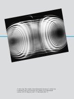
Consider the flow of air around a bicyclist moving through still air with velocity V0, as is
shown in Fig. E3.2. Determine the difference in the pressure between points 112 and 122.
V2 = 0
(2)

V1 = V0
(1)

■ FIGURE E3.2

SOLUTION
In a coordinate system fixed to the bike, it appears as though the air is flowing steadily toward the bicyclist with speed V0. If the assumptions of Bernoulli’s equation are valid 1steady,
incompressible, inviscid flow2, Eq. 3.7 can be applied as follows along the streamline that
passes through 112 and 122
p1 ϩ 12 rV 21 ϩ gz1 ϭ p2 ϩ 12 rV 22 ϩ gz2


We consider 112 to be in the free stream so that V1 ϭ V0 and 122 to be at the tip of the bicyclist’s nose and assume that z1 ϭ z2 and V2 ϭ 0 1both of which, as is discussed in Section 3.4,
are reasonable assumptions2. It follows that the pressure at 122 is greater than that at 112 by
an amount
p2 Ϫ p1 ϭ 12 rV 21 ϭ 12 rV 20

(Ans)

A similar result was obtained in Example 3.1 by integrating the pressure gradient, which
was known because the velocity distribution along the streamline, V1s2, was known. The
Bernoulli equation is a general integration of F ϭ ma. To determine p2 Ϫ p1, knowledge of
the detailed velocity distribution is not needed—only the “boundary conditions” at 112 and
122 are required. Of course, knowledge of the value of V along the streamline is needed to
determine the pressure at points between 112 and 122. Note that if we measure p2 Ϫ p1 we can
determine the speed, V0. As discussed in Section 3.5, this is the principle upon which many
velocity measuring devices are based.
If the bicyclist were accelerating or decelerating, the flow would be unsteady 1i.e., V0
constant2 and the above analysis would be incorrect since Eq. 3.7 is restricted to steady flow.

The difference in fluid velocity between two point in a flow field, V1 and V2, can often
be controlled by appropriate geometric constraints of the fluid. For example, a garden hose
nozzle is designed to give a much higher velocity at the exit of the nozzle than at its entrance
where it is attached to the hose. As is shown by the Bernoulli equation, the pressure within


7708d_c03_109 8/10/01 3:13 PM Page 109 mac120 mac120:1st shift:

3.3 F ϭ ma Normal to a Streamline ■

109


the hose must be larger than that at the exit 1for constant elevation, an increase in velocity
requires a decrease in pressure if Eq. 3.7 is valid2. It is this pressure drop that accelerates the
water through the nozzle. Similarly, an airfoil is designed so that the fluid velocity over its
upper surface is greater 1on the average2 than that along its lower surface. From the Bernoulli
equation, therefore, the average pressure on the lower surface is greater than that on the upper surface. A net upward force, the lift, results.

3.3

F ‫ ؍‬ma Normal to a Streamline
In this section we will consider application of Newton’s second law in a direction normal to
the streamline. In many flows the streamlines are relatively straight, the flow is essentially
one-dimensional, and variations in parameters across streamlines 1in the normal direction2
can often be neglected when compared to the variations along the streamline. However, in
numerous other situations valuable information can be obtained from considering F ϭ ma
normal to the streamlines. For example, the devastating low-pressure region at the center of
a tornado can be explained by applying Newton’s second law across the nearly circular streamlines of the tornado.
We again consider the force balance on the fluid particle shown in Fig. 3.3. This time,
however, we consider components in the normal direction, n
ˆ , and write Newton’s second law
in this direction as
a dFn ϭ

r dV
Ϫ V2
dm V 2
ϭ
r
r


(3.8)

where g dFn represents the sum of n components of all the forces acting on the particle. We
assume the flow is steady with a normal acceleration an ϭ V 2րr, where r is the local radius of curvature of the streamlines. This acceleration is produced by the change in direction of the particle’s velocity as it moves along a curved path.
We again assume that the only forces of importance are pressure and gravity. The component of the weight 1gravity force2 in the normal direction is
dwn ϭ Ϫdw cos u ϭ Ϫg dV
Ϫ cos u
To apply F ‫ ؍‬ma
normal to streamlines, the normal
components of
force are needed.

If the streamline is vertical at the point of interest, u ϭ 90°, and there is no component of
the particle weight normal to the direction of flow to contribute to its acceleration in that
direction.
If the pressure at the center of the particle is p, then its values on the top and bottom
of the particle are p ϩ dpn and p Ϫ dpn, where dpn ϭ 10pր 0n21dn ր22. Thus, if dFpn is the net
pressure force on the particle in the normal direction, it follows that
dFpn ϭ 1 p Ϫ dpn 2 ds dy Ϫ 1 p ϩ dpn 2 ds dy ϭ Ϫ2 dpn ds dy
ϭϪ

0p
0p
ds dn dy ϭ Ϫ dV
Ϫ
0n
0n

Hence, the net force acting in the normal direction on the particle shown in Fig 3.3 is given
by

0p
Ϫ
a dFn ϭ dwn ϩ dFpn ϭ aϪg cos u Ϫ 0n b dV

(3.9)

By combining Eqs. 3.8 and 3.9 and using the fact that along a line normal to the streamline


7708d_c03_110 8/10/01 3:13 PM Page 110 mac120 mac120:1st shift:

110

■ Chapter 3 / Elementary Fluid Dynamics—The Bernoulli Equation

cos u ϭ dzրdn 1see Fig. 3.32, we obtain the following equation of motion along the normal
direction
rV 2
0p
dz
Ϫg
Ϫ
ϭ
(3.10)
dn
0n
r
Weight and/or pressure can produce
curved streamlines.


The physical interpretation of Eq. 3.10 is that a change in the direction of flow of a
fluid particle 1i.e., a curved path, r 6 ϱ 2 is accomplished by the appropriate combination
of pressure gradient and particle weight normal to the streamline. A larger speed or density
or a smaller radius of curvature of the motion requires a larger force unbalance to produce
the motion. For example, if gravity is neglected 1as is commonly done for gas flows2 or if
the flow is in a horizontal 1dzրdn ϭ 02 plane, Eq. 3.10 becomes
rV 2
0p
ϭϪ
0n
r
This indicates that the pressure increases with distance away from the center of curvature
1 0p ր 0n is negative since rV 2 րr is positive—the positive n direction points toward the “inside” of the curved streamline2. Thus, the pressure outside a tornado 1typical atmospheric
pressure2 is larger than it is near the center of the tornado 1where an often dangerously low
partial vacuum may occur2. This pressure difference is needed to balance the centrifugal acceleration associated with the curved streamlines of the fluid motion. (See the photograph at
the beginning of Chapter 2.)

E

XAMPLE
3.3

Shown in Figs. E3.3a, b are two flow fields with circular streamlines. The velocity distributions are
V1r2 ϭ C1r
for case 1a2
and
C2
V1r2 ϭ
for case 1b2
r

where C1 and C2 are constant. Determine the pressure distributions, p ϭ p1r2, for each, given
that p ϭ p0 at r ϭ r0.
p

y

y
V = C1r

(a)

V = C2/r
(b)

r=᏾

x

x

p0

n
(a)

r0

(b)

r

(c)

■ FIGURE E3.3

SOLUTION
We assume the flows are steady, inviscid, and incompressible with streamlines in the horizontal plane 1dzրdn ϭ 02. Since the streamlines are circles, the coordinate n points in a direction opposite to that of the radial coordinate, 0 ր 0n ϭ Ϫ0 ր 0r, and the radius of curvature
is given by r ϭ r. Hence, Eq. 3.10 becomes
rV 2
0p
ϭ
r
0r


7708d_c03_111 8/10/01 3:13 PM Page 111 mac120 mac120:1st shift:

3.4 Physical Interpretation ■

111

For case 1a2 this gives
0p
ϭ rC 21r
0r

while for case 1b2 it gives

V3.2 Free vortex

The sum of pressure, elevation, and

velocity effects is
constant across
streamlines.

rC 22
0p
ϭ 3
0r
r
For either case the pressure increases as r increases since 0p ր 0r 7 0. Integration of these
equations with respect to r, starting with a known pressure p ϭ p0 at r ϭ r0, gives
1
p ϭ rC 21 1r 2 Ϫ r 20 2 ϩ p0
(Ans)
2
for case 1a2 and
1
1
1
p ϭ rC 22 a 2 Ϫ 2 b ϩ p0
(Ans)
2
r0
r
for case 1b2. These pressure distributions are sketched in Fig. E3.3c. The pressure distributions needed to balance the centrifugal accelerations in cases 1a2 and 1b2 are not the same because the velocity distributions are different. In fact for case 1a2 the pressure increases without bound as r S ϱ, while for case 1b2 the pressure approaches a finite value as r S ϱ. The
streamline patterns are the same for each case, however.
Physically, case 1a2 represents rigid body rotation 1as obtained in a can of water on a
turntable after it has been “spun up”2 and case 1b2 represents a free vortex 1an approximation
of a tornado or the swirl of water in a drain, the “bathtub vortex”2. (See the photograph at
the beginning of Chapter 4 for an approximation of this type of flow.)


If we multiply Eq. 3.10 by dn, use the fact that 0pր 0n ϭ dp րdn if s is constant, and integrate
across the streamline 1in the n direction2 we obtain

Ύ

dp
ϩ
r

V2

Ύ r dn ϩ gz ϭ constant across the streamline

(3.11)

To complete the indicated integrations, we must know how the density varies with pressure and how the fluid speed and radius of curvature vary with n. For incompressible flow
the density is constant and the integration involving the pressure term gives simply pրr. We
are still left, however, with the integration of the second term in Eq. 3.11. Without knowing
the n dependence in V ϭ V1s, n2 and r ϭ r1s, n2 this integration cannot be completed.
Thus, the final form of Newton’s second law applied across the streamlines for steady,
inviscid, incompressible flow is
pϩr

Ύ

V2
dn ϩ yz ϭ constant across the streamline
r


(3.12)

As with the Bernoulli equation, we must be careful that the assumptions involved in the derivation of this equation are not violated when it is used.

3.4

Physical Interpretation
In the previous two sections, we developed the basic equations governing fluid motion under a fairly stringent set of restrictions. In spite of the numerous assumptions imposed on
these flows, a variety of flows can be readily analyzed with them. A physical interpretation


7708d_c03_112 8/10/01 3:14 PM Page 112 mac120 mac120:1st shift:

112

■ Chapter 3 / Elementary Fluid Dynamics—The Bernoulli Equation

of the equations will be of help in understanding the processes involved. To this end, we
rewrite Eqs. 3.7 and 3.12 here and interpret them physically. Application of F ϭ ma along
and normal to the streamline results in
p ϩ 12 rV 2 ϩ gz ϭ constant along the streamline

(3.13)

and
pϩr

Ύ

V2

dn ϩ gz ϭ constant across the streamline
r

(3.14)

The following basic assumptions were made to obtain these equations: The flow is steady
and the fluid is inviscid and incompressible. In practice none of these assumptions is exactly
true.
A violation of one or more of the above assumptions is a common cause for obtaining
an incorrect match between the “real world” and solutions obtained by use of the Bernoulli
equation. Fortunately, many “real-world” situations are adequately modeled by the use of
Eqs. 3.13 and 3.14 because the flow is nearly steady and incompressible and the fluid behaves as if it were nearly inviscid.
The Bernoulli equation was obtained by integration of the equation of motion along
the “natural” coordinate direction of the streamline. To produce an acceleration, there must
be an unbalance of the resultant forces, of which only pressure and gravity were considered
to be important. Thus, there are three processes involved in the flow—mass times acceleration 1the rV 2 ր2 term2, pressure 1the p term2, and weight 1the gz term2.
Integration of the equation of motion to give Eq. 3.13 actually corresponds to the workenergy principle often used in the study of dynamics [see any standard dynamics text 1Ref. 12].
This principle results from a general integration of the equations of motion for an object in
a way very similar to that done for the fluid particle in Section 3.2. With certain assumptions, a statement of the work-energy principle may be written as follows:
The work done on a particle by all forces acting on the particle is equal to the change
of the kinetic energy of the particle.

The Bernoulli
equation can be
written in terms of
heights called
heads.

The Bernoulli equation is a mathematical statement of this principle.
As the fluid particle moves, both gravity and pressure forces do work on the particle.

Recall that the work done by a force is equal to the product of the distance the particle travels times the component of force in the direction of travel 1i.e., work ϭ F ؒ d2. The terms gz
and p in Eq. 3.13 are related to the work done by the weight and pressure forces, respectively. The remaining term, rV 2 ր2, is obviously related to the kinetic energy of the particle.
In fact, an alternate method of deriving the Bernoulli equation is to use the first and second
laws of thermodynamics 1the energy and entropy equations2, rather than Newton’s second
law. With the appropriate restrictions, the general energy equation reduces to the Bernoulli
equation. This approach is discussed in Section 5.4.
An alternate but equivalent form of the Bernoulli equation is obtained by dividing each
term of Eq. 3.7 by the specific weight, g, to obtain
p
V2
ϩ z ϭ constant on a streamline
ϩ
g
2g
Each of the terms in this equation has the units of energy per weight 1LFրF ϭ L2 or length
1feet, meters2 and represents a certain type of head.
The elevation term, z, is related to the potential energy of the particle and is called the
elevation head. The pressure term, p րg, is called the pressure head and represents the height
of a column of the fluid that is needed to produce the pressure p. The velocity term, V 2 ր2g,


7708d_c03_113 8/10/01 3:14 PM Page 113 mac120 mac120:1st shift:

3.4 Physical Interpretation ■

113

is the velocity head and represents the vertical distance needed for the fluid to fall freely
1neglecting friction2 if it is to reach velocity V from rest. The Bernoulli equation states that
the sum of the pressure head, the velocity head, and the elevation head is constant along a

streamline.

E

XAMPLE
3.4

Consider the flow of water from the syringe shown in Fig. E3.4. A force applied to the plunger
will produce a pressure greater than atmospheric at point 112 within the syringe. The water
flows from the needle, point 122, with relatively high velocity and coasts up to point 132 at the
top of its trajectory. Discuss the energy of the fluid at points 112, 122, and 132 by using the
Bernoulli equation.
(3)

Energy Type
g

Point
1
2
3

(2)
(1)

F

Kinetic
RV 2ր2


Potential
Gz

Pressure
p

Small
Large
Zero

Zero
Small
Large

Large
Zero
Zero

■ FIGURE E3.4

SOLUTION

If the assumptions 1steady, inviscid, incompressible flow2 of the Bernoulli equation are approximately valid, it then follows that the flow can be explained in terms of the partition of
the total energy of the water. According to Eq. 3.13 the sum of the three types of energy 1kinetic, potential, and pressure2 or heads 1velocity, elevation, and pressure2 must remain constant. The following table indicates the relative magnitude of each of these energies at the
three points shown in the figure.
The motion results in 1or is due to2 a change in the magnitude of each type of energy
as the fluid flows from one location to another. An alternate way to consider this flow is as
follows. The pressure gradient between 112 and 122 produces an acceleration to eject the water from the needle. Gravity acting on the particle between 122 and 132 produces a deceleration to cause the water to come to a momentary stop at the top of its flight.
If friction 1viscous2 effects were important, there would be an energy loss between
112 and 132 and for the given p1 the water would not be able to reach the height indicated in

the figure. Such friction may arise in the needle 1see Chapter 8 on pipe flow2 or between
the water stream and the surrounding air 1see Chapter 9 on external flow2.
A net force is required to accelerate any mass. For steady flow the acceleration can be
interpreted as arising from two distinct occurrences—a change in speed along the streamline and a change in direction if the streamline is not straight. Integration of the equation of
motion along the streamline accounts for the change in speed 1kinetic energy change2 and results in the Bernoulli equation. Integration of the equation of motion normal to the streamline accounts for the centrifugal acceleration 1V 2րr2 and results in Eq. 3.14.


7708d_c03_114 8/10/01 3:14 PM Page 114 mac120 mac120:1st shift:

114

■ Chapter 3 / Elementary Fluid Dynamics—The Bernoulli Equation

The pressure variation across straight
streamlines is hydrostatic.

When a fluid particle travels along a curved path, a net force directed toward the center of curvature is required. Under the assumptions valid for Eq. 3.14, this force may be either
gravity or pressure, or a combination of both. In many instances the streamlines are nearly
straight 1r ϭ ϱ2 so that centrifugal effects are negligible and the pressure variation across
the streamlines is merely hydrostatic 1because of gravity alone2, even though the fluid is in
motion.

E XAMPLE
3.5

Consider the inviscid, incompressible, steady flow shown in Fig. E3.5. From section A to B
the streamlines are straight, while from C to D they follow circular paths. Describe the pressure variation between points 112 and 122 and points 132 and 142.
z

(4)

Free surface
(p = 0)

g

(3) h4-3

(2)

^

n

h2-1

C

(1)

A

D
᏾

■ FIGURE E3.5

B

SOLUTION
With the above assumptions and the fact that r ϭ ϱ for the portion from A to B, Eq. 3.14

becomes
p ϩ gz ϭ constant
The constant can be determined by evaluating the known variables at the two locations using p2 ϭ 0 1gage2, z1 ϭ 0, and z2 ϭ h2–1 to give
p1 ϭ p2 ϩ g1z2 Ϫ z1 2 ϭ p2 ϩ gh2–1

(Ans)

Note that since the radius of curvature of the streamline is infinite, the pressure variation in
the vertical direction is the same as if the fluid were stationary.
However, if we apply Eq. 3.14 between points 132 and 142 we obtain 1using dn ϭ Ϫdz2
p4 ϩ r

Ύ

z4

z3

V2
1Ϫdz2 ϩ gz4 ϭ p3 ϩ gz3
r

With p4 ϭ 0 and z4 Ϫ z3 ϭ h4–3 this becomes
p3 ϭ gh4–3 Ϫ r

Ύ

z4

z3


V2
dz
r

(Ans)

To evaluate the integral, we must know the variation of V and r with z. Even without this
detailed information we note that the integral has a positive value. Thus, the pressure at 132 is
less than the hydrostatic value, gh4–3, by an amount equal to r ͐zz34 1V 2րr2 dz. This lower
pressure, caused by the curved streamline, is necessary to accelerate the fluid around the
curved path.
Note that we did not apply the Bernoulli equation 1Eq. 3.132 across the streamlines
from 112 to 122 or 132 to 142. Rather we used Eq. 3.14. As is discussed in Section 3.8, application of the Bernoulli equation across streamlines 1rather than along them2 may lead to serious errors.


7708d_c03_115 8/10/01 3:15 PM Page 115 mac120 mac120:1st shift:

3.5 Static, Stagnation, Dynamic, and Total Pressure ■

3.5

115

Static, Stagnation, Dynamic, and Total Pressure

Each term in the
Bernoulli equation
can be interpreted
as a form of pressure.


A useful concept associated with the Bernoulli equation deals with the stagnation and dynamic pressures. These pressures arise from the conversion of kinetic energy in a flowing
fluid into a “pressure rise” as the fluid is brought to rest 1as in Example 3.22. In this section
we explore various results of this process. Each term of the Bernoulli equation, Eq. 3.13, has
the dimensions of force per unit area—psi, lb րft2, Nրm2. The first term, p, is the actual thermodynamic pressure of the fluid as it flows. To measure its value, one could move along
with the fluid, thus being “static” relative to the moving fluid. Hence, it is normally termed
the static pressure. Another way to measure the static pressure would be to drill a hole in a
flat surface and fasten a piezometer tube as indicated by the location of point 132 in Fig. 3.4.
As we saw in Example 3.5, the pressure in the flowing fluid at 112 is p1 ϭ gh3–1 ϩ p3, the
same as if the fluid were static. From the manometer considerations of Chapter 2, we know
that p3 ϭ gh4–3. Thus, since h3–1 ϩ h4–3 ϭ h it follows that p1 ϭ gh.

Open

H

(4)

h

h4-3

V
h3-1

(3)

ρ

(1)


(2)

V1 = V

V2 = 0

■ FIGURE 3.4

Measurement
of static and stagnation pressures.

The third term in Eq. 3.13, gz, is termed the hydrostatic pressure, in obvious regard to
the hydrostatic pressure variation discussed in Chapter 2. It is not actually a pressure but
does represent the change in pressure possible due to potential energy variations of the fluid
as a result of elevation changes.
The second term in the Bernoulli equation, rV 2 ր2, is termed the dynamic pressure. Its
interpretation can be seen in Fig. 3.4 by considering the pressure at the end of a small tube
inserted into the flow and pointing upstream. After the initial transient motion has died out,
the liquid will fill the tube to a height of H as shown. The fluid in the tube, including that
at its tip, 122, will be stationary. That is, V2 ϭ 0, or point 122 is a stagnation point.
If we apply the Bernoulli equation between points 112 and 122, using V2 ϭ 0 and assuming that z1 ϭ z2, we find that
p2 ϭ p1 ϩ 12 rV 21

V3.3 Stagnation
point flow

Hence, the pressure at the stagnation point is greater than the static pressure, p1, by an amount
rV 21ր2, the dynamic pressure.
It can be shown that there is a stagnation point on any stationary body that is placed

into a flowing fluid. Some of the fluid flows “over” and some “under” the object. The dividing line 1or surface for two-dimensional flows2 is termed the stagnation streamline and
terminates at the stagnation point on the body. 1See the photograph at the beginning of Chapter 3.2 For symmetrical objects 1such as a sphere2 the stagnation point is clearly at the tip or
front of the object as shown in Fig. 3.5a. For nonsymmetrical objects such as the airplane
shown in Fig. 3.5b, the location of the stagnation point is not always obvious.


7708d_c03_116

116

8/13/01

6:40 PM

Page 116

■ Chapter 3 / Elementary Fluid Dynamics—The Bernoulli Equation
Stagnation point

Stagnation streamline

■ FIGURE 3.5

Stagnation point
( a)

Stagnation points on
bodies in flowing fluids.

( b)


If elevation effects are neglected, the stagnation pressure, p ϩ rV 2 ր2, is the largest
pressure obtainable along a given streamline. It represents the conversion of all of the kinetic
energy into a pressure rise. The sum of the static pressure, hydrostatic pressure, and dynamic
pressure is termed the total pressure, pT. The Bernoulli equation is a statement that the total
pressure remains constant along a streamline. That is,
p ϩ 12 rV 2 ϩ gz ϭ pT ϭ constant along a streamline

V3.4 Airspeed
indicator

(3.15)

Again, we must be careful that the assumptions used in the derivation of this equation are
appropriate for the flow being considered.
Knowledge of the values of the static and stagnation pressures in a fluid implies that the
fluid speed can be calculated. This is the principle on which the Pitot-static tube is based
[H. de Pitot (1675–1771)]. As shown in Fig. 3.6, two concentric tubes are attached to
two pressure gages 1or a differential gage2 so that the values of p3 and p4 1or the difference
p3 Ϫ p42 can be determined. The center tube measures the stagnation pressure at its open tip.
If elevation changes are negligible,
p3 ϭ p ϩ 12 rV 2

where p and V are the pressure and velocity of the fluid upstream of point 122. The outer tube
is made with several small holes at an appropriate distance from the tip so that they measure
the static pressure. If the elevation difference between 112 and 142 is negligible, then
p4 ϭ p1 ϭ p

Pitot-static tubes
measure fluid velocity by converting

velocity into pressure.

By combining these two equations we see that
p3 Ϫ p4 ϭ 12 rV 2
which can be rearranged to give
V ϭ 221 p3 Ϫ p4 2 րr

(3.16)

The actual shape and size of Pitot-static tubes vary considerably. Some of the more common
types are shown in Fig. 3.7.
(3)

(4)

(1)

V
p

(2)

■ FIGURE 3.6

The Pitot-static tube.


7708d_c03_117 8/10/01 3:25 PM Page 117 mac120 mac120:1st shift:

3.5 Static, Stagnation, Dynamic, and Total Pressure ■


117

American Blower company

V

National Physical laboratory (England)

American Society of Heating & Ventilating Engineers

■ FIGURE 3.7

Typical
Pitot-static tube designs.

E XAMPLE
3.6

An airplane flies 100 mi͞hr at an elevation of 10,000 ft in a standard atmosphere as shown
in Fig. E3.6. Determine the pressure at point 112 far ahead of the airplane, the pressure at the
stagnation point on the nose of the airplane, point 122, and the pressure difference indicated
by a Pitot-static probe attached to the fuselage.

V1 = 100 mi/hr

(2)

(1)


■ FIGURE E3.6

Pitot-static tube

SOLUTION
From Table C.1 we find that the static pressure at the altitude given is
p1 ϭ 1456 lbրft2 1abs2 ϭ 10.11 psia

(Ans)

Also, the density is r ϭ 0.001756 slugրft .
If the flow is steady, inviscid, and incompressible and elevation changes are neglected,
Eq. 3.13 becomes
3

p2 ϭ p1 ϩ

rV 21
2

With V1 ϭ 100 miրhr ϭ 146.7 ftրs and V2 ϭ 0 1since the coordinate system is fixed to the
airplane2 we obtain
p2 ϭ 1456 lbրft2 ϩ 10.001756 slugsրft3 21146.72 ft2րs2 2 ր2
ϭ 11456 ϩ 18.92 lbրft2 1abs2

Hence, in terms of gage pressure
p2 ϭ 18.9 lbրft2 ϭ 0.1313 psi

(Ans)


Thus, the pressure difference indicated by the Pitot-static tube is
p2 Ϫ p1 ϭ

rV 21
ϭ 0.1313 psi
2

(Ans)

Note that it is very easy to obtain incorrect results by using improper units. Do not add lbրin.2
and lb րft2. Recall that 1slug րft3 21ft2 րs2 2 ϭ 1slug # ftրs2 2 ր 1ft2 2 ϭ lb րft2.


7708d_c03_118 8/10/01 3:26 PM Page 118 mac120 mac120:1st shift:

118

■ Chapter 3 / Elementary Fluid Dynamics—The Bernoulli Equation

It was assumed that the flow is incompressible—the density remains constant from
112 to 122. However, since r ϭ p րRT, a change in pressure 1or temperature2 will cause a change
in density. For this relatively low speed, the ratio of the absolute pressures is nearly unity
3i.e., p1 րp2 ϭ 110.11 psia2 ր 110.11 ϩ 0.1313 psia2 ϭ 0.9874, so that the density change is
negligible. However, at high speed it is necessary to use compressible flow concepts to obtain accurate results. 1See Section 3.8.1 and Chapter 11.2

V
p

V
p


V
p

■ FIGURE 3.8
(1)
p1 > p

(1)
p1 < p

Incorrect
and correct design of static pressure taps.

(1)
p1 = p

Also, the pressure along the surface of an object varies from the stagnation pressure at
its stagnation point to values that may be less than the free stream static pressure. A typical
pressure variation for a Pitot-static tube is indicated in Fig. 3.9. Clearly it is important that
the pressure taps be properly located to ensure that the pressure measured is actually the static pressure.
In practice it is often difficult to align the Pitot-static tube directly into the flow direction. Any misalignment will produce a nonsymmetrical flow field that may introduce errors. Typically, yaw angles up to 12 to 20° 1depending on the particular probe design2 give
results that are less than 1% in error from the perfectly aligned results. Generally it is more
difficult to measure static pressure than stagnation pressure.
One method of determining the flow direction and its speed 1thus the velocity2 is to use
a directional-finding Pitot tube as is illustrated in Fig. 3.10. Three pressure taps are drilled
into a small circular cylinder, fitted with small tubes, and connected to three pressure transducers. The cylinder is rotated until the pressures in the two side holes are equal, thus indicating that the center hole points directly upstream. The center tap then measures the stagp
V

(2)

(1)

Stagnation
pressure at
tip

Tube
Stagnation
pressure on
stem

(1)
0

(2)

Static
pressure

Stem

Accurate measurement of static pressure requires great
care.

The Pitot-static tube provides a simple, relatively inexpensive way to measure fluid
speed. Its use depends on the ability to measure the static and stagnation pressures. Care is
needed to obtain these values accurately. For example, an accurate measurement of static
pressure requires that none of the fluid’s kinetic energy be converted into a pressure rise at
the point of measurement. This requires a smooth hole with no burrs or imperfections. As
indicated in Fig. 3.8, such imperfections can cause the measured pressure to be greater or

less than the actual static pressure.

■ FIGURE 3.9

Typical
pressure distribution along a
Pitot-static tube.


7708d_c03_119 8/10/01 3:26 PM Page 119 mac120 mac120:1st shift:

3.6 Examples of Use of the Bernoulli Equation ■

(3)

β

If θ = 0

p1 = p3 = p

(2)

θ

V
p

Many velocity measuring devices use
Pitot-static tube

principles.

3.6

β

119

_ ρ V2
p2 = p + 1

(1)

2

■ F I G U R E 3 . 1 0 Cross section of a directional-finding Pitotstatic tube.

nation pressure. The two side holes are located at a specific angle 1b ϭ 29.5°2 so that they
measure the static pressure. The speed is then obtained from V ϭ 321 p2 Ϫ p1 2 րr4 1ր2.
The above discussion is valid for incompressible flows. At high speeds, compressibility becomes important 1the density is not constant2 and other phenomena occur. Some of these
ideas are discussed in Section 3.8, while others 1such as shockwaves for supersonic Pitottube applications2 are discussed in Chapter 11.
The concepts of static, dynamic, stagnation, and total pressure are useful in a variety
of flow problems. These ideas are used more fully in the remainder of the book.

Examples of Use of the Bernoulli Equation
In this section we illustrate various additional applications of the Bernoulli equation. Between any two points, 112 and 122, on a streamline in steady, inviscid, incompressible flow the
Bernoulli equation can be applied in the form
p1 ϩ 12 rV 21 ϩ gz1 ϭ p2 ϩ 12 rV 22 ϩ gz2

(3.17)


Obviously if five of the six variables are known, the remaining one can be determined. In
many instances it is necessary to introduce other equations, such as the conservation of mass.
Such considerations will be discussed briefly in this section and in more detail in Chapter 5.

3.6.1

Free Jets

One of the oldest equations in fluid mechanics deals with the flow of a liquid from a large
reservoir, as is shown in Fig. 3.11. A jet of liquid of diameter d flows from the nozzle with
velocity V as shown. 1A nozzle is a device shaped to accelerate a fluid.2 Application of Eq. 3.17
between points 112 and 122 on the streamline shown gives
gh ϭ 12 rV 2

(1)

h

z
(3)

ᐉ

V3.5 Flow from a
tank

(2)

(2)


d
H

V
(5)

(4)

■ FIGURE 3.11

Vertical flow from a tank.


7708d_c03_120

120

8/13/01

1:35 AM

Page 120

■ Chapter 3 / Elementary Fluid Dynamics—The Bernoulli Equation

We have used the facts that z1 ϭ h, z2 ϭ 0, the reservoir is large 1V1 Х 02, open to the atmosphere 1 p1 ϭ 0 gage2, and the fluid leaves as a “free jet” 1 p2 ϭ 02. Thus, we obtain
Vϭ

The exit pressure

for an incompressible fluid jet is
equal to the surrounding pressure.

B

2

gh
ϭ 12gh
r

(3.18)

which is the modern version of a result obtained in 1643 by Torricelli 11608–16472, an Italian physicist.
The fact that the exit pressure equals the surrounding pressure 1 p2 ϭ 02 can be seen
by applying F ϭ ma, as given by Eq. 3.14, across the streamlines between 122 and 142. If the
streamlines at the tip of the nozzle are straight 1r ϭ ϱ2, it follows that p2 ϭ p4. Since 142 is
on the surface of the jet, in contact with the atmosphere, we have p4 ϭ 0. Thus, p2 ϭ 0 also.
Since 122 is an arbitrary point in the exit plane of the nozzle, it follows that the pressure is
atmospheric across this plane. Physically, since there is no component of the weight force or
acceleration in the normal 1horizontal2 direction, the pressure is constant in that direction.
Once outside the nozzle, the stream continues to fall as a free jet with zero pressure
throughout 1 p5 ϭ 02 and as seen by applying Eq. 3.17 between points 112 and 152, the speed
increases according to
V ϭ 12g 1h ϩ H2

where H is the distance the fluid has fallen outside the nozzle.
Equation 3.18 could also be obtained by writing the Bernoulli equation between points
132 and 142 using the fact that z4 ϭ 0, z3 ϭ /. Also, V3 ϭ 0 since it is far from the nozzle, and
from hydrostatics, p3 ϭ g1h Ϫ /2.

Recall from physics or dynamics that any object dropped from rest through a distance
h in a vacuum will obtain the speed V ϭ 12gh, the same as the liquid leaving the nozzle.
This is consistent with the fact that all of the particle’s potential energy is converted to kinetic energy, provided viscous 1friction2 effects are negligible. In terms of heads, the elevation head at point 112 is converted into the velocity head at point 122. Recall that for the case
shown in Fig. 3.11 the pressure is the same 1atmospheric2 at points 112 and 122.
For the horizontal nozzle of Fig. 3.12, the velocity of the fluid at the centerline, V2,
will be slightly greater than that at the top, V1, and slightly less than that at the bottom, V3,
due to the differences in elevation. In general, d Ӷ h and we can safely use the centerline
velocity as a reasonable “average velocity.”
If the exit is not a smooth, well-contoured nozzle, but rather a flat plate as shown in
Fig. 3.13, the diameter of the jet, dj, will be less than the diameter of the hole, dh. This phenomenon, called a vena contracta effect, is a result of the inability of the fluid to turn the
sharp 90° corner indicated by the dotted lines in the figure.

(1)

h
d

dh

dj
a

(2)

(1)

(3)

a


(2)
(3)

■ FIGURE 3.12

tal flow from a tank.

■ FIGURE 3.13

Horizon-

Vena
contracta effect for a sharp-edged
orifice.


7708d_c03_121 8/10/01 3:26 PM Page 121 mac120 mac120:1st shift:

3.6 Examples of Use of the Bernoulli Equation ■

The diameter of a
fluid jet is often
smaller than that of
the hole from
which it flows.

121

Since the streamlines in the exit plane are curved 1r 6 ϱ2, the pressure across them
is not constant. It would take an infinite pressure gradient across the streamlines to cause the

fluid to turn a “sharp” corner 1r ϭ 02. The highest pressure occurs along the centerline at
122 and the lowest pressure, p1 ϭ p3 ϭ 0, is at the edge of the jet. Thus, the assumption of
uniform velocity with straight streamlines and constant pressure is not valid at the exit plane.
It is valid, however, in the plane of the vena contracta, section a–a. The uniform velocity assumption is valid at this section provided dj Ӷ h, as is discussed for the flow from the nozzle
shown in Fig. 3.12.
The vena contracta effect is a function of the geometry of the outlet. Some typical configurations are shown in Fig. 3.14 along with typical values of the experimentally obtained
contraction coefficient, Cc ϭ AjրAh, where Aj and Ah are the areas of the jet at the vena contracta and the area of the hole, respectively.

dj

dh

CC = 0.61

CC = 1.0

CC = A j /A h = (dj /dh)2

CC = 0.50
CC = 0.61

■ F I G U R E 3 . 1 4 Typical flow patterns and contraction coefficients for various round exit configurations.

3.6.2

Confined Flows

In many cases the fluid is physically constrained within a device so that its pressure cannot
be prescribed a priori as was done for the free jet examples above. Such cases include nozzles
and pipes of variable diameter for which the fluid velocity changes because the flow area is

different from one section to another. For these situations it is necessary to use the concept
of conservation of mass 1the continuity equation2 along with the Bernoulli equation. The derivation and use of this equation are discussed in detail in Chapters 4 and 5. For the needs
of this chapter we can use a simplified form of the continuity equation obtained from the
following intuitive arguments. Consider a fluid flowing through a fixed volume 1such as a
tank2 that has one inlet and one outlet as shown in Fig. 3.15. If the flow is steady so that
there is no additional accumulation of fluid within the volume, the rate at which the fluid
flows into the volume must equal the rate at which it flows out of the volume 1otherwise,
mass would not be conserved2.


7708d_c03_122 8/10/01 3:27 PM Page 122 mac120 mac120:1st shift:

122

■ Chapter 3 / Elementary Fluid Dynamics—The Bernoulli Equation

V1 δ t

Fluid parcel at t = 0
Same parcel at t = δ t

V1

(1)
Volume = V1 δ t A1

V2 δ t

V2


■ FIGURE 3.15

The continuity
equation states that
mass cannot be created or destroyed.

Volume = V2 δ t A2

(2)

Steady flow into and out of a tank.

#
#
The mass flowrate from an outlet, m 1slugs͞s or kg͞s2, is given by m ϭ rQ, where Q
1ft3րs or m3րs2 is the volume flowrate. If the outlet area is A and the fluid flows across this
area 1normal to the area2 with an average velocity V, then the volume of the fluid crossing
this area in a time interval dt is VA dt, equal to that in a volume of length V dt and crosssectional area A 1see Fig. 3.152. Hence, the volume flowrate 1volume per unit time2 is Q ϭ VA.
#
Thus, m ϭ rVA. To conserve mass, the inflow rate must equal the outflow rate. If the inlet
#
#
is designated as 112 and the outlet as 122, it follows that m1 ϭ m2. Thus, conservation of mass
requires
r1A1V1 ϭ r2A2V2
If the density remains constant, then r1 ϭ r2, and the above becomes the continuity equation for incompressible flow
A1V1 ϭ A2V2, or Q1 ϭ Q2

(3.19)


For example, if the outlet flow area is one-half the size of the inlet flow area, it follows that
the outlet velocity is twice that of the inlet velocity, since V2 ϭ A1V1 րA2 ϭ 2V1. (See the photograph at the beginning of Chapter 5.) The use of the Bernoulli equation and the flowrate
equation 1continuity equation2 is demonstrated by Example 3.7.

E

XAMPLE
3.7

A stream of water of diameter d ϭ 0.1 m flows steadily from a tank of diameter D ϭ 1.0 m
as shown in Fig. E3.7a. Determine the flowrate, Q, needed from the inflow pipe if the water depth remains constant, h ϭ 2.0 m.
Q

1.10

(1)

Q/Q0 1.05

D = 1.0 m
h = 2.0 m

(2)
1.00

0

d = 0.10 m
(a)


0.2

0.4

0.6

0.8

d/D
(b )

■ FIGURE E3.7

SOLUTION

For steady, inviscid, incompressible flow, the Bernoulli equation applied between points 112
and 122 is


7708d_c03_123 8/10/01 3:27 PM Page 123 mac120 mac120:1st shift:

3.6 Examples of Use of the Bernoulli Equation ■

p1 ϩ 12 rV 21 ϩ gz1 ϭ p2 ϩ 12 rV 22 ϩ gz2

123
(1)

With the assumptions that p1 ϭ p2 ϭ 0, z1 ϭ h, and z2 ϭ 0, Eq. 1 becomes
1 2

2V 1

ϩ gh ϭ 12 V 22

(2)

Although the water level remains constant 1h ϭ constant2, there is an average velocity, V1,
across section 112 because of the flow from the tank. From Eq. 3.19 for steady incompressible flow, conservation of mass requires Q1 ϭ Q2, where Q ϭ AV. Thus, A1V1 ϭ A2V2, or
p 2
p
D V1 ϭ d 2V2
4
4
Hence,
d 2
V1 ϭ a b V2
D

(3)

Equations 1 and 3 can be combined to give
V2 ϭ

219.81 mրs2 212.0 m2
2gh
ϭ
ϭ 6.26 mրs
B 1 Ϫ 1dրD2 4 B 1 Ϫ 10.1mր1m2 4

Thus,

Q ϭ A1V1 ϭ A2V2 ϭ

p
10.1 m2 2 16.26 mրs2 ϭ 0.0492 m3 րs
4

(Ans)

In this example we have not neglected the kinetic energy of the water in the tank
1V1 02. If the tank diameter is large compared to the jet diameter 1D ӷ d2, Eq. 3 indicates
that V1 Ӷ V2 and the assumption that V1 Ϸ 0 would be reasonable. The error associated with
this assumption can be seen by calculating the ratio of the flowrate assuming V1 0, denoted Q, to that assuming V1 ϭ 0, denoted Q0. This ratio, written as
22gh ր 31 Ϫ 1d րD2 4 4
V2
Q
1
ϭ
ϭ
ϭ
Q0
V2 0 Dϭϱ
22gh
21 Ϫ 1d րD2 4

is plotted in Fig. E3.7b. With 0 6 dրD 6 0.4 it follows that 1 6 QրQ0 Շ 1.01, and the error in assuming V1 ϭ 0 is less than 1%. Thus, it is often reasonable to assume V1 ϭ 0.

The fact that a kinetic energy change is often accompanied by a change in pressure is
shown by Example 3.8.

E


XAMPLE
3.8

Air flows steadily from a tank, through a hose of diameter D ϭ 0.03 m and exits to the atmosphere from a nozzle of diameter d ϭ 0.01 m as shown in Fig. E3.8. The pressure in the
tank remains constant at 3.0 kPa 1gage2 and the atmospheric conditions are standard temperature and pressure. Determine the flowrate and the pressure in the hose.
p1 = 3.0 kPa

D = 0.03 m

d = 0.01 m
Q

(2)
(1)

Air

(3)

■ FIGURE E3.8


7708d_c03_124 8/10/01 3:27 PM Page 124 mac120 mac120:1st shift:

124

■ Chapter 3 / Elementary Fluid Dynamics—The Bernoulli Equation

SOLUTION

If the flow is assumed steady, inviscid, and incompressible, we can apply the Bernoulli equation along the streamline shown as
p1 ϩ 12 rV 21 ϩ gz1 ϭ p2 ϩ 12 rV 22 ϩ gz2
ϭ p3 ϩ 12 rV 23 ϩ gz3

With the assumption that z1 ϭ z2 ϭ z3 1horizontal hose2, V1 ϭ 0 1large tank2, and p3 ϭ 0 1free
jet2, this becomes
V3 ϭ

2p1
B r

and
p2 ϭ p1 Ϫ 12 rV 22

(1)

The density of the air in the tank is obtained from the perfect gas law, using standard absolute pressure and temperature, as
rϭ

p1
RT1

ϭ 3 13.0 ϩ 1012 kNրm2 4
ϫ

103 N րkN
1286.9 N᝽mրkg᝽K2115 ϩ 2732K

ϭ 1.26 kgրm3
Thus, we find that

V3 ϭ

B

213.0 ϫ 103 Nրm2 2
1.26 kg րm3

ϭ 69.0 mրs

or
Q ϭ A3 V3 ϭ

p 2
p
d V3 ϭ 10.01 m2 2 169.0 mրs2
4
4

ϭ 0.00542 m3 րs

(Ans)

Note that the value of V3 is determined strictly by the value of p1 1and the assumptions involved in the Bernoulli equation2, independent of the “shape” of the nozzle. The pressure
head within the tank, p1 րg ϭ 13.0 kPa2 ր 19.81 mրs2 211.26 kg րm3 2 ϭ 243 m, is converted to
the velocity head at the exit, V 22ր2g ϭ 169.0 mրs2 2 ր 12 ϫ 9.81 mրs2 2 ϭ 243 m. Although we
used gage pressure in the Bernoulli equation 1 p3 ϭ 02, we had to use absolute pressure in
the perfect gas law when calculating the density.
The pressure within the hose can be obtained from Eq. 1 and the continuity equation
1Eq. 3.192
A2V2 ϭ A3V3

Hence,
d 2
0.01 m 2
b 169.0 mրs2 ϭ 7.67 mրs
V2 ϭ A3V3 րA2 ϭ a b V3 ϭ a
D
0.03 m