Iterative chase decoding of algebraic geometric codes
Bạn đang xem bản rút gọn của tài liệu. Xem và tải ngay bản đầy đủ của tài liệu tại đây (1.09 MB, 79 trang )
ITERATIVE CHASE DECODING OF ALGEBRAIC GEOMETRIC
CODES
HU WENGUANG
NATIONAL UNIVERSITY OF SINGAPORE
2005
ITERATIVE CHASE DECODING OF ALGEBRAIC GEOMETRIC
CODES
HU WENGUANG
(B.Eng.,THU, P.R.CHINA)
A THESIS SUBMITTED
FOR THE DEGREE OF MASTER OF ENGINEERING
DEPARTMENT OF ELECTRICAL AND COMPUTER ENGINEERING
NATIONAL UNIVERSITY OF SINGAPORE
2005
Acknowledgement
I wish to thank Dr. Marc Andre Armand and Dr. Mehul Motani for their
patient and invaluable guidance throughout the courses of my project and thesis.
I am grateful for, and much enlightened from the numerous discussions with them.
I sincerely wish them all the best in all their future endeavors.
I would also like to thank my friend Cai Feng for the fruitful discussions which
helped me to solve the some problems in this thesis. My gratitude also goes to National University of Singapore who provides me an excellent research environment
and grants me the use of the facilities and scholarship.
I am also grateful to my wife,my parents and my elder brother, who always
support and encourage me, without which even the easiest thing would not have
been possible for me.
i
Contents
Abbreviations
v
List of Figures
vi
List of Tables
vi
Summary
viii
1 Introduction
1.1
1
Error Control Coding . . . . . . . . . . . . . . . . . . . . . . . . . .
1
1.1.1
Reed-Solomon Codes . . . . . . . . . . . . . . . . . . . . . .
4
1.1.2
Algebraic Geometric Codes . . . . . . . . . . . . . . . . . .
5
Hard-decision and Soft-decision Decoding . . . . . . . . . . . . . . .
6
1.2.1
Chase Decoding . . . . . . . . . . . . . . . . . . . . . . . . .
6
1.2.2
Turbo Codes and Iterative Decoding . . . . . . . . . . . . .
7
1.3
Contributions of this Thesis . . . . . . . . . . . . . . . . . . . . . .
8
1.4
Thesis Outline . . . . . . . . . . . . . . . . . . . . . . . . . . . . . .
8
1.2
2 Algebraic Geometric Codes
10
2.1
Introduction . . . . . . . . . . . . . . . . . . . . . . . . . . . . . . .
10
2.2
Definition of Algebraic-Geometric Codes . . . . . . . . . . . . . . .
11
2.2.1
Algebraic Function Fields and Algebraic Curves . . . . . . .
ii
12
2.2.2
2.3
Divisors and Vector Space . . . . . . . . . . . . . . . . . . .
14
Hermitian Codes . . . . . . . . . . . . . . . . . . . . . . . . . . . .
17
2.3.1
Basis of the Hermitian Function Field . . . . . . . . . . . .
17
2.3.2
Generator Matrix of Hermitian Codes . . . . . . . . . . . . .
19
2.3.3
The relationship between Hermitian Codes and Generalized
Reed-Solomon Codes . . . . . . . . . . . . . . . . . . . . . .
20
Residual Algebraic Geometric Codes over Klein Quartic Curves . .
22
2.4.1
Rational Points of Klein Quartic Curve . . . . . . . . . . . .
23
2.4.2
Codes Definition and Parameters . . . . . . . . . . . . . . .
23
2.4.3
Function Field Basis for Klein Quartic Curve . . . . . . . . .
25
2.4.4
Parity Check Matrix and Generator Matrix . . . . . . . . .
26
2.5
Asymptotically Good AG Codes . . . . . . . . . . . . . . . . . . . .
27
2.6
Summary . . . . . . . . . . . . . . . . . . . . . . . . . . . . . . . .
31
2.4
3 Chase Decoding of AG Codes
33
3.1
Introduction . . . . . . . . . . . . . . . . . . . . . . . . . . . . . . .
33
3.2
Parallel Berlekamp-Massey Algorithm . . . . . . . . . . . . . . . . .
34
3.3
Soft-Decision Decoding . . . . . . . . . . . . . . . . . . . . . . . . .
34
3.4
The Chase Algorithm . . . . . . . . . . . . . . . . . . . . . . . . . .
35
3.4.1
General Description . . . . . . . . . . . . . . . . . . . . . . .
35
3.4.2
The Chase Algorithm in Fading Channels . . . . . . . . . .
38
3.4.3
The Chase Algorithm for Non-Binary Block Codes . . . . .
39
3.5
Simulation Results and Discussion . . . . . . . . . . . . . . . . . . .
41
3.6
Summary . . . . . . . . . . . . . . . . . . . . . . . . . . . . . . . .
45
4 Block Turbo Codes
4.1
46
Introduction . . . . . . . . . . . . . . . . . . . . . . . . . . . . . . .
iii
46
4.2
Product Codes . . . . . . . . . . . . . . . . . . . . . . . . . . . . .
47
4.3
Iterative Chase Decoding of Product Codes . . . . . . . . . . . . . .
50
4.3.1
Reliability of a Decision Given by Soft-Input Decoder . . . .
52
4.3.2
Codeword Validation . . . . . . . . . . . . . . . . . . . . . .
53
4.3.3
Parameter Settings . . . . . . . . . . . . . . . . . . . . . . .
54
4.4
Simulation Results and Discussions . . . . . . . . . . . . . . . . . .
55
4.5
Summary . . . . . . . . . . . . . . . . . . . . . . . . . . . . . . . .
62
5 Conclusion
63
5.1
Summary of Thesis . . . . . . . . . . . . . . . . . . . . . . . . . . .
63
5.2
Future Work . . . . . . . . . . . . . . . . . . . . . . . . . . . . . . .
64
Bibliography
66
iv
Abbreviations
AG Code: Algebraic Geometric Code
AWGN Channel: Additive White Gaussian Noise Channel
BCH Code: Bose-Chaudhuri-Hocquenghem Code
BER: Bit Error Rate
BPSK: Binary Phase Shift Keying
BTC: Block Turbo Code
CTC: Convolutional Turbo Code
LLR: Log-Likelihood-Ratio
MAP: Maximum a-Posteriori Probability
MDS Codes: Maximum Distance Separable Codes
MLD: Maximum Likelihood Decoding
OSD: Ordered Statistics Decoding
PBMA: Parallel implementation of Berlekamp-Massey Algorithm
SISO: Soft-Input Soft-Output
SNR: Signal-to-Noise Ratio
RS Code: Reed-Solomon Code
v
List of Figures
1.1
Block diagram of a digital communication system . . . . . . . . . .
2
3.1
Flow Chart of Chase Algorithm . . . . . . . . . . . . . . . . . . . .
38
3.2
Performace of Chase Decoding of (23,18,3) AG codes over Klein
quartic curves in AWGN channel . . . . . . . . . . . . . . . . . . .
3.3
42
Performace of Chase Decoding of (23,18,3) AG codes over Klein
quartic curves in Rayleigh fading channel . . . . . . . . . . . . . . .
44
4.1
Product Codes . . . . . . . . . . . . . . . . . . . . . . . . . . . . .
48
4.2
Non-binary Product Codes with Symbol Concatenation . . . . . . .
50
4.3
Non-binary Product Codes with Bit Concatenation . . . . . . . . .
51
4.4
The Flowchart of Iterative Chase Decoding . . . . . . . . . . . . . .
53
4.5
Performance of Iterative Chase Decoding of (23,18,3) AG codes over
Klein quartic curves in AWGN channel using bit concatenation . . .
4.6
Performance of Iterative Chase Decoding of (23,18,3) AG codes over
Klein quartic curves in AWGN channel using symbol concatenation
4.7
58
Performance of Iterative Chase Decoding of (23,18,3) AG codes over
Klein quartic curves in Rayleigh channel using bit concatenation . .
4.8
57
59
Performance of Iterative Chase Decoding of (23,18,3) AG codes over
Klein quartic curves in Rayleigh channel using symbol concatenation 61
vi
List of Tables
2.1
Rational Points of Hermitian Curve . . . . . . . . . . . . . . . . . .
22
2.2
Rational Points of Klein Quartic Curve over F8 . . . . . . . . . . .
24
2.3
Standard Basis of L(7P∞ ) . . . . . . . . . . . . . . . . . . . . . . .
26
2.4
Parity Check Matrix of (23,18,3) Residual Code over Klein Quartic
Curve . . . . . . . . . . . . . . . . . . . . . . . . . . . . . . . . . .
28
2.5
Generator Matrix of (23,18,3) Residual Code over Klein Quartic Curve 29
3.1
Binary Representation of elements of F8 . . . . . . . . . . . . . . .
4.1
Performance Comparison of BCH product codes and AG product
40
codes . . . . . . . . . . . . . . . . . . . . . . . . . . . . . . . . . . .
60
4.2
Code Parameter of One-point AG Codes over F8 . . . . . . . . . . .
60
4.3
Code Parameter of BCH codes . . . . . . . . . . . . . . . . . . . . .
62
vii
Summary
Error control coding is designed to solve the problem of reliable transmission
of information over a noisy channel. BCH codes and Reed-Solomon codes are two
kinds of widely used error control codes. In the last two decades, various ideas of
algebraic geometry are used in the construction of error control codes and their
decoding algorithms. These codes are usually called algebraic geometric codes.
Algebraic geometric codes could be considered as a generalization of Reed-Solomon
codes. The introduction of turbo codes by Berrou, Glavirux and Thitimajshima
also has considerably modified our approach of channel coding in the last ten
years. Later the general concept of iterative soft-input soft-output decoding has
been extended to block turbo codes(BTC) by Pyndiah. Both BCH codes and ReedSolomon codes have been used in the block turbo decoding scheme. In this thesis,
one-point algebraic geometric codes are used as the component codes of block turbo
codes.
This thesis is intended to investigate the soft-decision decoding algorithms of
algebraic geometric codes to achieve good performance of digital communications
in both AWGN channel and Rayleigh fading channels.
The first part presents the fundamental theory of algebraic geometry, which is
important in the construction of AG codes and their decoding algorithms. Codes
defined over Hermitian curves and Klein quartic curves are selected as the example
of functional AG codes and residual AG codes respectively. Their encoding methods and code parameters are introduced. In addition, the relationship between
functional Hermitian codes and generalized Reed-Solomon codes are shown.
In the second part, we use the Chase algorithm with an inner hard-decision decoder, which is a parallel implementation of Berlekamp-Massey algorithm(PBMA),
viii
in the soft-decision decoding of one-point AG codes over Klein quartic curves. The
simulations in AWGN channel and Rayleigh fading channel shown that the decoding scheme can achieve remarkable coding gains compared with the hard-decision
PBMA decoder.
In the last part, we presented the iterative Chase decoding algorithm for the
product codes constructed by one-point AG code over Klein quartic curves. Since
the iterative Chase decoder compute the extrinsic information with respect to bit,
the product codes are represented in binary codes. Because the AG codes used as
component codes are defined over F8 , two concatenation method can be utilized.
One is bit concatenation, the other is symbol concatenation. We proposed the
codeword validation step used in the decoding algorithm to mitigate the restriction
of the PBMA hard-decision decoder of AG codes. The simulation results show
that the block turbo code constructed by AG codes can achieve good performance
comparable to those of the block turbo codes constructed by BCH codes and ReedSolomon codes in both AWGN channel and Rayleigh fading channel.
ix
Chapter 1
Introduction
1.1
Error Control Coding
The objective of data transmission is to transfer information from the source
through a physical channel to the destination reliably. A canonical digital communication/storage system can be represented by a block diagram shown in Figure
1.1.
Error control coding provides a systematic way of adding redundancy to a
message before transmitting it. As a result, even a somewhat corrupted message
was received, the redundancy in the message enables the receiver to figure out
the original message that the sender intended to transmit. Error control coding
is always implemented in the channel encoder and channel decoder modules of a
typical digital communication/storage system. As shown in figure 1.1, the channel
encoder and decoder in conjunction with the physical channel create a error control
channel which provides a reliable data transmission between the data source and
the destination.
We will define several basic notations concerning error control coding, which
would be necessary to our discussions in all chapters of this thesis.
1
CHAPTER 1. INTRODUCTION
2
Figure 1.1: Block diagram of a digital communication system
• Encoding. An encoding function with parameter k and n is a function
E : Σk → Σn , which maps a message consisting of k symbols over some
alphabet Σ into a longer, redundant string of length n over Σ. The encoded
string is called a codeword.
• Decoding. The receiver gets a possibly distorted copy of the transmitted
codeword, and need to figure out the original message which the sender intend
to transmit. The decoding function D : Σn → Σk maps the strings of length
n, which are the noisy code word, to strings of length k(i.e., what the decoder
thinks were the transmitted messages).
• Code Rate. The ratio of the number of information symbols to the length
of the codeword k/n is called the Code Rate. It is a measure of the amount
of redundancy added by the encoding.
• Hamming Distance. The Hamming distance of between two codewords is
CHAPTER 1. INTRODUCTION
3
the number of coordinates at which they differ. In the rest of this thesis,
distance are all referred to Hamming distance. The minimum distance of a
code is the smallest distance between two distinct codewords. The minimum
distance is of great importance to determine the error correcting ability of a
code.
The frequently used error control codes presently can be grouped into 2 groups,
the convolutional codes and the linear block codes. In this thesis, all the codes are
linear block codes. Let’s explain several basic concepts of linear block codes first.
A linear block code C defined in Fq of with block length n is a linear subspace
of Fnq . Generally, C has q k elements, where k is the dimension of the code. As a
standard notation, we refer to a q-ary linear block code of block length n, dimension
k and minimum distance d as an (n, k, d) code. Linear block codes can be divided
into two classes, systematic codes and non-systematic codes. For systematic codes,
the redundant symbols are appended to information symbols to obtain a codeword.
Such an encoding is said to be systematic. In practical, the information symbols
always appear in the first or last k positions of a codeword. The remaining n − k
symbols in a codeword are obtained by some function of the information symbols,
and can provide the redundancy to be used for error correction.
An (n, k, d) linear block code can be specified in one of two equivalent ways:
using the generator matrix or the parity check matrix.
• An (n, k, d) linear block code can always be described as the set {Gx : x ∈ Fkq }
for an n × k matrix G. Such a G is called a generator matrix of C.
• An (n, k, d) linear block code can also be described as the set {y : y ∈ Fnq
and Hy = 0} for an (n − k) × n matrix G. Such a H is called a parity check
matrix of C.
CHAPTER 1. INTRODUCTION
4
Consider a received vector r = c + e, where c is a valid codeword and e is an
error pattern introduced by noisy channel. The matrix product rH is the syndrome
vector of the received vector. It is obvious that rH equals to eH. The syndrome
vector is solely the function of the error pattern e and the parity check matrix H
and is independent of the transmitted codeword c.
One class of the widely studied and used linear block codes are Reed-Solomon
codes. We will introduce some important properties of Reed-Solomon codes first.
1.1.1
Reed-Solomon Codes
Reed-Solomon codes were first described in 1960s by I. S. Reed and G. Solomon.[17]
Reed-Solomon codes are defined first as a special case of BCH codes. However,
Reed-Solomon codes display some properties that are not found in any of the
other BCH codes. Particularly, Reed-Solomon codes are maximum distance separable(MDS). They present the best code rate for a given minimum distance. ReedSolomon codes’ initial definition focus on the evaluation of polynomials over the elements in a finite field. This approach has been generalized to an algebraic-geometric
definition involving rational curves. There are also some modified Reed-Solomon
codes, such as generalize Reed-Solomon codes, punctured Reed-Solomon codes and
extended Reed-Solomon codes. Reed-Solomon codes are widely used both in military and commercial. A shortened pair of cross interleaved Reed-Solomon codes
provide error control for the digital audio disc. They are also used for the data
transmission and communications of man-made satellites.
Reed-Solomon codes are decoded up to half their minimum distance by first
finding the error positions as zeros of a polynomial, which is known as the errorlocator polynomial. If the error positions are known and their numbers is strictly
smaller than half of the minimum distance, error values can be obtained by solving
CHAPTER 1. INTRODUCTION
5
linear equations involving syndromes. Berlekamp-Massey algorithm is one of the
most efficient hard-decision decoding algorithms for Reed-Solomon codes.
1.1.2
Algebraic Geometric Codes
From the theoretical view of error control coding, a significant research objective
is to construct asymptotically good codes, whose parameters could achieve the
Gilbert-Varshamov lower bound. This bound is defined about the relationship
of the code rate, code dimension, minimum distance and the code alphabet. In
1982, M. A. Tsfasman, S. G. Vl˚
adut and T. Zink [18] showed that there exists
asymptotically good sequence of geometric Goppa codes satisfying the TsfasmanVl˚
adut-Zink bound. This bound is better than the Gilbert-Varshamov bound when
the codes are defined over alphabets of size q ≥ 49. This is a truly remarkable
achievement of algebraic geometric codes. In other words, algebraic geometric
codes have advantages over the commonly used Reed-Solomon codes in term of the
codes parameters. It is possible to construct algebraic geometry codes that have
better code rates and error correction capabilities.
However, the use of algebraic-geometric codes is hindered by two significant
difficulties. The first difficulty is the abstract nature of the concepts behind the
AG codes. The second difficulty is the greater complexity of the decoder for AG
codes compared to the Reed Solomon codes decoder. From the end of 1980s, some
decoding algorithms of AG codes were provided, and most of them were generalized
from decoding algorithms of Reed-Solomon codes. Similar to the decoding algorithm of Reed-Solomon codes, AG codes determine the error positions by finding
the error-locator functions on curves. The resulting basic algorithm can decode up
to half the designed minimum distance minus the genus of the underlying curve
of the AG codes. Later, a technique called major voting of unknown syndromes
CHAPTER 1. INTRODUCTION
6
makes an algorithm which is able to decodes up to half the designed distance. R.
Koetter [11] provided a fast decoding algorithm for AG codes, which can be viewed
as a parallel implementation of Berlekamp-Massey algorithm.
1.2
Hard-decision and Soft-decision Decoding
In a natural noise environment, the received signals are always continuous. For
hard-decision decoding, the input symbols are binary or F2m symbols. While for
soft-decision decoding, the received values from the channel are directly processed
by the decoder in order to estimate a code sequence.
Soft-decision decoding improves error correcting performance of the decoders.
However, soft-decision decoding usually leads to significant increase in decoding
complexity. There are many soft-decision decoding algorithms developed. For
convolutional codes, soft-decision Viterbi algorithm is widely used. The Viterbi
algorithm can also be applied to linear block codes with a trellis. For linear block
codes such as BCH code and Reed-Solomon,Generalized minimum distance decoding(GMD) algorithm [8], Chase algorithm [4], the ordered statistic decoding
algorithm [9] and list-decoding algorithm [12] all can be used for sub-optimum
soft-decision decoding.
1.2.1
Chase Decoding
The Chase algorithm [4] is a soft-decision decoding method which approximates
optimum sequence decoding of block codes with relatively low computation complexity and a small performance degradation. The Chase algorithm works with
a inner hard-decision decoder. According to the received values, a list of error
patterns are generated. Each error pattern is added to the hard-decision received
CHAPTER 1. INTRODUCTION
7
word, and the resulting word is fed into the hard-decoder. Thus a list of candidate
codewords are found. Based on the received value we can calculate a metric for
each candidate codeword. The candidate with the largest metric will be selected
as the output of the Chase decoder. Chase algorithm would improve the BER
performance of almost all kind of block codes in both AWGN channel and fading
channel.
1.2.2
Turbo Codes and Iterative Decoding
Turbo codes, introduced by Berrou et al. [2] are the new paradigm for error correcting codes. These codes are one of the first successful attempts of achieving
error-correcting performance near the theoretical Shannon bound. For a BER of
10−5 and code rate 1/2, the authors presented an impressive Eb /N0 ratio of 0.7dB
in AWGN channel. Here N0 /2 is the variance of the zero mean Gaussian noise in
the AWGN channel, and Eb is the power(or energy) of one transmitted bit. The
ratio Eb /N0 is usually called the signal-to-noise ration per bit(SNR).
Turbo coding introduces some new concepts such as iterative decoding and
random interleaving to achieve remarkable result. The decoding algorithm adopted
is a soft-input soft-output(SISO) iteration decoding algorithm, which minimize the
error probability. And turbo codes have a weight distribution that approaches
that of random codes for long interleavers. Those turbo codes are made from
two concatenated recursive convolutional codes. The codes using such coding and
decoding scheme are usually called convolutional turbo codes(CTC).
Later, R. Pyndiah [16] [15] investigated an equivalent turbo block code. Product codes and iterative decoding are used as two major technique of block turbo
codes(BTC). It is shown that block turbo codes also can achieve good performance
similar to convolutional turbo codes.
CHAPTER 1. INTRODUCTION
1.3
8
Contributions of this Thesis
Our accomplishments and contributions, which are elaborated throughout this thesis, can be briefly listed as follows:
• Using the Chase algorithm collaborating with R. Koetter’s parallel BerlekampMassey algorithm to implement the soft-decision decoding of AG codes. The
BER performance was improved greatly in both AWGN channel and Rayleigh
fading channel.
• Present a iterative Chase decoding scheme for product codes constructed by
AG codes. Because of the relatively low error correcting ability of the harddecision decoder, we have to include a codeword validation procedure before
we use a list of candidate codewords to generate the soft-output.
1.4
Thesis Outline
• Chapter 2 is devoted to the basic concepts of algebraic geometry and some
important definitions for algebraic geometric codes with special emphasis on
functional codes over Hermitian curves and residual codes over Klein quartic
curves. We also presented some interesting similarities between functional
Hermitian codes and Generalized Reed-Solomon codes.
• In chapter 3, the Chase algorithm for algebraic-geometric codes is investigated. R. Koetter’s parallel implementation of Berlekamp-Massey algorithm
is selected as the hard-decision decoder of Algorithm. In this chapter, simulation results of one-point AG code using the Chase algorithm in both AWGN
channel and Rayleigh fading channel are presented.
• In chapter 4, basic concepts and structure of product codes are introduced
CHAPTER 1. INTRODUCTION
9
including the symbol concatenation and bit concatenation scheme for nonbinary product codes. We adopt iterative Chase decoding algorithm to decode
product codes construed by AG codes. The simulation results are shown
in this chapter, and the BER performance of these product codes are also
discussed.
• Chapter 5 draws the remark for this thesis and points out some promising
future research areas of the iterative Chase decoding of algebraic-geometric
codes.
Chapter 2
Algebraic Geometric Codes
2.1
Introduction
In this chapter, the basic concepts in algebraic geometry required for the understanding of algebraic geometric error-correcting codes will be explained. The aim
here is to provide the reader with the most basic knowledge of algebraic geometry
for making sense of the codes presented in this report rather than to give a full
treatment of the complex subject of algebraic geometry. For a more concise and
extensive review of algebraic geometry, the readers are encouraged to read up on
[3].
Consider an algebraic curve χ with a subset P consisting of n points which are
enumerated P1 , . . . , Pn ( which are the rational points of χ, i.e. points that have
coordinates in Fq ). Suppose that we have a vector space L over Fq of functions on
χ with values in Fq . Thus f (Pi ) ∈ Fq for all i and f ∈ L. In this way we can define
a code over Fnq as the image of the evaluation map below
αP : L → Fnq
(2.1)
which is defined by αP (f ) = (f (P1 ), . . . , f (pn )). The evaluation map is linear, so
10
CHAPTER 2. ALGEBRAIC GEOMETRIC CODES
11
its image is a linear code. We call the above codes Algebraic Geometric codes(or
AG codes, for short). This one of the two different ways to define an Algebraic
Geometric code, known as functional code. The other class of Algebraic Geometric
codes is called residual code, which is the dual code of the functional code. We will
give the strict definition of AG codes in the following sections.
2.2
Definition of Algebraic-Geometric Codes
Algebraic Geometric codes can be viewed as a generalization of famous ReedSolomon codes(or RS codes, for short) because RS codes also could be defined
under above situation. In the case of RS codes, the algebraic curve χ is the affine
line over Fq , the points are n distinct elements of Fq and L is the vector space of
polynomials of degree at most k − 1 and with coefficients in Fq , assuming k ≤ n.
Let {α0 , α1 , . . . , αn−1 } be a set of n distinct elements from Fq , We can define the
code C by
C = {(f (α0 ), f (α1 ), . . . , f (αn−1 )), f ∈ L}
(2.2)
The vector space L has dimension k, and the polynomials in the vector space have
at most k − 1 zeros, so the nonzero codewords have at least n − k + 1 non-zeros.
This code has parameter [n, k, n − k + 1]. The length of a RS code is at most
q. The major shortcoming of RS codes is that they require an alphabet size at
least as large as the block length. There are many applications where codes over
a small alphabet are required. AG codes of long block length can be defined over
small alphabet. In other words, over the same alphabet, an algebraic geometric
code would be longer than an Reed-Solomon code. For example, the code length
of the Hermitian code defined over Fq2 is q 3 , while code length of the extended
Reed-Solomon code defined over the same alphabet is only q 2 .
CHAPTER 2. ALGEBRAIC GEOMETRIC CODES
12
First, we introduce some important notions and theorems about algebraic functions fields that will be necessary for defining algebraic-geometric codes.
2.2.1
Algebraic Function Fields and Algebraic Curves
In the following, F is the algebraic closure of Fq . An denotes n-dimension affine
space with coordinates x1 , x2 , . . . , xn , and Pn denotes n-dimension projective space
with homogeneous coordinates x0 , x1 , . . . , xn . F[X1 , . . . , Xm ] denotes the polynomial ring in m variables with coefficient in F.
Definition 2.1 Consider a prime ideal I in the ring F[X1 , . . . , Xn ], the set χ of
zeros of I is called an affine variety.
Definition 2.2 The ring F[X1 , X2 , . . . , Xn ]/I is called the coordinate ring F[χ] of
the variety χ.
Definition 2.3 The quotient field of the ring F[χ] is denoted by F(χ). It is called
the function field of χ. The element of F(χ) are called rational functions. The
dimension of the variety χ is the transcendence degree of F(χ) over F. If the
dimension is 1, χ is called an algebraic curve.
Definition 2.4 Let χ be a curve defined over Fq , that is to say, the defining equations have coefficient over Fq . Then the points on χ with all coordinates in Fq are
called rational points.
Given a function field F(V ) and a point set P associated with the function field,
we can define a valuation map v : F(V ) × P → Z {∞}, which intuitively tell us
how many poles or zeros a function in the function field has at the point. The
exact definition of the valuation map can be found in [3]. If vP (x) < 0, we say that
CHAPTER 2. ALGEBRAIC GEOMETRIC CODES
13
x has a pole at P , and −vP (x) is the pole order of x at P . If vP (x) > 0, we say
that x has a zero at P , and vP (x) is the zero order of x at P .
The valuation map vP at any point satisfied the following properties:
• vP (a) = ∞ iff a=0 vP (a) for all a ∈ Fq \{0}
• vP (ab) = vP (a) + vP (b) for all a, b ∈ F(V )\{0}
• vP (a + b)≥min{vP (a), vP (b)} for all a, b ∈ F(V )
Consider a function of a function field,we can also define the degree of a point
deg(P ). When we pick a function f ∈ F(V ) which has no pole at point P and
evaluate the function at P , we get a value in the field Fqdeg(P ) . Points with degree
one are the rational points of the curve.
Definition 2.5 Consider a curve χ in A2 , defined by the equation F (X, Y ) = 0.
Let P be a point on this curve. If at least one of the derivatives FX or FY is not
zero at P , then P is called a nonsingular point of the curve. A curve is called
nonsingular, regular or smooth if all the points are nonsingular.
The number of rational points is important in defining an algebraic geometric
codes. A well known result is the Hasse-Weil bound. Let χ be a regular curve
defined over Fq and let Nm be the number of rational points on χ over Fqm . The
Hasse-Weil bound provide the inequality below:
√
|Nm − (1 + q m )| ≤ 2g q m .
(2.3)
Here g is the genus of the curve χ, we will give the definition of genus in the next
subsection. This inequality actually gives both the upper bound and the lower
bound of the number of rational points.
CHAPTER 2. ALGEBRAIC GEOMETRIC CODES
2.2.2
14
Divisors and Vector Space
Definition 2.6 Consider an irreducible smooth projective curve χ over F, a divisor is a formal sum D =
P ∈χ
nP P with nP ∈ Z and nP is zero for all but a finite
number of points P . The support of a divisor is the set of points with nonzero coefficient nP . And the degree of a divisor can be defined as deg(D) =
P ∈χ
nP deg(P )
Definition 2.7 Let f be a nonzero rational function on χ, we can define the divisor
of f as (f ) =
P ∈χ
vP (f )P
Definition 2.8 Let D be a divisor on a curve χ, we can define a vector space
L(D) over F by L(D) = {f ∈ F(χ)|(f ) + D ≥ 0}
{0}
The dimension of L(D) is denoted as l(D). The Theorem of Riemann says that
there exist a nonnegative integer m such that for every divisor G of χ
l(G)≥deg(G) + 1 − m
(2.4)
and the smallest nonnegative integer with this property is called the genus of χ.
In order to determine l(G) we need to know the so-called differentials. We
can think of the differentials as objects in a form f dh where f and h are rational
functions, and dh is the derivation of h. We denote the set of differentials on χ by
Ωχ . At every point P , there exist a localparameter that is a function u such that
vP (u) = 1, and for every differential ω there exist a function f such that ω = f du.
Based on the definition of differential and local parameter, we can define residue,
which is also important to the definition of AG codes.
Definition 2.9 Let P be a point on χ, u is a local parameter at P and ω can be
represent by ω = f du. The function f can be written as
residue of ω in the point P as ResP ω = a−1 .
i
ai ui . We define the