Phân tích số liệu bằng phần mềm r phần 2
Bạn đang xem bản rút gọn của tài liệu. Xem và tải ngay bản đầy đủ của tài liệu tại đây (322.09 KB, 8 trang )
Phân tích số liệu bằng R:
Phân tích đồ thị
1
Tổng quan
•
•
•
•
•
•
Số liệu
Đồ thị cột- Barchart
Đồ thị tần số- Historgram
Đồ thị đường thẳng-Stripchart
Đồ thị hộp-Boxplot
Đồ thị xy- Scatter plot
2
Số liệu
• Số liệu về thành phần của thân thể đo bằng phương
pháp hấp thu tia X
• 43 nam và nữ tuổi từ 11 đến 28
• Tên biến:
–
–
–
–
–
–
–
–
–
–
–
id
age
sex
dur
weight
height
lm (lean mass)
pclm (percent lean mass)
fm (fat mass)
pcfm (percent fat mass)
bmc (bone mineral contents)
3
1
Đọc dữ liệu vào R
setwd(“c:/works/stats”)
bc <- read.table(“comp.txt”, header=T)
attach(bc)
names(bc)
[1] "id"
"age"
"sex"
"height" "lm"
"pclm"
[9] "fm"
"pcfm"
"dur"
"weight"
"bmc"
4
Xem số liệu
bc
id age sex
1
1 15
2
2 16
3
3 11
4
4 19
5
5 19
6
6 22
7
7 16
8
8 12
9
9 21
10 10 15
11 11 13
12 12 20
...
40 40 12
41 41 15
42 42 22
43 43 25
dur weight height
M
5
39
148
M
8
45
162
M
4
23
132
M
9
46
159
M
6
56
166
M 12
50
152
M
8
53
170
M
5
35
151
M
8
46
166
M
6
45
165
M
5
32
142
M
6
40
153
lm pclm
32.96 84.50
38.16 84.80
18.51 80.50
35.92 78.10
46.63 83.00
42.13 84.00
45.23 85.00
25.26 72.20
39.44 85.70
38.47 85.50
25.50 79.70
32.70 82.00
fm pcfm bmc
4.86 12.5 1.33
4.15 9.2 1.89
2.99 13.0 0.74
6.73 14.6 1.59
5.61 10.2 2.56
3.93 8.1 2.12
5.15 9.8 2.21
9.02 25.6 0.95
4.64 10.1 2.00
3.92 8.9 1.70
4.26 13.9 0.99
4.66 12.0 1.38
M
M
M
M
33.00
36.00
38.50
37.35
3.50 9.2 1.43
5.33 12.5 1.52
4.63 10.3 1.86
4.34 10.0 1.70
10
6
7
13
39
45
46
45
155
154
157
162
84.60
80.00
84.00
83.00
5
Tần số dạng cột: barplot
freq <- table(sex)
barplot(freq)
barplot(freq, horiz=T, main="Sex distribution")
0
5
F
10
15
20
M
25
30
Se x distribution
F
M
0
5
10
15
20
25
6
30
2
Tần số theo nhóm : barplot
0
5
10
15
20
25
agegroup <- cut(age, 3)
agesex <- table(sex, agegroup)
barplot(agesex)
(11,16.7]
(16.7,22.3]
(22.3,28]
7
Tần số theo nhóm : barplot
0
0
5
5
10
15
10
20
25
15
agegroup <- cut(age, 3)
agesex <- table(sex, agegroup)
barplot(agesex, xlab="Age group")
barplot(agesex, beside=T, xlab="Age group")
(11,16.7]
(16.7,22.3]
(22.3,28]
(11,16.7]
(16.7,22.3 ]
Age group
(22.3,28]
A ge group
8
Phân phối số liệu: Histogram
Histo gram of age
5
4
0
0
1
2
2
3
Frequency
6
4
Frequency
8
6
10
7
Histogram of age
15
20
25
15
Histogram of age
Histo gram of age
25
6
5
4
3
2
0
1
2
3
4
Frequency
5
6
7
age
1
Frequency
20
age
7
10
0
par(mfrow=c(2,2))
hist(age)
hist(age, breaks=20)
hist(age, breaks=40)
hist(age, breaks=50)
15
20
age
25
15
20
25
9
age
3
Phân phối số liệu: Histogram
par(mfrow=c(2,2))
hist(age)
hist(weight)
hist(lm)
hist(fm)
Histogram of w eight
0
0
2
5
10
Frequency
6
4
Frequency
8
10
15
His togram of age
15
20
25
20
30
40
50
age
weight
His togram of lm
Histogram of fm
60
5
10
Frequency
8
6
0
0
2
4
Frequency
10
15
12 14
10
15
20
25
30
35
40
45
50
2
4
6
8
lm
10
12
1014
fm
Phân phối số liệu: Hàm mật độ-plot(density)
hist(lm, main="Distribution of lean mass")
plot(density(lm), main="Distribution of lean mass")
Distribution o f lean mass
0.02
0.03
Density
8
6
0.01
4
2
15
20
25
30
35
40
45
50
0.00
0
10
lm
20
30
40
50
11
N = 43 Bandwid th = 2 .60 7
Phân phối chuẩn? qqnorm
Normal Q-Q Plot
35
30
25
Sample Quantiles
40
45
• qqnorm(lm)
20
Frequency
10
0.04
12
0.05
14
Distrib utio n o f lean mass
-2
-1
0
1
2
12
The oretical Quantiles
4
Tính liên tục của số liệu: stripchart
stripchart(lm, xlab=“Lean mass; kg")
?
20
25
30
35
40
45
Lean mass; kg
13
Tóm tắt của số liệu liên tục: boxplot
boxplot(fm)
20
4
25
6
30
8
35
10
40
12
45
boxplot(lm)
LM
Min. 1st Qu.
18.51 31.91
Median
35.92
Mean 3rd Qu.
35.65
40.14
FM
Min. 1st Qu.
2.990 4.250
Median
5.270
Mean 3rd Qu.
Max.
6.500
8.795 12.800
Max.
46.63
14
Tóm tắt của số liệu liên tục: boxplot
Fat mass by sex
Lean mass by sex
boxplot(fm ~ sex)
20
4
25
6
30
8
35
10
40
12
45
boxplot(lm ~ sex)
F
M
F
M
15
5
Phân tích mức độ liên kết: scatter plot
plot(lm ~ age)
45
40
35
lm
30
25
20
20
25
30
lm
35
40
45
plot(lm ~ age, pch=16)
15
20
25
15
20
age
25
age
16
Phân tích mức độ liên kết: scatter plot
20
25
30
lm
35
40
45
line <- lm(lm ~ age)
plot(lm ~ age, pch=16)
abline(line)
15
20
25
age
17
Phân tích mức độ liên kết: scatter plot
plot(lm ~ age, pch=ifelse(sex=="M", "M", "F"),
xlab="Age", ylab="Kg")
M
45
M
M
M
M
40
M
M
M
M
F
F
35
F
F
F
F
F
F
F
F
M
20
25
M
M
F
F
30
Kg
M
M
M
M
F
M
M
M
M
M
M
M
M
M
M
M
M
15
20
25
18
A ge
6
Phân tích nhiều liên kết-multiple
associations
data <- data.frame(age, weight, lm, fm, bmc)
pairs(data)
35
45
55
4
6
8
10 12
25
25
45
55
15
20
age
40
25
35
weight
10 12
20
30
lm
2.0
2.5
4
6
8
fm
1.0
1.5
bmc
15
20
25
20
30
40
1.0
1.5
2.0
19
2.5
Phân tích nhiều sự liên kết –
nhiều đồ thị
matrix.cor <- function(x, y, digits=2, prefix="",
cex.cor){
usr <- par("usr"); on.exit(par(usr))
par(usr = c(0, 1, 0, 1))
r <- abs(cor(x, y))
txt <- format(c(r, 0.123456789), digits=digits)[1]
txt <- paste(prefix, txt, sep="")
if(missing(cex.cor)) cex <- 0.8/strwidth(txt)
test <- cor.test(x,y)
# borrowed from printCoefmat
Signif <- symnum(test$p.value, corr = FALSE, na =
FALSE,
cutpoints = c(0, 0.001, 0.01,
0.05, 0.1, 1),
symbols = c("***",
"**", "*", ".", " "))
text(0.5, 0.5, txt, cex
= cex * r)
text(.8, .8, Signif, cex=cex, col=2)}
pairs(data,lower.panel=panel.smooth,
upper.panel=matrix.cor)
20
Kết quả
45
55
4
**
0.48
6
8
*
0 .0 9 5
***
0 .1 1
0.36
10 12
***
0.56
45
55
15
age
25
35
20
25
0.88
***
0.85
*
***
0.86
8 10 12
20
0.36
30
lm
40
25
35
weight
fm
2.0
2.5
4
6
0.16
1.0
1.5
bmc
21
15
20
25
20
30
40
1.0
1.5
2.0
2.5
7
Tóm tắt
• R mạnh về phân tích đồ thị
• Bước đầu tiên trong phân tích số liệu: phân tích
đồ thị
• Nhìn đồ thị lưu ý
– Dạng phân phối
– Sự khác biệt
– Tính tương hỗ, liên kết
22
8