DEVELOPING SOFTWARE TOOLS FOR STRUCTURE DETERMINATION OF LARGE PROTEINS BY NMR SPECTROSCOPY
Bạn đang xem bản rút gọn của tài liệu. Xem và tải ngay bản đầy đủ của tài liệu tại đây (3.35 MB, 122 trang )
DEVELOPING SOFTWARE TOOLS FOR
STRUCTURE DETERMINATION OF LARGE PROTEINS
BY NMR SPECTROSCOPY
ZHANG LEI
NATIONAL UNIVERSITY OF SINGAPORE
2006
DEVELOPING SOFTWARE TOOLS FOR
STRUCTURE DETERMINATION OF LARGE PROTEINS
BY NMR SPECTROSCOPY
ZHANG LEI
B.SC. (HONS.), NUS
A THESIS SUBMITTED
FOR THE DEGREE OF MASTER OF SCIENCE
GRADUATE PROGRAM IN BIOENGINEERING
NATIONAL UNIVERSITY OF SINGAPORE
2006
Acknowledgements
I would like to take this opportunity to express my heartiest gratitude to
A/Prof. Yang Daiwen for his precious guidance and constant support throughout my
thesis project. His dedication to research will always be a motivation for me.
Special thanks to my colleagues Mr. Zheng Yu and Dr. Xu Yingqi for kindly
teaching me the basics of protein NMR, and for the valuable suggestions and ideas
which certainly helped in shaping up this work.
My appreciation extends to other members of the laboratory, who provided me
the necessary support and made my stay here a memorable experience.
I sincerely thank all my fellow GPBE coursemates. Their friendship has been
one of the most delightful surprises in my graduate study.
I am deeply grateful to A/Prof. Hanry Yu, Prof. Teoh Swee Hin, and the
GPBE executive committee, for offering me this great learning opportunity, and for
inspiring me to venture into new research areas.
Many thanks to the GPBE office staff, Ms. Judy Yeo and Ms. Pang Soo Hoon.
Over the past two years, they have been extremely helpful in assisting me with the
administrative issues. I do appreciate their time and patience.
Last but not least, I owe a big thank you to my parents and my girlfriend. It is
their unconditional love and encouragement that carries me thus far.
i
Table of Contents
Acknowledgements
i
Summary
iv
List of Tables
v
List of Figures
vi
List of Abbreviations and Symbols
Chapter 1: Introduction
viii
1
1.1 Basic Principles of NMR
1
1.2 Spin-Spin Coupling
5
1.3 Nuclear Overhauser Effect
6
1.4 Multidimensional NMR
7
1.5 Resonance Assignment
8
1.6 Collection of Conformational Constrains
13
1.7 Structure Calculation
14
1.8 Working on Large Proteins
16
1.9 Scope of the Thesis
17
Chapter 2: A General Strategy to Assign Aliphatic Side-Chain Resonances
18
2.1 Traditional Methods and Their Limitations
18
2.2 Recent Progress
19
2.3 Basis of the New Strategy
20
2.4 Assigning Hα and Hβ
23
2.5 Assigning Other Resonances
25
2.6 Results and Significance
27
Chapter 3: Software Implementation of the Strategy
29
3.1 Design Overview
29
3.2 Software Structure
31
3.3 The Main Application Window
32
3.4 Configuring Spectra
33
3.5 Color-Coding of Peak Region
35
3.6 Peak Match Tolerances
37
3.7 Importing Chemical Shifts
38
3.8 Deuterium Isotope Effect
40
ii
3.9
Peak Match Algorithm
42
3.10 Display of the Results
44
3.11 Dual View of 4D NOESY
47
3.12 Assignment and Auto-Alias
49
3.13 Strip Plot
51
Chapter 4: Evaluation of the Software
54
4.1 Availability and Support
54
4.2 Overall Performance
55
4.3 Real-Time Peak Picking
56
4.4 Resolving Ambiguities
57
4.5 Accuracy of Auto-Alias
58
4.6 Identifying Weak NOEs
60
4.7 Integration with Sparky
63
4.8 User Experience
63
4.9 Known Issues
64
Chapter 5: Conclusion and Future Work
67
5.1 Conclusion
67
5.2 Structure and Dynamics Study of Hb
68
5.3 Peak Picking Algorithm
68
5.4 NMR Analysis Tool Kit
70
References
71
Appendix
78
A.1 sidechain_assign.py
78
A.2 spectra_setup.py
95
A.3 import_shifts.py
101
A.4 sparky_init.py
109
iii
Summary
NMR spectroscopy and X-ray crystallography are the only two techniques
currently available for solving the three-dimensional structures of proteins and other
macromolecules at atomic resolution. One of the most challenging steps in the
structure study by NMR is the resonance assignment. For proteins below 25 kDa,
backbone and side-chain resonances can be assigned using uniformly 13C,15N-labeled
samples and triple resonance experiments. Deuteration and TROSY techniques allow
the assignment of backbone and 13Cβ resonances in larger proteins, but unfortunately,
deuteration also severely reduces the number of NOE-derived distance constraints,
leading to low precision structures. To improve the structure precision, it is important
to assign side-chain resonances in protonated proteins.
In this study, a software tool, called SCAssign, was developed to facilitate the
assignment of aliphatic side-chain resonances in uniformly
13
C,15N-labeled large
proteins. It adopts a general strategy recently introduced by our group, which makes
use of 4D
13
C,15N-edited NOESY, 3D MQ-(H)CCmHm-TOCSY, and prior backbone
and 13Cβ assignments. SCAssign is written in Python as a Sparky extension. It runs on
all systems for which Sparky is available, and is easy to install, setup, and use. Not
only can it greatly accelerate the assignment process, it also allows more resonances
at γ, δ, and ε positions to be assigned from weak NOEs, which used to be very
difficult with manual approach. Since protons at the distal end of side-chains are often
involved in mid- to long-range NOEs, more high-quality distance constraints can be
obtained for accurate structure determination of large proteins.
iv
List of Tables
Table 1.1:
NMR experiments used for backbone assignment.
11
Table 1.2:
NMR experiments used for side-chain assignment.
12
Table 2.1:
Statistics on interatomic distances between amide
protons and side-chain protons.
21
Table 2.2:
Summary of aliphatic side-chain assignments of
DdCAD-1 and rHbCO A.
28
Table 3.1:
Summary of SCAssign’s source files.
31
Table 3.2:
List of the axes of the 4D NOESY and CCH-TOCSY
spectra.
35
Table 3.3:
Summary of the data format of the shifts file.
39
v
List of Figures
Figure 1.1:
Effects of RF pulses on the net magnetization.
3
Figure 1.2:
Fourier transformation of the FID.
4
Figure 1.3:
Spin-spin coupling constants in polypeptides.
6
Figure 1.4:
General representation of pulse sequences used in
multidimensional NMR experiments.
8
Figure 1.5:
Outline of the procedure for protein structure
determination by NMR.
15
Figure 1.6:
Effects of protein size on NMR signals.
17
Figure 2.1:
Representative Nk–Hk/F1(1H)–F2(13C) planes from the
4D 13C,15N-eidted NOESY spectrum.
24
Figure 2.2:
Assignment of Cγ/Hγ and Cδ/Hδ resonances using the
4D 13C,15N-eidted NOESY and CCH-TOCSY spectra.
26
Figure 3.1:
SCAssign user interface.
32
Figure 3.2:
SCAssign main application window.
33
Figure 3.3:
Configuring the 4D NOESY and CCH-TOCSY spectra.
34
Figure 3.4:
Color-coding of peak region.
36
Figure 3.5:
Adjusting peak match tolerances.
38
Figure 3.6:
Importing chemical shifts.
40
Figure 3.7:
3-bond deuterium isotope effect.
41
Figure 3.8:
Peak picking parameters.
44
Figure 3.9:
Display of the peak match results.
46
Figure 3.10:
Dual view of the 4D NOESY spectrum.
48
Figure 3.11:
Assignment and auto-alias of an NOE peak.
50
Figure 3.12:
Strip plot of the CCH-TOCSY spectrum.
53
vi
Figure 4.1:
Launch SCAssign from Sparky.
55
Figure 4.2:
Resolving ambiguities using the referential C–H plane.
58
Figure 4.3:
Manually aliasing an NOE peak.
60
Figure 4.4:
Resonance assignment using weak NOEs.
62
Figure 5.1:
Approximation of a contour by the best-fit ellipse.
69
vii
List of Abbreviations and Symbols
Abbreviations:
1D
One-dimensional
3D
Three-dimensional
AcpS
Acyl carrier protein synthase
API
Application programming interface
BMRB
Biological magnetic resonance bank
COSY
Correlation spectroscopy
DdCAD-1
Ca2+-dependent cell-cell adhesion molecule 1
DG
Distance geometry
FID
Free induction decay
FT
Fourier transformation
GUI
Graphical user interface
Hb
Hemoglobin
HCA II
Human carbonic anhydrase II
IDE
Integrated development environment
kDa
Kilodalton
MBP
Maltose binding protein
MHz
Megahertz
MQ
Multiple-quantum
M.W.
Molecular weight
NMR
Nuclear magnetic resonance
NOE
Nuclear overhauser effect
NOESY
NOE spectroscopy
viii
PDB
Protein data bank
ppm
Parts per million
RF
Radio frequency
rHbCO A
Recombinant hemoglobin in the carbonmonoxy form
rMD
Restrained molecular dynamics
RMSD
Root-mean-square deviation
S.D.
Standard deviation
sw
Spectral width
Tkinter
Tk interface
TOCSY
Total correlation spectroscopy
TROSY
Transverse relaxation-optimized spectroscopy
ix
Symbols:
B0
External magnetic field strength
n
n-bond isotope effect per deuteron
ΔC(D)
dnb
number of deuterons n bonds away from 13C
E
Energy
ΔE
Energy difference
h
Planck’s constant
k
Boltzmann’s constant
N+
Spin population at higher energy state
N-
Spin population at lower energy state
T
Absolute temperature
T2
Transverse relaxation time
Xi
Atom X of residue i
γ
Gyromagnetic ratio
ν
Frequency
Δν
Linewidth on the NMR spectrum
ω
Chemical shift measured in frequency unit
Å
Angstrom
~
Approximately
x
Chapter 1
Introduction
Knowledge of the three-dimensional (3D) structure of a protein is of great
importance for the detailed understanding of its biological function. At the present
time, there are two main techniques that are capable of solving the 3D structure of
protein at atomic resolution: X-ray crystallography and nuclear magnetic resonance
(NMR) spectroscopy. Whereas X-ray crystallography works only in the solid state
and requires single crystals, NMR measurements are carried out in solution at near
physiological conditions. As a result, study of proteins by NMR can provide not only
structural data, but also information on dynamics, conformational equilibria, folding,
and intra- as well as inter-molecular interactions.1-4 This chapter introduces some
fundamental concepts of NMR that are central to understanding of the methods used
for structure determination. The key steps of spectral analysis and the challenges
faced when dealing with large proteins are discussed. The review ends by identifying
a specific question that is to be addressed in this study.
1.1
Basic Principles of NMR
Every nucleus possesses a quantum mechanical property known as “spin”. In
the studies of protein structure, 1H,
13
C, and
15
N nuclei that carry a spin of 1/2 are
mostly used. This means only two states can be adopted by these nuclei, often referred
to as spin up and spin down. Associated with the spin is a magnetic moment, which
for a spin 1/2 can be interpreted as a magnetic dipole. When placed in an external
static magnetic field B0, these tiny dipoles orient either parallel (lower energy) or anti-
1
parallel (higher energy) to B0. The energy difference ΔE between the two possible
orientations is defined by the equation:
ΔE = hγB0/2π
[1]
where h is Planck’s constant; γ is the gyromagnetic ratio of the nuclei. The spins may
undergo a transition from one state to anther by absorbing or emitting a photon whose
energy E exactly matches the energy difference ΔE. Recall that the energy of a photon
is related to its frequency ν by:
E = hν
[2]
Substituting equation [2] into [1], we can get the frequency of the electromagnetic
radiation that will promote such spin transition:
ν = γB0/2π
[3]
ν is the resonance frequency, the frequency that is detected in all NMR experiments.
On a modern NMR spectrometer, ν typically lies in the radio frequency (RF) range
between 50 and 800 MHz for hydrogen nuclei.
The signal in NMR spectroscopy results from the difference between the
energy absorbed by the spins which make a transition from the lower energy state to
the higher energy state, and the energy emitted by the spins which simultaneously
make a transition from the higher energy state to the lower energy state. The signal is
thus proportional to the population difference of the spins between the two states. Let
N+ denote the number of spins at the higher energy state, and N- the number of spins
at the lower energy state, Boltzmann statistics shows that:
N-/N+ = e
-ΔE/kT
[4]
2
where k is Boltzmann’s constant; T is the temperature in Kelvin. At room temperature,
N+ slightly outnumbers N-. As the temperature increases, the ratio N-/N+ approaches
one. It is remarkable that N-/N+ also depends on the energy difference between the
two states, and therefore the strength of the magnetic field. The higher the B0, the
bigger the ΔE, and the more spins that will contribute to the signal. This fact explains
why high field NMR generally offers better sensitivity.
The small imbalance of nuclear spins aligned parallel and anti-parallel to the
field B0 gives rise to a net macroscopic magnetization (Figure 1.1 A), which can be
manipulated by RF pulses at resonance frequency. Most RF pulses used in NMR
experiments belong to either of the two classes. One class, the 90° pulses, equalizes
the populations of spin up and spin down; the other class, the 180° pulses, inverts the
populations. In a pictorial view, the 90° pulses rotate the net magnetization from the z
axis to the xy plane (Figure 1.1 B), and the 180° pulses rotate the vector further down
to the -z axis (Figure 1.1 C).
A
x
z
B
y
x
z
C
y
x
z
B0
y
Figure 1.1: Effects of RF pulses on the net magnetization. (A) When a spin system
is at equilibrium, the net magnetization vector (in orange block arrow) lies along the
direction of the applied magnetic field B0. This direction is conventionally assigned
the z axis in the NMR coordinate system. (B) The 90° pulses saturate the spin system
and rotate the net magnetization to the xy plane. (C) The 180° pulses invert the spin
system and rotate the net magnetization to the -z axis.
3
The spin system tends to return to its equilibrium state after a perturbation by
one or several RF pulses. During this process, the NMR signal, often referred to as the
free induction decay (FID), is recorded. The FID consists of a sum of decaying cosine
waves whose frequencies match the resonance frequencies of the individual nuclei in
the sample. From this data the NMR frequency spectrum is then obtained through
Fourier transformation (Figure 1.2)
Figure 1.2: Fourier transformation of the FID. (A) The FID is a time-domain signal
with contributions typically from many different nuclei. (B) The usual frequencydomain spectrum can be obtained by computing the Fourier transform of the FID.
In an NMR spectrum, the nuclei are represented by their characteristic
resonance frequencies which for different types of nuclei are widely different. For
example, protons (1H) resonate at a ten times higher frequency than nitrogen nuclei
(15N) and four times higher than carbon nuclei (13C). The resonance frequencies of
different nuclei of the same type lie in a much narrower range. For example, the
resonances lines for different protons in a molecule vary by only a few parts per
million (ppm) around the standard proton resonance frequency. This variation, called
the chemical shift, is due to the interaction with other nuclei (especially spin-active
4
nuclei) and the influences of surrounding electrons on the local magnetic field
experienced by a particular nucleus. The chemical shift is very sensitive to a multitude
of environmental, structural and dynamic variables and in principle contains a wealth
of information on the state of the system under investigation.
1.2
Spin-Spin Coupling
Spin-active nuclei separated by three chemical bonds or less may exert an
influence on each other’s effective magnetic field via polarization of the bonding
electrons. This phenomenon, known as spin-spin coupling (also called J-coupling or
scalar coupling), often results in the splitting of resonance lines into recognizable
patterns. The pattern depends on the pairing of spin states, and therefore provides
information about the connectivity of atoms in a molecule. Spin-spin coupling has
been extensively exploited in one dimensional (1D) NMR experiment to determine
the structures of small organic compounds.
In proteins, spin-spin coupling opens a possibility for obtaining through-bond
correlations between nuclei that are structurally linked with each other. NMR
experiments which correlate nuclei via spin-spin coupling are generally referred to as
COSY-type experiments, where COSY stands for correlation spectroscopy.5-7 An
important feature of COSY-type experiments is that the magnetization can be
transferred from one nucleus to another. The efficiency of transfer depends on the
coupling strength, which is in turn measured by coupling constant (Figure 1.3). Since
hydrogen nuclei (protons) are the most sensitive to NMR (the largest gyromagnetic
ratio apart from tritium), many NMR experiments start with the large proton
magnetization and transfer the signal via heteronuclei (e.g., carbon and/or nitrogen)
back to protons for recording the FID with maximal sensitivity.
5
Figure 1.3: Spin-spin coupling constants in polypeptides. The strength of coupling
is independent of the external magnetic field and is therefore measured in absolute
frequency (Hz). As magnetization transfer occurs via spin-spin coupling interaction,
the stronger the coupling, the more efficient the transfer. The negative sign in front of
some coupling constants is just to indicate the parallel spin configuration is lower in
energy,8 and has no effect on the coupling strength.
Adopted from Ref. 9
1.3
Nuclear Overhauser Effect
The transfer of magnetization may also occur between spins that interact
through-space via their associated dipoles, a process known as the nuclear Overhauser
effect (NOE). The NOE is dependent on many factors, of which the major ones are
molecular tumbling frequency and internuclear distance. The intensity of the NOE is
proportional to the inverse sixth power of the distance between the two interacting
spins, and therefore falls off rapidly as the distance increases.
This extreme sensitivity of the NOE to the internuclear distance makes it a
useful means for obtaining geometric information of a macromolecule.6 For protein
structure determination, NOEs between nearby hydrogen atoms are usually measured.
Such experiments are often referred to as NOESY experiments where NOESY stands
for NOE spectroscopy.7,10 In contrast to COSY-type experiments in which through-
6
bond correlations are restricted to nuclei of the same or neighboring residues of a
protein, the nuclei involved in an NOE correlation can belong to residues that may be
far apart along the protein sequence but close in space. In general, hydrogen atoms
separated by less than 5 Å will give rise to observable NOE and show as a cross peak
on the NOESY spectrum. A dense network of distance constrains can then be derived
from these NOEs for the calculation of 3D structure of protein.11
1.4
Multidimensional NMR
Protein samples usually produce hundreds or even thousands of resonance
lines and will cause severe spectral overlap in a conventional 1D NMR experiment.
Furthermore, the interpretation of NMR data requires correlations between different
nuclei. Although such correlations may be encoded implicitly in a 1D spectrum, they
are difficult to be extracted. These limitations with 1D NMR can be overcome by
extending the measurements into a second dimension.
Regardless of the type of correlations, all 2D NMR experiments use the same
basic scheme,12 consisting of a preparation period, an evolution period t1 (during
which the spins are labeled by their chemical shifts), a mixing period (during which
the spins are correlated with each other), and finally a detection period t2. A series of
measurements are taken with successively incremented lengths of the evolution period
t1 to generate a data matrix s(t1, t2). 2D Fourier transformation of s(t1, t2) then yields
the desired 2D frequency spectrum S(ω1, ω2).
The extension from 2D to higher dimensional NMR experiments13 is
straightforward and illustrated schematically in Figure 1.4. A 3D experiment can be
constructed from two 2D experiments by leaving out the detection period of the first
2D experiment and the preparation pulse of the second. This results in a pulse
7
sequence comprising two independently incremented evolution periods t1 and t2, two
corresponding mixing periods M1 and M2, and a detection period t3. Similarly, a 4D
experiment can be obtained by combining three 2D experiments in an analogous
fashion. In multidimensional NMR, nuclei that suitably interact with each other
during the mixing time are represented by a cross peak on the spectrum, at a position
defined by the resonance frequencies of the interacting nuclei. The spectral resolution
improves significantly with increasing dimensionality.
2D
Pa→Ea(t1)→Ma→Da(t2)
3D
Pb→Eb(t1)→Mb→Db(t2)
Pc→Ec(t1)→Mc→Dc(t2)
Pa→Ea(t1)→Ma→Eb(t2)→Mb→Db(t3)
4D
Pa→Ea(t1)→Ma→Eb(t2)→Mb→Ec(t3)→Mc→Dc(t4)
Figure 1.4: General representation of pulse sequences used in multidimensional
NMR experiments. All 2D NMR experiments have four consecutive time periods:
preparation (P), evolution (E), mixing (M), and detection (D). 3D and 4D experiments
can be constructed by proper combination of 2D experiments. In 3D and 4D NMR,
the evolution periods are incremented independently.
Adopted from Ref. 14
1.5
Resonance Assignment
A multidimensional NMR spectrum may contain up to thousands of cross
peaks which encode the information about the bonding connectivity or spatial
interaction among the nuclei in a protein. In order to obtain such information for
structure analysis, it is critical to recognize the identities of those peaks. i.e., the
frequencies (resonances) associated with each peak have to be assigned to individual
nuclei in the protein. This task is commonly known as resonance assignment, for
8
which a number of methods have been developed over the past two decades.15 All
methods rely on the known protein sequence to connect nuclei of the neighboring
amino acid residues. In other words, the assignment procedure takes advantage of the
sequential arrangement of the residues in a polypeptide chain, and for this reason, it is
also given the name sequence-specific or sequential assignment.
Early approach to assign resonances in unlabeled small proteins utilizes two
homonuclear 2D NMR experiments: 1H,1H-COSY and 1H,1H-NOESY.7,11,16 The
COSY experiment detects through-bond correlations among protons within an amino
acid residue. These correlated protons are collectively referred to as a spin system.
Analysis of the COSY spectrum, ideally, will identify all spin systems in a protein,
each representing a particular amino acid. With NOESY experiment, the spin systems
are then interlinked to form short fragments, based on the NOEs between protons of
adjacent residues (most have distances < 5 Å).10 Mapping of these fragments onto the
amino acid sequence gives the complete sequence specific resonance assignments.
Albeit with considerable effort, this method has been successfully applied to proteins
with molecular weight (M.W.) up to 10 kDa.17,18
The invention of triple resonance experiments in the 1990s revolutionized the
assignment process and paved the way for rapid assignment of larger proteins.19-21
Protein samples used in these experiments are uniformly labeled with
15
N and
13
C.
The experiments exploit the large one-bond and two-bond J-couplings (Figure 1.3) to
correlate 1H,
15
H, and
13
C spins along the backbone (hence the designation triple
resonance), and are often performed in pairs with one experiment recording both
intra- and inter-residue correlations and the second recording only interresidue
correlations. Continuous, unambiguous assignments of the entire backbone can be
obtained for proteins below 25 kDa. The backbone assignment is independent of any
9
prior knowledge of spin systems. As a result, side-chain resonances are assigned
separately at a later stage. Table 1.1 summarizes the various experimental schemes
designed to correlate different backbone nuclei. The general strategy of using triple
resonance experiments for backbone assignment can be illustrated with the example
of HNCA and HN(CO)CA.19,20,22
The HNCA experiment correlates each amide HN and N with the intraresidue
Cα, while HN(CO)CA correlates HN and N with Cα of the preceding residue (Table
1.1, top two rows). Sequential connectivities of individual (HN, N, Cα) spin systems
can be established by matching Cα chemical shifts. Due to frequent degeneracy of Cα
spins, other sets of experiments that correlate Cβ or C’ with backbone amides are
usually necessary for resolving ambiguities. Certain amino acids have characteristic
carbon chemical shifts.23 Fragments of connected spin systems are then mapped back
onto the protein sequence using these chemical shifts as a clue.
Once backbone chemical shifts are known, side-chain assignments can be
obtained with HC(C-CO)NH-TOCSY-type experiments24,25 where TOCSY stands for
total correlation spectroscopy. As its name suggests, TOCSY detects correlations
throughout the coupling network, and in the case of HC(C-CO)NH-TOCSY, each HN
and N are correlated with all aliphatic carbon or proton spins of the preceding residue
(Table 1.2, bottom two rows). As long as there is no degeneracy of (HN, N), reading
off aliphatic chemical shifts is straightforward and in cases where distinct chemical
shifts exist for α, β, γ, etc. positions, assignments are easily made. Otherwise,
additional spectra must be recorded in which carbon spins are correlated with their
directly attached protons. Aromatic resonances can be assigned using experiments
that correlate the aromatic moiety with the aliphatic portion of the side chain in a
through-bond26 or through-space11 manner.
10
Experiment
Magnetization transfer
References
HNCA
19,22,27,28
HN(CO)CA
19,22,27,29
HNCO
22,29,30
HN(CA)CO
29,31-33
HN(CA)CB
29,30,34
HN(COCA)CB
22,29
CACB(CO)NH
22,30
CACBNH
35
Table 1.1: NMR experiments used for backbone assignment.15
11
Experiment
Magnetization transfer
References
HCCH-TOCSY
36
H(CC)NH-TOCSY
24
(H)C(C)NH-TOCSY
24
(H)C(C-CO)NH-TOCSY
24,25,37
H(CC-CO)NH-TOCSY
24,37
Table 1.2: NMR experiments used for side-chain assignment.15
12
1.6
Collection of Conformational Constrains
The most important class of constraints in NMR structure determination
comes from NOE measurements, which provide distance information between pairs
of protons that are close in space (within ~5 Å). As the quality of a structure model
heavily depends on the number of interproton distance constraints, it is crucial to
identify and assign as many NOEs as possible.
In a folded protein, a given proton is potentially surrounded by as many as 15
proximal protons and thus, a 2D NOESY spectrum tends to be overcrowded with
peaks. As in the triple resonance experiments, isotope labeling of proteins has been
widely employed to separate the NOE interactions according to the chemical shift of
the heavy atom (15N or 13C, so called 15N- or 13C-edited) attached to each proton, and
extend the spectrum to 3D or 4D. A particularly important experiment in this category
is the 4D
15
N,13C-edited NOESY, in which each NH–CH NOE is specified by four
chemical shift coordinates: amide 1H and the attached
1
H and the attached
15
N, and aliphatic or aromatic
13
C.38 The CH–CH NOEs can be characterized in a similar
manner using a 4D 13C,13C-edited NOESY experiment.39 Once complete 1H, 15N, and
13
C assignments are obtained, analysis of the 4D 13C,15N- and 13C,13C-edited NOESY
spectra should permit the assignment of almost all NOE peaks.14
Besides NOE, a variety of other NMR parameters may also offer additional
structural constraints. For example, chemical shift data, especially from 13C, provides
information on the type of secondary structure,23,40,41 and the hydrogen bonding
network can be obtained via interresidue J-couplings.42,43 Furthermore, there are a
large number of experiments for quantitating the J-coupling constants, which are in
turn related to the dihedral angles.44,45 When NOEs are scarce (e.g., in partially
13