28



Chapter 2


Formalization of Simulation Event Orderings



In a physical system, a set of events occur in a chronological (physical) time order. A
simulator can execute these events using different orderings as long as the simulation
result is correct. The advance of PADS has increased the number of possible event
orderings. As will be shown later, event ordering affects simulation performance. Hence,
simulation event ordering is an important concept in simulation. However, there is a
lack of formal analysis of simulation event ordering. The most comprehensive work was
done by Fujimoto and Weatherly [FUJI96, FUJI00]. They studied different message
orderings to reduce or eliminate temporal anomalies in the Time Management service of
the High Level Architecture, a standard for distributed simulation interoperability.
Recently, Zhou et al. investigated the causality issue in distributed simulation and
proposed the causal receive ordering [ZHOU02].

In this chapter, we propose the formalization of simulation event ordering based on the
partially ordered set (poset). We start with some relevant works on the formalization of
event orderings in distributed simulation which have motivated our proposed
formalization. This is followed by a review on poset and some definitions that are
Chapter 2. Simulation Event Orderings 29

relevant to simulation event ordering. Lastly, we define what simulation event ordering
is, and formalize a number of major simulation event orderings.

2.1 Motivation

The need for formalization of simulation event ordering is motivated by research in
memory operation orderings in memory consistency model [CULL99, GHAR95] and
message ordering in broadcast communication services [HADZ93, ATTI98].

A memory consistency model specifies the ordering rules in which memory operations
must be executed. Lamport first introduced the sequential consistency (SC) model
[LAMP79]. However, this model is too restrictive as it does not allow compilers or
processors to do much optimization to exploit parallelism. More relaxed models were
later proposed, such as weak ordering [DUBO90], release consistency [GHAR90],
processor consistency [GHAR90], and relaxed memory ordering [WEAV94]. A more
complete list of memory consistency models can be found in [GHAR95, CULL99]. On
the implementation side, Shasha and Snir proposed a method based on program-specific
information to implement the SC model [SHAS88]. Subsequently, Afek et al. proposed
a more efficient method called lazy caching to implement the SC model [AFEK89].
Later, Landin et al. proposed an SC implementation for some network topologies
[LAND91]. Another promising implementation based on the speculative read and write
prefetching technique was proposed by Gharachorloo [GHAR91]. The implementation
of other memory consistency models can be found in [GHAR95, CULL99].

Chapter 2. Simulation Event Orderings 30

Broadcast communication service specifications recognize several event orderings such
as: FIFO order, causal order, total order, FIFO atomic order, and causal atomic order
[HADZ93, ATTI98]. Hadzilacos and Toueg noted the necessity of uniform notation to
understand the close relationship among broadcast event orderings [HADZ93].
Meanwhile, many algorithms have been proposed to implement different broadcast event
orderings. For example, causal order was first implemented in ISIS [BIRM87]. Many

other implementation strategies for causal order have since been proposed [SCHI89,
RAYN91, SCHW94, GAMB00].

Research in the memory consistency model and broadcast communication services
separate the specification of event orderings from their implementation strategies
[CULL99, GHAR95, HADZ93, ATTI98]. Here, we note two major benefits that may be
derived from the separation. First, we can organize different event orderings in a uniform
and coherent way. Second, it is possible to evaluate different event orderings
independently from the implementation factors. These considerations motivate us to
separate the specification of simulation event ordering in simulation model layer from its
implementation in the simulator layer.

2.2 Overview of the Partially Ordered Set

Simulation event ordering is formalized using a notation that is commonly used in the
partially ordered set (poset). Poset theory forms a branch of discrete mathematics which
studies how elements of a given set are ordered. The ordering of the elements of a set
permeates our daily life. In general, set ordering is transitive, e.g., if 1<2 and 2<3 then
1<3. Set ordering is also anti-symmetric, e.g., if 1 is less than 2 then 2 is not less than 1.
Chapter 2. Simulation Event Orderings 31

These properties imply that set ordering is anti-reflexive, i.e., 1 is not less than itself. In
discrete mathematics, this set ordering is commonly called partial order [ROSE99].

2.2.1 Partial Order and Partially Ordered Set

Dushnik and Miller introduced the notion of partial order in 1941 [DUSH41]. This
classical paper has played an important role in shaping the direction of research in
combinatorics and set theory. Definition 2.1 gives the formal definition of partial order.
This definition is called the strong inclusion definition [NEGG98]. There is another type

of definition called weak inclusion definition [NEGG98]. A weak inclusion definition
relaxes the anti-symmetric property of partial order. As will be shown later, simulation
event ordering adopts the strong inclusion definition, and hence, this thesis concentrates
on it.

Definition 2.1. An order R over S (where S is a set) is called a partial order if:
1.
∀
x∈S • (x, x) ∉ R (anti-reflexive)
2. (x, y) ∈ R then (y, x) ∉ R, and vice versa (anti-symmetric)
3. (x, y) ∈ R and (y, z) ∈ R then (x, z) ∈ R (transitive).

It is common to represent an order R as a set of pairs where a pair (x, y)∈R denotes that x
is ordered before y in R [NEGG98]. Thus, for a given set S = {1, 2, 3}, an order LT (i.e.,
less than) is a set of {(1,2), (2,3), (1,3)}. This shows that LT is anti-reflexive, anti-
symmetric, and transitive; hence, it is a partial order. An order “descendant of” a given
set of people is another example of partial order. However, an order “friend of” a given
set of people may not be a partial order, depending on the given set of people. This leads
Chapter 2. Simulation Event Orderings 32

to the concept of a partially ordered set. Dushnik and Miller’s definition of a partially
ordered set is given in Definition 2.2 [DUSH41].

Definition 2.2 A partially ordered set (poset) is a tuple (S, R) where S is a set and R is
a partial order on the set S.

Poset combines a partial order R with the universe (i.e., S) on which it operates. Hence,
the same two partial orders operating on two different universes are two different posets.
Similarly, two different partial orders operating on the same universe are two different
posets.


For a given poset (S, R), two distinct elements x and y of S are considered comparable if
either (x, y)∈R or (y, x)∈R, and incomparable (or concurrent) otherwise. Every two
distinct elements of S in a poset (S, R) are either comparable or incomparable. If two
elements are comparable, it implies that we can order them. Therefore, it is possible that
an element is ordered immediately after another element. This relation is called cover.

A poset (S, R) can be represented as a directed acyclic graph (V, E) where V is a set of
vertices and E is a set of edges. The most commonly used graph is the Hasse diagram
[TROT92, NEGG98]. A vertex v∈V in the Hasse diagram represents a unique element
s∈S in the poset (hence V=S). An edge (x, y) exists in the diagram if and only if y covers
x in the poset. Normally, y is situated higher than x in the Hasse diagram, but in this
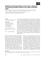
thesis, we prefer to put y to the right of x instead. For example, Figure 2.1 shows a Hasse
diagram representing poset (S, R) where S = {p, q, r, s, t} and R = {(p, q), (q, r), (p, r),
(p, s), (s, t), (p, t)}. In this poset, p and q are comparable. However, q and s are
Chapter 2. Simulation Event Orderings 33

incomparable. Further, r covers q and q covers p, but r does not cover p (although p and
r are comparable). In this thesis, we use Hasse diagram to represent a simulation event
ordering where each vertex represents an event and an arrow from event x to event y
denotes that event x must be ordered before event y.

Figure 2.1: Hasse Diagram

Dilworth’s chain covering theorem shows that a poset is formed by one or more disjoint
chains using a set inclusion [TROT92]. A chain is a set where all of its elements are
comparable. The longest chain among them is called the maximum chain and its length
is the height of the poset. The dual version of Dilworth’s chain covering theorem shows
that a poset is also formed by one or more disjoint anti-chains. Anti-chain is a set where
all of its elements are incomparable. The Dilworth’s chain covering theorem and its dual

are shown in Definition 2.3 and Definition 2.4, respectively.

Definition 2.3. For a given poset (S, R), there exists a set of posets (S
i
, R
i
) such that
∀
i

S
i
⊆ S and R
i
is a chain. R
i
is the maximum chain if there is no other R
j
where j
≠
i such
that
ij
SS > . The size of the maximum chain (i.e.,
i
S ) is the height of the poset (S,
R).

Definition 2.4. For a given poset (S, R), there exists a set of posets (S
i

, R
i
) such that
∀
i

Si ⊆ S and R
i
is an anti-chain. R
i
is the maximum anti-chain if there is no other R
j
where
p
q r
s
t
Chapter 2. Simulation Event Orderings 34

j
≠
i such that
ij
SS > . The size of the maximum anti-chain (i.e.,
i
S ) is the width of
the poset (S, R).

Figure 2.2a shows the two chains that form the poset given in Figure 2.1. The maximum
chain is {p, q, r} and therefore the height of the poset is three. Similarly, the anti-chains

that form the poset are given in Figure 2.2b. The maximum anti-chain is {s, q} or {r, t}
and the width of the poset is two. Dilworth’s chain covering theorem and its dual are
used to relate the degree of event dependency and parallelism in Chapter 3.


Figure 2.2: Dilworth’s Chain Covering Theorem and Its Dual

2.2.2 Total Order and Interval Order

Researchers in poset have proposed several orders such as total order [DUSH41],
interval order [FISH88], circle order [FISH88], angle order [FISH89], tolerance order
[BOGA95], split semi-order [FISH99], etc. The special journal Order published by
Kluwer is devoted to the theory of order and its applications (see http://www.
kluweronline.com). We will discuss total order and interval order as they are relevant to
simulation event ordering. Their definitions are given in Definition 2.5 and 2.6,
respectively.
p
s
t
p
q r
s
t
a)
q r
b)
Chapter 2. Simulation Event Orderings 35

Definition 2.5. A relation R over S is called a total order if there exists a function f for
all x∈S such that every x is mapped onto a unique n∈

Ν
, where
Ν
is the set of natural
numbers. Hence, for all x,y∈S, x is ordered before y if and only if f(x) < f(y).

Every element of S in total order is mapped onto a unique natural number. Therefore, as
the name implies, the elements of S can be arranged totally such that every two distinct
elements are comparable. For example, given S = {a, b, c} and R = {(a, b), (b, c), (a,
c)}, the order R is a total order. An order “less than” on a set of integers is another
example of total order because every integer is comparable to other integers.

Definition 2.6. Let a function I be assigned to each x∈S such that I(x) = [start(x),
end(x)], where
∀
x∈S • start (x) ≤ end (x). A relation R over S is called an interval
order if
∀
x,y∈S • (x, y) ∈ R ↔ end (x) < start (y)

Interval order assigns an interval I to each of its elements. Two distinct elements x and y
are comparable if their intervals do not intersect, i.e., I(x) ∩ I(y) = ∅. There is a special
case where the interval length, i.e., end(x) – start(x), is a constant for all x∈S. This order
is called semi-order [PIRL97]. Interval order models inexact measurement, for
examples: task scheduling where each task completion time is uncertain, or the time
spans over which animal species are found in archaeological strata, etc.

2.3 Definition of Simulation Event Orderings

Based on poset, we formalize simulation event ordering in Definition 2.7 [TEO01,

TEO04]. Just as a poset has two components (Definition 2.2), a simulation event
Chapter 2. Simulation Event Orderings 36

ordering (referred to as event ordering in short) also comprises two main components: a
set of events and an event order.

Definition 2.7. A simulation event ordering is a tuple (E, S
R
) where E is a set of events
and S
R
is a set of comparable events based on simulation event order R.

The set of comparable events S
R
is represented as a set of pairs where a pair (x, y)∈ S
R

denotes event x is ordered before event y in event order R. In simulation, we never say
that an event x is ordered before itself (i.e., (x, x) ∉ S
R
). This shows that the event
ordering uses a strong inclusion definition of poset because a weak inclusion definition
imposes that (x, x) ∈ S
R
must hold [NEGG98]. Therefore, an event order R must be anti-
reflexive, anti-symmetric, and transitive as in the strong inclusion definition of poset.

Definition 2.8. An event order R is:
1.

∀
x∈E • (x, x) ∉ S
R
(anti-reflexive)
2. (x, y) ∈ S
R
then (y, x) ∉ S
R
, and vice versa (anti-symmetric)
3. (x, y) ∈ S
R
and (y, z) ∈ S
R
then (x, z) ∈ S
R
(transitive).

2.3.1 Physical System

Simulation can adopt different event orderings to simulate a physical system provided
that the simulation result is the same as if we simulate it using the event ordering of the
physical system. Before we discuss the event ordering in the physical system, it is
important to introduce the concept of causal dependency [FUJI00]. The causal
dependency among events is based on the relation happened before [LAMP78]. An
Chapter 2. Simulation Event Orderings 37

event is dependent on another event if they happen at the same service center (i.e., access
the same resource) and one of them happens before the other. An event is also dependent
on other event, if one of them triggers the other. The two conditions are reflected in the
definition of predecessor and antecedent given below [FUJI99].


Definition 2.9. Let x be an event and x.t the physical time when event x happens. Event
x is the predecessor of y (denoted by y.pred = x), if x and y occur at the same service
center with x.t < y.t and there is no other event z that is also at the same service center
such that x.t < z.t < y.t.

Definition 2.10. Let x be an event. Event x is the antecedent of y (denoted by y.ante =
x), if x spawns y.

Figure 2.3a shows a physical system with four service centers, S
1
, S
2
, S
3
, and S
4
. Figure
2.3b shows the corresponding snapshot of event occurrences. Horizontal axis represents
physical time and vertical axis represents service centers. Label
t
i
a represents the i
th

arrival event and
t
i
d represents the corresponding departure at time t. A shaded circle
represents an event arrival and unshaded one represents an event departure. The

snapshot shows that at time 0, job 1 arrives at
S
1
. Since, S
1
is idle, job 1 is processed
until time 4. Job 2 arrives at S
1
at time 2. Since S
1
is busy, this job must wait until S
1

completes job 1, and so on. A dashed arrow from x to y shows that x is the predecessor
of y; and a solid arrow from x to y shows that x is the antecedent of y. These arrows
show the causal relationship among events in the physical system. The causal relation is
transitive, i.e., if event
x causally affects event y, and event y causally affects event z,
then event
x also causally affects event z.
Chapter 2. Simulation Event Orderings 38


Figure 2.3: Causal Dependency – Physical System

An event order in the physical system corresponds to how events in the physical system
are ordered. Based on the physical time, there is only one event order for any physical
system, i.e., an event with a smaller physical time is ordered before an event with a larger
physical time (Definition 2.11). The causal dependency among events in the physical
system is reflected in the physical time when the events occur. If event x causally affects

event
y then event x happens at an earlier physical time than event y, but the converse
may not be true.

Definition 2.11.
Let x be an event in a physical system and x.t the physical time when
event x happens. The event order in any physical system dictates that for all x and y
(where x ≠ y), x is ordered before y if and only if x.t < y.t
.

S
1

S
2

S
3

S
4

0
1
a
2
2
a
4
1

d
6
6
a
9
2
d
12
6
d

5
5
a
7
3
d
8
7
a
10
9
a
11
11
a
13
12
a
14

13
a

4
4
a
7
4
d
10
10
a

13
10
d

10
8
d
Physical Time (minute)
4
3
a
0 2 4 6 8 10 12 14
Service Center
S
1

S

2

S
3

S
4

a)
b)
      
8
8
a

Chapter 2. Simulation Event Orderings 39

Figure 2.4 shows the Hasse Diagram of the event ordering in the physical system for the
set of events given in Figure 2.3. The arrow from event x to event y in a Hasse Diagram
indicates that event x must be ordered before event y. Since an event order is transitive,
the arrows can also be traversed transitively. For example, if event x must be ordered
before event
y and event y must be ordered before event z, then event x must also be
ordered before event
z.


Figure 2.4: Hasse Diagram – Physical System

2.3.2 Simulation Model


In the Virtual Time simulation modeling paradigm [JEFF85], a simulation model
emulates a physical system and the interaction among physical processes in the physical
system (see Figure 2.5). Each physical process in the physical system is mapped onto a
logical process (LP) in the simulation model. Each event in the simulation model
represents an event in the physical system. The simulation time of an event in the
simulation model represents the physical time of the corresponding event in the physical
system. The event ordering in a physical system can be modeled and simulated using
various event orderings to exploit different degrees of event parallelism.
0
1
a
2
2
a
4
1
d
6
6
a
9
2
d
12
6
d

11
11

a
4
4
a
8
8
a
7
3
d
4
3
a
5
5
a

7
4
d
8
7
a

10
8
d
10
9
a

13
10
d

14
13
a

13
12
a
10
10
a

Chapter 2. Simulation Event Orderings 40


Figure 2.5: Mapping between Physical System and Simulation Model

Lamport defined happened before partial order and total order [LAMP78]. He proved
that both orders are anti-reflexive, anti-symmetric, and transitive which match our
definition of simulation event order (Definition 2.8). Hence, we refer to these event
orders as partial event order and total event order, respectively. The definition of partial
event order is given in Definition 2.12. Figure 2.6 shows the Hasse Diagram of the
partial event ordering (E, S
partial
) for the set of events E in Figure 2.4.

Definition 2.12. Event x is ordered before event y in partial event order if y.pred = x or

y.ante
= x.


Figure 2.6: Hasse Diagram – Partial Event Ordering

The definition of a total event order is given in Definition 2.13. The priority function in
total event order is used to decide which event should be processed when two or more
Physical Process
Logical Process
(Physical) Event (Modeled) Event
Physical time Simulation time
Physical System
Simulation Model
0
1
a
2
2
a
4
1
d
6
6
a
9
2
d
12

6
d
5
5
a

7
3
d
8
7
a
10
9
a
11
11
a
13
12
a
14
13
a

4
4
a
7
4

d
10
10
a
13
10
d
10
8
d
4
3
a
8
8
a
Chapter 2. Simulation Event Orderings 41

events have the same timestamp. For example, two events have the same timestamp, the
event with higher priority will be executed first. Figure 2.7 shows the Hasse Diagram of
the total event ordering (E, S
total
) for the set of events E in Figure 2.4.

Definition 2.13. Event x is ordered before event y in total event order if and only if:
1.
x.timestamp < y.timestamp, or
2.
x.timestamp = y.timestamp and priority(x) < priority(y).



Figure 2.7: Hasse Diagram – Total Event Ordering

Teo et al. proposed time-interval (TI) event order based on the interval order in poset
[TEO01]. Each event is assigned a time interval, with the event timestamp as the starting
point and the timestamp plus a constant W as the ending point, where W is the window
size. Definition 2.14 formalizes TI event order. Figure 2.8 shows the Hasse Diagram of
the TI event ordering (E, S
ti(4)
) with a window size of four for the set of events E given in
Figure 2.4.

Definition 2.14. Event x is ordered before event y in Time-interval (TI) event order if
y.pred
= x or y.ante = x or x.timestamp + W < y.timestamp.

TI order is similar to partial event order with a time window. In addition to the ordering
rules of partial event order (Definition 2.12), TI event order imposes that an event
x is
0
1
a
2
2
a
4
1
d
4
3

a

4
4
a
13
12
a
13
10
d
12
6
d
14
13
a

Chapter 2. Simulation Event Orderings 42

ordered before event y if x belongs to a time window that is earlier than the time window
of y and their intervals do not intersect. Therefore, if we increase the window size until a
certain value, TI event order will become partial event order as shown in Theorem 2.1.

Figure 2.8: Hasse Diagram – Time-interval Event Ordering

Theorem 2.1. For a given set of events E, ∃c such that W > c > 0 where a time-interval
(TI) event order will become a partial event order.
Proof. To prove this, we show that if W > c > 0, the third rule of TI event order (i.e.,
x.timestamp + W < y.timestamp) is redundant. Let a and b be two distinct events in E

where
b.pred ≠ a and b.ante ≠ a and b.timestamp – a.timestamp = c is the largest. If
window size
W > c, then rule x.timestamp + W < y.timestamp will produce an empty set.
Hence, only the first two rules (y.pred = x and y.ante = x) will be used, resulting in TI
event order with W > c and partial event order producing exactly the same event
ordering. For example, if we use W > 9, the links such as
0
1
a -
4
3
a ,
0
1
a -
4
4
a , and
5
5
a -
9
2
d are
not comparable (these links will not appear in Figure 2.8) and results in the same event
ordering as partial event order (see Figure 2.6). 

0
1

a
2
2
a
4
1
d
6
6
a
9
2
d
12
6
d

5
5
a
8
7
a
10
9
a

11
11
a

13
12
a
14
13
a
4
4
a
7
4
d
10
10
a
13
10
d
10
8
d

4
3
a

8
8
a
7

3
d
Chapter 2. Simulation Event Orderings 43

Timestamp (TS) event order is a special case of time-interval event order with a window
size W equal to zero [TEO01]. Hence, an event x is ordered before y if and only if
x.timestamp is smaller than y.timestamp (Definition 2.15). Figure 2.9 shows the Hasse
Diagram of the TS event ordering (E, S
ts
) for the set of events E given in Figure 2.4.

Definition 2.15. Event x is ordered before event y in timestamp (TS) event order if and
only if x.timestamp
< y.timestamp.


Figure 2.9: Hasse Diagram – Timestamp Event Ordering

2.4 Formalization

A simulator is the implementation of a simulation model. A simulator can be
implemented as a sequential program or a parallel program. The sequential simulation
maintains its event ordering by using a global event list called future event list (FEL).
Parallel simulation may employ several distributed event lists (EL) and a synchronization
algorithm (or simulation protocol) is required to maintain its event ordering. For
example, in the CMB protocol, null-messages are introduced.

0
1
a

2
2
a
4
1
d
6
6
a
9
2
d
12
6
d

8
7
a
10
9
a
11
11
a
13
12
a
14
13

a

4
3
a
5
5
a
4
4
a
7
4
d
10
10
a
13
10
d

8
8
a
10
8
d
7
3
d

Chapter 2. Simulation Event Orderings 44

In this section, we shall extract and formalize the event ordering of a number of
simulators based on poset. These include sequential simulation and some parallel
simulation protocols (such as CMB [CHAN79], Bounded Lag [LUBA89], Time Warp
[JEFF85], and Bounded Time Warp [TURN92]).

To show how a simulator executes events during runtime, for simplicity, in this section
we assume that each event requires one wall-clock time unit to execute, zero
communication delay, and for the parallel simulator each logical process (LP) is mapped
onto one physical processor (PP).

2.4.1 Sequential Simulation

The sequential simulation algorithm is presented in Figure 2.10. Events in sequential
simulation are totally ordered (only one event is executed at any time). To enforce this
ordering, sequential simulation maintains a future event list (FEL) where events are
sorted in chronological timestamp order. FEL enables sequential simulation to execute
an event with the smallest timestamp (line 12). In case of a tie (i.e., M ≠ ∅ in line 14), it
will return an event with the highest priority (z in line 15). Issues and examples on
implementing the priority function have been studied in [MEHL92, WIEL97, RONN99].

Assuming we use a priority function that assigns the highest priority to the earliest event
that is created, Figure 2.11 shows how this sequential simulation executes the events
given in Figure 2.4. Lemma 2.1 proves that events in a sequential simulation are
executed according to a total event order [TEO04]. The arrow from event x to event y is
added in the figure to indicate that event
x must be ordered before event y.
Chapter 2. Simulation Event Orderings 45



SEQUENTIAL SIMULATION
1. initialize
2. while (~stop) {
3. e ← f()
4. local_clock ← e.timestamp
5. FEL ← FEL – {e}
6. E ← execute (e)
7. FEL ← FEL ∪ E
8. stop ← g()
9. }
10.
11. f():event {
12. x ← head(FEL)
13. M ← {y | ∀y∈FEL • y.timestamp = x.timestamp}
14. if (M = ∅) return x
15. else return {z|∀y∈M ∃!z∈M • priority(z)>priority(y)}
16. }


Figure 2.10: Algorithm of Sequential Simulation


Figure 2.11: Event Execution – Sequential Simulation

Lemma 2.1. Sequential simulation implements a total event order.
Proof. Sequential simulation employs a global event list that is sorted by the smallest
timestamp first. This guarantees that event
x is ordered before event y if and only if x.ts <
y.ts. The use of a priority function when more than one event have the smallest

timestamp guarantees that if x.ts = y.ts event x is ordered before event y if and only if
priority(x) < priority(y). Therefore, events in a sequential simulation are executed
according to the total event order defined in Definition 2.13. 

2
2
a
4
1
d
4
3
a

13
12
a
13
10
d
12
6
d
0
1
a
4
4
a
14

13
a

160 170 180 190
0 10 20 30 40
Wall-clock Time
    
   
Chapter 2. Simulation Event Orderings 46

2.4.2 CMB Protocol

The algorithm of the CMB protocol [CHAN79] is given in Figure 2.12. Each LP
maintains a list of LPs that may send events to it (for LP x, it is denoted by SENDER(x)).
The ordering rule of CMB protocol imposes that only safe events can be executed. An
event in LP x is safe for execution if no other LP ∈ SENDER(x) will send any event with
a smaller timestamp to LP x. Therefore, to maintain this ordering, LP x must wait for
other LP ∈ SENDER(x) to send their events (see line 5). This blocking mechanism may
lead into a deadlock, therefore null messages are used to solve this problem. Each null
message is stamped with a timestamp ts which is equal to LP’s local simulation clock
plus a lookahead value (line 13) to indicate that the sending LP will never transmit any
events with a smaller timestamp than ts.

Static communication channels are built based on the SENDER list of each LP. The
CMB protocol assumes an order-preserving communication channel where events that
are sent through a channel will be received in the same order. The local clock, state
variables, queues, and event list (EL) of each LP are then initialized. Finally, all LPs are
activated. LPs are numbered from 0 to n-1, where n is the number of LPs. Each LP
maintains a set of input buffers (IB) and a set of output buffers (OB). IB[i] of an LP x
stores the incoming message from LP

i
∈ SENDER(x). OB[i] stores the messages that
will schedule events in LP
i
.

An LP is blocked if at least one of its IBs is empty (line 5). In lines 6-7, an event with
the smallest
f (x) is chosen from the IBs and EL of the LP for execution. Function f is the
same function that is used in the sequential simulation in Figure 2.10. Therefore, each
Chapter 2. Simulation Event Orderings 47

LP actually applies a total event order to events that are scheduled on it. Line 8 removes
the chosen event from the corresponding list (one of the IBs or EL). The local clock is
updated in line 9. In line 10, event execution may schedule a set of internal events (IE)
and a set of external events (EE). The internal events are saved to EL (line 11), and
external events to their respective
OBs (line 12). Line 13 prepares a null message with a
timestamp equal to the local clock plus a lookahead value. Lines 14-15 add a null
message to any empty
OB. Line 17 sends all the external events and null messages in the
OBs. Finally, line 18 checks the stopping condition.

CMB PROTOCOL
1. setup static channels for each communicating LP
2. initialize LPs
3. run all LPs

LOGICAL PROCESS


4. while (~stop) {
5. while (∃i IB[i] = ∅) {}
6. L ← EL ∪ {Ui IB[i]}
7. e ← f()
8. if (∃i e∈IB[i]) IB[i] ← IB[i]–{e} else EL ← EL–{e}
9. local_clock ← e.timestamp
10. {IE, EE} ← execute (e)
11. EL ← EL ∪ IE
12. ∀i OB[i] ← OB[i] ∪ {z | z∈EE • z.lp = i}
13. nullMsg.timestamp ← local_clock + lookahead
14. for i←0 to n-1 do {
15. if (OB[i] = ∅) OB[i] ← OB[i] ∪ {nullMsg}
16. }
17. ∀i send (OB[i])
18. stop ← g()
19.}

Figure 2.12: Algorithm of the CMB Protocol

Assuming a lookahead of 1, Figure 2.13 shows how the CMB protocol executes events
in Figure 2.3. For simplicity, we do not show the null messages. During initialization,
events
0
1
a ,
4
3
a
, and
4

4
a are created at the respective LPs. LP
1
and LP
3
have no
Chapter 2. Simulation Event Orderings 48

dependency on other LPs (their SENDER list = ∅); hence, they can execute the events
received right away. LP
1
executes event
0
1
a and schedules events
2
2
a and
4
1
d . At the
same time, LP
3
executes event
4
4
a and schedules events
7
4
d and

10
10
a . LP
2
cannot execute
event
4
3
a
because there is no guarantee from LP
1
that it will not send events with a
timestamp less than 4. Next, LP
1
executes event
2
2
a while LP
3
executes event
7
4
d . The
executions produce events
6
6
a and
8
7
a . At this time, a null message is sent from LP

1
to
LP
2
that it will not send any event with a timestamp earlier than five. It LP
1
guarantees
that event
4
3
a is safe. Hence event
4
3
a can be executed in parallel with events
4
1
d and
10
10
a
at timestep 2. This process continues until the simulation completes the execution of
event
14
13
a . Lemma 2.2 shows the event ordering implemented by the CMB protocol
[TEO04].

Figure 2.13: Event Execution– the CMB Protocol

Lemma 2.2. CMB protocol implements an event order whereby event x is ordered

before event y if:
1.
y.pred = x, or
LP
1

LP
2

LP
3

LP
4

0
1
a
Wall-clock Time
0 1 2 3 4 5 6 7 8 9
Logical Process
5
5
a
7
3
d
8
7
a

10
9
a
11
11
a
13
12
a
14
13
a
2
2
a
4
1
d
12
6
d
9
2
d
6
6
a
4
4
a

10
10
a
8
8
a
7
4
d
13
10
d
10
8
d
         
4
3
a
Chapter 2. Simulation Event Orderings 49

2. x.lp ∈ SENDER(y.lp) and x.timestamp + lookahead < y.timestamp
Proof. The blocking mechanism (line 5) ensures that an LP has to wait until all LPs in
its SENDER list have sent their events. This ensures that an LP always executes events
scheduled in it in timestamp order. Hence, for all events in the same LP, if y.pred = x
then x is ordered before y. Further, event y in LP
j
is executed only if it has the smallest
timestamp among the unprocessed events of all LP ∈ SENDER(LP
j

). Therefore, event x
in any LP ∈ SENDER(LP
j
) is ordered before event y only if x.timestamp + lookahead <
y.timestamp where lookahead is the lookahead value. 

Researchers have proposed various optimizations of the original CMB protocol such as:
the demand driven protocol [BAIN88], flushing protocol [TEO94], and carrier null
message protocol [CAI92, WOOD94]. We shall show that these optimizations do not
alter simulation event ordering in the original CMB protocol, but rather, they can be seen
as three different implementations of the same simulation event order.

The algorithm of the demand driven protocol is similar to the algorithm of the CMB
protocol. The demand driven protocol modifies line 5 in the algorithm given in Figure
2.12. Instead of being blocked, an LP sends a request to any LP in its SENDER list from
which it has not received any event. When an LP receives a request, it sends a null
message with a timestamp equal to its local clock plus a lookahead value. Hence, instead
of sending null messages after each event execution, an LP sends a null message only
when it is “required”. Although the demand driven protocol reduces the number of null
messages, the null message still serves the same purpose as in the original CMB
protocol. Therefore, for the same set of events, the demand driven protocol will execute
the events in the same order as in the original CMB protocol.
Chapter 2. Simulation Event Orderings 50


The algorithm of the flushing protocol is also similar to the algorithm of the CMB
protocol given in Figure 2.12. When an LP receives a null message from another LP, all
unprocessed null messages with a smaller timestamp than the incoming null message at
the recipient LP will be removed. Hence, an LP only needs to process a null message
with the largest timestamp. When a null message is pumped to an OB, all unsent null

messages with a timestamp less than the new null message will be removed. Hence, an
LP only needs to send a null message with the largest timestamp. This approach reduces
the number of null messages but does not change the main part of the algorithm (lines 6-
12) that controls event ordering.

The algorithm of the carrier null message protocol is similar to that of the CMB protocol
except for the structure of the null message [CAI90, WOOD94]. The null message in the
carrier null message protocol carries routing information to shorten the circulation of null
messages on a system with cyclic topology. The change in the null message structure
definitely does not make the event ordering any different from that in the original CMB
protocol.

2.4.3 Bounded Lag Protocol

Lubachevsky proposed the Bounded Lag (BL) protocol which combines two main rules:
bounded lag restriction and minimum propagation delay [LUBA89]. Bounded lag
restriction imposes that events can be executed concurrently if they are within the same
time window. Minimum propagation delay between LPs is used to determine whether an
event is safe to execute. The latter is similar to the rule in CMB protocol, however in the
Chapter 2. Simulation Event Orderings 51

implementation BL protocol uses a distance matrix instead of using null messages. To
maintain its ordering, BL protocol uses barrier synchronization because the global clock
(for imposing bounded lag restriction) and the minimum propagation delay must be
broadcast to all LPs. The algorithm is given in Figure 2.14. There are two main
processes: the nomination of safe events (lines 7-10) and the execution of safe events
(lines 11-18).

BL PROTOCOL
1. setup static channels for each communicating LP

2. setup a distance matrix
3. initialize global_clock
4. initialize LPs
5. run all LPs

LOGICAL PROCESS

6. while (~stop) {
7. M ← {∀lp∈LP, lp≠this • head(lp.EL)}
α ← min {∀e∈M • e.timestamp+d(e.lp, this)}
broadcast α
8. barrier synchronization
9. E ← {∀e∈EL • e.timestamp ≤ min(α, global_clock+W)}
10. EL ← EL - E
11. while (E ≠ ∅) {
12. e ← head(E)
13. E ← E – {e}
14. {IE, EE} ← execute (e)
15. local_clock ← e.timestamp
16. EL ← EL ∪ IE
17. Send(EE)
18. }
19. stop ← g()
20. barrier synchronization
21. global_clock ← min {∀lp∈LP • lp.local_clock}
broadcast global_clock
22.}

Figure 2.14: Algorithm of the Bounded Lag Protocol


The BL protocol makes use of a distance matrix d to store the lookahead between any
two LPs. Based on the distance matrix, an LP (denoted by this in Figure 2.14)
determines the earliest time α when its system state can be affected by other LPs (line 7).
Chapter 2. Simulation Event Orderings 52

The barrier synchronization in line 8 ensures that all LPs calculate α before continuing to
the next line. Each LP identifies its safe events based on this rule: events with a
timestamp less than α and within a time window of
W are safe to process (line 9). Line
10 removes all safe events from EL for execution.

The BL protocol retrieves a safe event with the least timestamp in line 12 and removes it
from the list E in line 13. In line 14, event execution may schedule a set of internal
events (IE) and a set of external events (EE). The internal events will be added to the EL
(line 16) and the external events will be sent to their respective LPs (line 17). The barrier
synchronization in line 20 is used to ensure that all LPs have processed their safe events
before the time window is moved. Line 21 computes the global clock as the minimum of
all LPs’ local clock. This process is repeated until the stopping condition is met. Lemma
2.3 shows the event ordering that is implemented by the BL protocol [TEO04].

Lemma 2.3. BL protocol implements an event order whereby event x is ordered before
event y if:
1.
y.pred = x, or
2.
x.timestamp + lookahead < y.timestamp, or
3.
⎣x.timestamp/W⎦ < ⎣y.timestamp/W⎦.
Proof. The value of α in line 7 gives the smallest timestamp of an unprocessed event x
(plus lookahead) that may be sent to a particular LP (Figure 2.14). Line 9 shows that if

event y in LP
i
can be executed in parallel with event x from another LP
j
, then
y.timestamp ≤ α (i.e., x.timestamp+distance(LP
i
, LP
j
)), and both x and y must be in the
same time window of size
W (Note that the distance between LP
i
and LP
j
is the
lookahead between the two LPs). Therefore, the contra positive, i.e., event x is executed