A framework for formalization and characterization of simulation performance 4
Bạn đang xem bản rút gọn của tài liệu. Xem và tải ngay bản đầy đủ của tài liệu tại đây (262.04 KB, 40 trang )
105
Chapter 4
Experimental Results
We have proposed a framework for characterizing simulation performance from the
physical system layer to the simulator layer. In this chapter, we conduct a set of
experiments to validate the framework and to demonstrate the usefulness of the
framework in analyzing the performance of a simulation protocol.
To do experiment, first, we implement a set of measurement tools to measure the
performance metrics at the three layers. Using these measurement tools, we test the
framework. Then, we apply the framework to study the performance of Ethernet
simulation.
Experiments that are used to measure performance metrics at the physical system layer
and the simulation model layer are conducted on a single processor. Experiments using
the SPaDES/Java parallel simulator (to measure performance metrics at the simulator
layer) are conducted on a computer cluster of eight nodes connected via a Gigabit
Ethernet. Each node is a dual 2.8GHz Intel Xeon with 2.5GB RAM.
Chapter 4. Experimental Results 106
The rest of this chapter is organized as follows. First, we discuss the measurement tools
that we have developed for use in the experiments. Next, we test the proposed
framework using an open and a closed system. After that, we discuss the application of
the framework to study the performance of Ethernet simulation. We conclude this
chapter with a summary.
4.1 Measurement Tools
To apply the proposed framework, we need tools to measure event parallelism, memory
requirement, and event ordering strictness at the three different layers. We have
developed two tools to measure these performance metrics as shown in Figure 4.1.
Figure 4.1: Measurement Tools
Sequential
Time, Space and Strictness
Analyzer
SPaDES / Java
Simulator
Π
prob
, M
prob
Π
ord
, M
ord
Π
sync
, M
sync
,
M
tot
Simulation
Problem
Event Orders
Physical
System
Simulation
Model
Simulator
Layers
Metrics
Measurement Tools
Real +
overhead
events
Real
events
Mappin
g
ς
All Layers
Parallel
Chapter 4. Experimental Results 107
At the physical system layer, performance metrics (Π
prob
and M
prob
) are measured using
the SPaDES/Java simulator. At the simulation model layer, the Time, Space and
Strictness Analyzer (TSSA) is used to measure Π
ord
and M
ord
. The SPaDES/Java
simulator is also used to measure performance metrics (Π
sync
, M
sync
, and M
tot
) at the
simulator layer. Depending on the inputs, TSSA can be used to measure event ordering
strictness (ς) at the three layers. The details are discussed in the following sections.
4.1.1 SPaDES/Java Simulator
SPaDES/Java is a simulator library that supports a process-oriented worldview
[TEO02A]. We extend the SPaDES/Java to support the event-oriented worldview and
use this version in our experiments. The SPaDES/Java supports a sequential simulation
and a parallel simulation based on the CMB protocol with demand-driven optimization
[BAIN88].
The SPaDES/Java is used to simulate a simulation problem (physical system) and to
measure event parallelism (Π
prob
) and memory requirement (M
prob
) at the physical system
layer. Based on Equations 3.2 and 3.5, Π
prob
and M
prob
are derived from the number of
events and maximum queue size, respectively. Therefore, instrumentation is inserted into
the SPaDES/Java to measure the number of events and the maximum queue size of each
service center.
The SPaDES/Java is also used to measure effective event parallelism (Π
sync
), memory for
overhead events (M
sync
), and total memory requirement (M
tot
) at the simulator layer.
Chapter 4. Experimental Results 108
Based on Equation 3.4, Π
sync
is derived from the number of events and the simulation
execution time. M
sync
is derived from the size of the data structure used to store null
messages (Equation 3.7). M
tot
is derived from the size of the data structures that
implement queues, event lists and buffers for storing null messages (Equation 3.8).
Therefore, instrumentation is inserted into the SPaDES/Java simulator to measure the
number of events, the simulation execution time, and the size of data structures that
implement queues, event lists, and buffers for storing null messages.
The sequential execution of the SPaDES/Java produces a log file containing information
on the sequence of event execution that will be used by TSSA to measure time and space
performance at the simulation model layer as well as the strictness of different event
orderings at the physical system and simulation model layers. The parallel execution of
the SPaDES/Java produces a set of log files (one for every PP). Each log file contains
information on the sequence of event execution (real and overhead) in a PP. These log
files will be used by TSSA to measure the strictness of event ordering at the simulator
layer.
4.1.2 Time, Space and Strictness Analyzer
We have developed the Time, Space and Strictness Analyzer (TSSA) to simulate
different event orderings, to measure event parallelism (Π
ord
) and memory requirement
(M
ord
) at the simulation model layer, and to measure event ordering strictness (ς) at the
three layers.
Chapter 4. Experimental Results 109
To measure Π
ord
and M
ord
, TSSA needs two inputs, i.e., the log file generated by the
sequential execution of the SPaDES/Java and the event order to be simulated. Every
event executed by the SPaDES/Java is stored in a record in the log file, and the record
number indicates the sequence when the SPaDES/Java executes the event. Each record
also contains information on event dependency. Based on a given event ordering, TSSA
simulates the execution of events and measures Π
ord
and M
ord
. Based on Equation 3.3,
Π
ord
is derived from the number of events and the simulation execution time (in
timesteps). M
ord
is derived from the maximum event list size of each LP. Therefore,
TSSA is equipped with an instrumentation to measure the simulation execution time and
the maximum event list size of each LP.
To measure the strictness of event ordering (ς) at the physical system layer and the
simulation model layer, TSSA also needs the same inputs listed in the previous
paragraph. At every iteration, TSSA reads a fixed number of events from the log file,
and measures the strictness of the given event order based on Definition 3.2. This
method is used because to measure the strictness of an event ordering with a large
number of events is computationally expensive. Event ordering strictness is then derived
by summing up the strictness at every iteration, and dividing it by the number of
iterations.
To measure the strictness of event ordering (ς) at the simulator layer, TSSA requires the
log files generated by the parallel execution of the SPaDES/Java simulator. Every event
executed by the SPaDES/Java on a PP is stored in a record of a log file associated with
the PP. This includes real events as well as overhead events (i.e., null messages). From
Chapter 4. Experimental Results 110
these log files, TSSA deduces the dependency among events and uses the same method
as in the previous paragraph to measure event ordering strictness at the simulator layer.
4.2 Framework Validation
The objective of the experiments in this section is to validate our framework using an
open system called Multistage Interconnected Network (MIN) and a closed system called
PHOLD as the benchmarks. First, we validate each measurement tool that analyzes the
performance at a single layer. The results are validated against analytical results. The
validated tools are used to measure time and space performance at each layer
independent of other layers. Next, we compare the time performance across layers in
support of our theory on the relationship among the time performance at the three layers.
Next, we analyze the total memory requirement. Finally, we measure the strictness of a
number of event orderings in support of our strictness analysis in Chapter 3.
4.2.1 Benchmarks
We use two benchmarks:
1. Multistage Interconnected Network (MIN)
MIN is commonly used in a high speed switching system and it is modeled as an
open system [TEO95]. MIN is formed by a set of stages; each stage is formed by the
same number of switches. Each switch in a stage is connected to two switches in the
next stage (Figure 4.2a). Each switch (except at the last stage) may send signals to
one of its neighbors with equal probability. We model each switch as a service
Chapter 4. Experimental Results 111
center. MIN is parameterized by the number of switches (n×n) and traffic intensity
(ρ) which is the ratio between the arrival rate (λ) and the service rate (µ).
2. Parallel Hold (PHOLD)
PHOLD
is commonly used in parallel simulation to study and represent a closed
system with multiple feedbacks [FUJI90]. Each service center is connected to its
four neighbors as shown in Figure 4.2b. PHOLD is parameterized with the number
of service centers (n×n) and job density (m). Initially, jobs are distributed equally
among the service centers, i.e., m jobs for each service center. Subsequently, when a
job has been served at a service center, it can move to one of the four neighbors with
an equal probability.
Figure 4.2: Benchmarks
Table 4.1 shows the total number of events that occur during an observation period of
10,000 minutes for both physical systems. All service centers in both MIN and PHOLD
have the same service rates. The table shows that for MIN, the total number of events
depends on the problem size and traffic intensity. From Little’s law [JAIN91], at steady
state condition, the number of jobs that arrive at a service center is equal to the job
a
)
MIN
(
3×3
,
ρ
)
b)
PHOLD
(
3×3
,
m
)
Chapter 4. Experimental Results 112
arrival rate (λ) multiplied by the observation period (D). Since each job in MIN and
PHOLD generates two events (arrival and departure), the number of events (||E||) at a
service center is ||E|| = 2 × λ × D. Since ρ = λ / µ, ||E|| = 2 × ρ × µ × D, where µ is the
service rate of each service center. Therefore, for n × n service centers, the number of
events can be modeled as:
||E|| = 2 × ρ × µ × D × n × n (4.1)
MIN PHOLD
Problem size
ρ
Number of events m Number of events
0.2 52,156 1 132,437
0.4 103,981 4 222,384
0.6 161,376 8 249,584
8×8
0.8 220,431 12 261,675
0.2 205,964 1 525,411
0.4 427,924 4 886,191
0.6 640,067 8 999,156
16×16
0.8 868,465 12 1,045,912
0.2 468,002 1 1,176,686
0.4 946,792 4 1,991,927
0.6 1,455,067 8 2,246,027
24×24
0.8 1,941,903 12 2,351,078
0.2 824,529 1 2,093,555
0.4 1,679,004 4 3,541,933
0.6 2,536,016 8 4,004,896
32×32
0.8 3,405,761 12 4,178,760
Table 4.1: Characteristics of the Physical System
The table also shows that the total number of events for PHOLD depends on the problem
size and message density. All service centers in both MIN and PHOLD have the same
service rates. Based on forced flow law, the arrival rate of a closed system is equal to its
throughput [JAIN91]. Further, based on interactive response time law [JAIN91], the
throughput of a closed system is a function of message density (m). Appendix C shows
that message density has a logarithmic effect on traffic intensity in PHOLD. Hence, for
Chapter 4. Experimental Results 113
PHOLD, Equation 4.1 can be rewritten as the following equation where c
1
and c
2
are
constants.
||E|| = 2 × (c
1
× log (c
2
+ m)) × µ × D × n × n (4.2)
4.2.2 Physical System Layer
The objective of this experiment is to measure time and space performance at the
physical system layer (Π
prob
and M
prob
). First, we validate the SPaDES/Java simulator
that is used to measure Π
prob
and M
prob
. We run the SPaDES/Java simulator to obtain the
throughput and average queue size of the two physical systems (i.e., MIN and PHOLD).
The results are validated against analytical results based on queuing theory and mean
value analysis. The validation results show that there is no significant difference
between the simulation results and the analytical results. The detail validation process
can be seen from Appendix B. Next, we use the validated SPaDES/Java simulator to
measure Π
prob
and M
prob
of the two physical systems. Figure 4.3 and Figure 4.4 show the
event parallelism (Π
prob
) of MIN and PHOLD, respectively. The detail experimental
results in this chapter can be found in Appendix C.
Figure 4.3 shows that the event parallelism (Π
prob
) of MIN varies with problem size
(n×n) and traffic intensity (ρ). The result confirms that a bigger problem size (more
service centers) and higher traffic intensity increase the number of events per time unit
(Equation 4.1). Figure 4.4 shows the effect of a varying problem size (n×n) and message
intensity (m) on the event parallelism (Π
prob
) of PHOLD. The result confirms that a
bigger problem size and higher message density increase the number of events that occur
per unit of time (Equation 4.2).
Chapter 4. Experimental Results 114
0
50
100
150
200
250
300
350
400
450
8x8 16x16 24x24 32x32
Problem size (nxn)
p=0.8
p=0.6
p=0.4
p=0.2
Π
prob
(events/minute)
Figure 4.3: Π
prob
– MIN (n×n, ρ)
0
50
100
150
200
250
300
350
400
450
8x8 16x16 24x24 32x32
Problem size (nxn)
m=12
m=8
m=4
m=1
Π
prob
(events/minute)
Figure 4.4: Π
prob
– PHOLD (n×n, m)
Chapter 4. Experimental Results 115
The memory requirement of the physical system MIN (M
prob
) under a varying problem
size (n×n) and traffic intensity (ρ) is shown in Figure 4.5. The figure suggests that M
prob
depends on problem size and traffic intensity. As shown in Chapter 3, we derive M
prob
from the queue size at each service center. Hence, an increase in the number of service
centers (problem size) increases M
prob
. The same observation can also be made at
PHOLD (Figure 4.6).
In MIN, high traffic intensity means that the service centers have to cope with many
jobs. Similarly, in PHOLD, high message density indicates that the system has more
jobs to execute. Consequently, a physical system with higher traffic intensity or message
density requires more memory because the size of its queues is longer.
0
5
10
15
20
25
8x8 16x16 24x24 32x32
Problem size (nxn)
p=0.8
p=0.6
p=0.4
p=0.2
Μ
prob
(thousands unit)
Figure 4.5: M
prob
– MIN (n×n, ρ)
Chapter 4. Experimental Results 116
0
5
10
15
20
25
30
35
40
45
8x8 16x16 24x24 32x32
Problem size (nxn)
m=12
m=8
m=4
m=1
Μ
prob
(thousands unit)
Figure 4.6: M
prob
– PHOLD (n×n, m)
4.2.3 Simulation Model Layer
The objective of this experiment is to measure the time and space performance of
different event orderings at the simulation model layer (Π
ord
and M
ord
). First, we validate
TSSA, and then use the validated TSSA to measure event parallelism exploited by
different event orders (Π
ord
) and their memory requirement (M
ord
).
Wang et al. developed an algorithm to predict the upper bound of model parallelism (or
Π
ord
in our framework) [WANG00]. Therefore, we validate the parallelism of partial
event ordering produced by our TSSA against the result of the algorithm. The results
show that the algorithm gives an upper bound on Π
ord
produced by TSSA. The detail is
given in Appendix A.
Chapter 4. Experimental Results 117
Next, we use the validated TSSA to measure Π
ord
and M
ord
. Figure 4.7 and Figure 4.8
show that Π
ord
depends on problem size (n×n), traffic intensity (ρ), and the event order
used.
A physical system with a bigger problem size and higher traffic intensity would have to
handle more events within the same duration than a physical system with a smaller
problem size and lower traffic intensity. Hence, more events can potentially be
processed at the same time. At the same time, different event orders impose different
ordering rules which also affect the number of events that can be executed at the same
time. The result confirms that for the same duration, a stricter event order will never
execute more events than the less strict event order (see Theorem 3.9). In this open
system example, the partial event order and the CMB event order exploit almost the
same amount of parallelism; therefore, only one line can be seen from Figure 4.7 and
Figure 4.8.
0
100
200
300
400
500
600
700
800
8x8 16x16 24x24 32x32
Problem size (nxn)
Partial
CMB
TI(5)
TS
Total
Π
ord
(events/timestep)
Figure 4.7: Π
ord
– MIN (n×n, 0.8)
Chapter 4. Experimental Results 118
0
10
20
30
40
50
60
0.2 0.4 0.6 0.8
Traffic intensity (p)
Partial
CMB
TI(5)
TS
Total
Π
ord
(events/timestep)
Figure 4.8: Π
ord
– MIN (8×8, ρ)
Figure 4.9 and Figure 4.10 show the event parallelism (Π
ord
) of different event orders in
simulating PHOLD. The result shows that Π
ord
varies with the problem size (n×n),
message density (m), and event order. The problem size and event order affect Π
ord
for
the same reason as in the open system example. An increase in message density (m)
improves parallelism (Π
ord
). This is because high message density increases the
probability that each LP has some events to process at any given time. The improvement
levels off eventually when each LP has an event to process at all times. The result also
confirms that for the same duration, a stricter event order will never execute more events
than a less strict event order (Theorem 3.9).
Chapter 4. Experimental Results 119
0
50
100
150
200
250
300
350
400
450
8x8 16x16 24x24 32x32
Problem size (nxn)
Partial
TI(5)
CMB
TS
Total
Π
ord
(events/timestep)
Figure 4.9: Π
ord
– PHOLD (n×n, 4)
0
5
10
15
20
25
30
35
14812
Message density
Partial
TI(5)
CMB
TS
Total
Π
ord
(events/timestep)
Figure 4.10: Π
ord
– PHOLD (8×8, m)
We can observe from Figure 4.8 and Figure 4.9 that the event parallelism of CMB is
better than that of TI(5) for the MIN problem, but the event parallelism of TI(5) is better
Chapter 4. Experimental Results 120
than that of CMB for the PHOLD problem. This is because time-interval event order is
not comparable to the event order in CMB protocol as shown in Figure 3.8. Therefore, it
is possible that time-interval event order can exploit more parallelism than the event
order of CMB protocol at some problems but exploiting less parallelism at other
problems.
We can also observe that the same event order may exploit different degrees of Π
ord
from
two different physical systems with the same Π
prob
. Figure 4.3 and Figure 4.4 show that
for the same problem size, the inherent event parallelism (Π
prob
) of MIN with ρ = 0.8 is
not significantly different from the inherent event parallelism of PHOLD with m = 4 (this
is also supported by the analytical results shown in Appendix C). However, the same
event order exploits more event parallelism at the simulation model layer (Π
ord
) when it
is used in MIN than when it is used in PHOLD (compare Figure 4.7 and Figure 4.9).
This is caused by the difference in the topology of the two physical systems. At the
simulation model layer, we can execute events at different LPs in parallel as long as they
are independent. MIN generates less dependent events than PHOLD because of the
multiple feedbacks in PHOLD. Therefore, at the simulation model layer, the same event
order can exploit more parallelism (Π
ord
) from MIN than PHOLD.
Table 4.2 shows the (maximum) memory requirement (M
ord
) of different event orders in
simulating MIN, and Table 4.3 shows the respective average memory requirement. As in
Π
ord
, the memory requirement (M
ord
) varies with the problem size (n×n), traffic intensity
(ρ), and the event order used. More events occur within the same duration in a system
with a bigger problem size and higher traffic intensity. Hence, more memory is required
Chapter 4. Experimental Results 121
to store these events. A less strict event order also tends to exploit more parallelism
(Π
ord
) than a stricter one.
Problem size (n×n)
Traffic intensity (ρ)
Event
Order
8×8 16×16 24×24 32×32
Event
Order
0.2 0.4 0.6 0.8
Partial 2,145 8,151 16,516 27,722 Partial 1,073 1,551 1,964 2,145
CMB 2,165 8,198 16,642 27,909 CMB 1,076 1,556 1,970 2,165
TI(5) 302 1,192 2,646 4,652 TI(5) 185 226 259 302
TS 92 301 656 1,102 TS 37 56 75 92
Total 88 296 640 1,093 Total 35 53 73 88
Table 4.2: M
ord
– MIN
Problem size (n×n)
Traffic intensity (ρ)
Event
Order
8×8 16×16 24×24 32×32
Event
Order
0.2 0.4 0.6 0.8
Partial 879 2,822 5,164 7,766 Partial 371 625 756 879
CMB 888 2,845 5,234 7,903 CMB 375 629 763 888
TI(5) 73 268 589 1,016 TI(5) 23 38 55 73
TS 68 253 561 975 TS 22 36 52 68
Total 64 245 376 958 Total 21 36 50 64
Table 4.3: Average Memory Requirement – MIN
The (maximum) memory requirement (M
ord
) and average memory requirement of
different event orders in simulating PHOLD are shown in Table 4.4 and Table 4.5,
respectively.
Table 4.4 shows that as the message density gets higher (m ≥ 8), the value of M
ord
tends
to converge to the same value. The explanation is as follows. From the extreme values
theory, the probability that a maximum number of events will exceed a threshold
depends on the value of the threshold, the average number of events, and the standard
deviation [COLE01]. A high threshold value, low average number of events, and narrow
standard deviation result in a smaller probability. In PHOLD, initially, n×n×m events are
a)
ρ
= 0.8
b) Problem Size = 8×8
a)
ρ
= 0.8
b) Problem Size = 8×8
Chapter 4. Experimental Results 122
distributed evenly among n×n LPs (m events per LP). This sets a threshold value of m.
Therefore, the probability of the maximum number of events in each LP exceeding m
depends on the average number of events and its standard deviation. For partial event
ordering with a large m = 8 and 12, the average number of events per LP is only 1.5
(97/64) and 1.6 (103/64), respectively. The standard deviation is only 0.16 and 0.65,
respectively. Therefore, statistically, as we increase m, it becomes more unlikely that the
maximum number of events per LP will exceed m. It is even less likely for the less strict
event orderings.
Problem size (n×n)
Traffic intensity (ρ)
Event
Order
8×8 16×16 24×24 32×32
Event
Order
1 4 8 12
Partial 468 1,878 4,245 7,584 Partial 359 468 532 770
CMB 305 1,237 2,836 4,892 CMB 252 305 514 770
TI(5) 321 1,299 2,736 4,952 TI(5) 261 321 515 770
TS 256 1,024 2,304 4,096 TS 64 256 512 768
Total 256 1,024 2,304 4,096 Total 64 256 512 768
Table 4.4: M
ord
– PHOLD
Problem size (n×n)
Traffic intensity (ρ)
Event
Order
8×8 16×16 24×24 32×32
Event
Order
1 4 8 12
Partial 84 338 761 1354 Partial 45 84 97 103
CMB 66 260 580 1026 CMB 39 66 75 78
TI(5) 67 265 596 1060 TI(5) 39 67 76 80
TS 62 245 551 979 TS 37 62 69 73
Total 58 229 512 912 Total 34 58 65 67
Table 4.5: Average Memory Requirement – PHOLD
Table 4.5 shows that the average memory requirement depends on the problem size
(n×n) and event order for the same reason as in the MIN example. Message density (m)
a) m = 4
b) Problem Size = 8×8
a) m = 4
b) Problem Size = 8×8
Chapter 4. Experimental Results 123
also affects the average memory requirement because a higher message density implies
that more events are generated.
4.2.4 Simulator Layer
In this section, we measure performance metrics (Π
sync
and M
sync
) at the simulator layer.
We use the SPaDES/Java simulator in this experiment. As discussed in Chapter 1, many
factors affect the performance of a simulator at runtime. In this experiment, we do not
attempt to study all factors that affect Π
sync
and M
sync
, but we demonstrate how
performance is measured at the simulator layer so as to complete our three layered
performance characterization.
We map a number of service centers (each is modeled as a logical process) onto a
physical processor (PP). To reduce the null message overhead, logical processes (LPs)
that are mapped onto the same PP communicate via shared memory. Java RMI is used
for inter-processor communication among LPs that are mapped onto different processors.
We run our SPaDES/Java parallel simulator on four and eight PPs. The results are
shown in Figure 4.11 and Figure 4.12.
Figure 4.11 shows that effective event parallelism (Π
sync
) is affected by the number of
LPs. For the same number of PP, the result shows that an increase in the number of LPs
increases the exploited parallelism. This can be explained by comparing Figure 4.3 and
Figure 4.12a. Both figures show that an increase in the number of LPs increases the
number of useful events and null messages at different rates. The rate of increase in the
useful events is higher than that of the null messages. Therefore, the proportion of time
Chapter 4. Experimental Results 124
that is spent by the processors to execute useful events increases as the number of LPs
increases. Consequently, it increases the exploited parallelism.
0
5000
10000
15000
20000
25000
8x8 16x16 24x24 32x32
Problem Size
8PP
4PP
Π
sync
(events/second)
0
2000
4000
6000
8000
10000
12000
8x8 16x16 24x24 32x32
Problem Size
8PP
4PP
Π
sync
(events/second)
Figure 4.11: Π
sync
– a) MIN (n×n, 0.8) and b) PHOLD (n×n, 4)
The experimental also shows that Π
sync
is affected by the number of PPs. An increase in
the number of PPs increases computing power so that less time is spent in executing
useful events. At the same time, it increases the number of null messages to synchronize
more PPs. The result shows that an increase from four PPs to eight PPs improves the
parallelism because the reduction of time for executing useful events are higher than the
a)
b)
Chapter 4. Experimental Results 125
additional time to execute extra null messages. Since the number of null messages
increases exponentially with the number of PPs (Figure 12), further increase in the
number of PPs will eventually decrease the exploited event parallelism.
0
500
1000
1500
2000
2500
3000
3500
8x8 16x16 24x24 32x32
Problem Size
8PP
4PP
Μ
sync
(unit)
0
1000
2000
3000
4000
5000
6000
8x8 16x16 24x24 32x32
Problem Size
8PP
4PP
Μ
sync
(unit)
Figure 4.12: M
sync
– a) MIN (n×n, 0.8) and b) PHOLD (n×n, 4)
In the CMB protocol, M
sync
is derived from the maximum number of null messages for
all PPs. For the same problem size, an increase in the number of PPs increases the
number of null messages because more overhead is needed to synchronize more PPs.
For the same number of PPs, an increase in the problem size (i.e., the number of LPs)
a)
b)
Chapter 4. Experimental Results 126
may result in more communication channels among LPs (at different PPs). This
increases the number of null messages that must be sent. The result shows that more null
messages are generated in PHOLD than in MIN because of the feedback in PHOLD.
4.2.5 Parallelism Analysis
In this section, we first show the parallelism profile exploited by the SPaDES/Java for
the two benchmarks. Next, we normalize event parallelism using the method that has
been explained in Chapter 3, and compare the normalized event parallelism.
The parallelism profile of MIN and PHOLD are shown in Figure 4.13 and Figure 4.14,
respectively. The horizontal axis is the wall-clock time, and the vertical axis is event
parallelism (the number of events executed per second). The profiles show that MIN has
more parallelism than PHOLD.
0
5000
10000
15000
20000
25000
30000
0 50 100 150 200 250 300
Wall-clock Time (s)
Π
sync
(events/second)
Figure 4.13: Parallelism Profile – MIN (32×32, 0.8)
Chapter 4. Experimental Results 127
0
2000
4000
6000
8000
10000
12000
14000
16000
0 100 200 300 400 500 600
Wall-clock Time (s)
Π
sync
(events/second)
Figure 4.14: Parallelism Profile – PHOLD (32×32, 4)
Next, we normalize and compare event parallelism at the three layers. The results are
shown in Figure 4.15 and Figure 4.16. The normalization results are consistent with the
previous results for each layer. First, the normalized event parallelism increases as the
problem size increases. Second, at the simulation model layer, for the same level of
Π
ord
, CMB event order exploits more parallelism from MIN than PHOLD. Third, at the
simulator layer, the SPaDES/Java exploits more parallelism when it is used to simulate
MIN than when it is used to simulate PHOLD.
57
211
451
766
8
26
51
83
5.83
5.97
6.04 6.11
1
10
100
1000
8x8 16x16 24x24 32x32
Problem Size
Prob
Ord
Sync
Π
norm
Figure 4.15: Normalized Parallelism– MIN (n×n, 0.8)
Chapter 4. Experimental Results 128
22
79
176
313
9
26
51
83
1.26
1.94
2.31
2.56
1
10
100
1000
8x8 16x16 24x24 32x32
Problem Size
Prob
Ord
Sync
Π
norm
Figure 4.16: Normalized Parallelism– PHOLD (n×n, 4)
The comparison results show that event parallelism at the physical system layer can be
exploited by the CMB event order at the simulation model layer. However, the
implementation overheads reduce the event parallelism at the simulator layer.
4.2.6 Total Memory Requirement
In this section, we analyze the total memory required by the SPaDES/Java to simulate
the two benchmarks. First, we show the memory profiles for simulating MIN and
PHOLD in Figure 4.17 and Figure 4.18, respectively. The horizontal axis shows the
wall-clock time in 100ms (logarithmic scale). We choose 100ms so that we can observe
the fluctuation more accurately. The vertical axis shows the required memory in unit
(i.e., the number of entries in the data structures that implement queues, event lists and
buffers for storing null messages). The profiles show that the queues (that are used to
derive M
prob
) are initially empty and increase until a certain level. In MIN, an event is
scheduled for each LP in the first stage (leftmost column in Figure 4.2a). Therefore,
initially, for n×n MIN, n events are in the event lists (that are used to derive M
ord
). The
profile shows that the total number of events in the event lists increases until a certain
Chapter 4. Experimental Results 129
level. In PHOLD, m events are scheduled for each LP before the simulation starts.
Therefore, initially, for n×n PHOLD, more events (n×n×m) are in the event lists than in
MIN. The profile shows that the total number of events in the event lists decreases until a
certain level. This confirms the memory profile reported in [TEO01]. The profiles show
that the null message population (that are used to derive M
sync
) in PHOLD is higher than
that in MIN.
0
500
1000
1500
2000
2500
3000
3500
4000
1 10 100 1000 10000
Wall-clock Time (100 ms)
Memory (unit)
Mprob
Mord
Msync
Figure 4.17: Memory Profile – MIN (32×32, 0.8)
0
500
1000
1500
2000
2500
3000
3500
4000
4500
1 10 100 1000 10000
Wall-clock Time (100 ms)
Memory (unit)
Mprob
Mord
Msync
Figure 4.18: Memory Profile – PHOLD (32×32, 4)