Jump flooding algorithm on graphics hardware and its applications
Bạn đang xem bản rút gọn của tài liệu. Xem và tải ngay bản đầy đủ của tài liệu tại đây (2.29 MB, 167 trang )
JUMP FLOODING ALGORITHM ON GRAPHICS HARDWARE
AND ITS APPLICATIONS
RONG GUODONG
NATIONAL UNIVERSITY OF SINGAPORE
2007
JUMP FLOODING ALGORITHM ON GRAPHICS HARDWARE
AND ITS APPLICATIONS
RONG GUODONG
(Bachelor of Engineering, Shandong University)
(Master of Engineering, Shandong University)
A THESIS SUBMITTED
FOR THE DEGREE OF DOCTOR OF PHILOSOPHY
DEPARTMENT OF COMPUTER SCIENCE
NATIONAL UNIVERSITY OF SINGAPORE
2007
to my wife Yang Xia
Acknowledgement
During the past four years of my Ph.D. research, I owe special thanks to many
people for their guidance, cooperation, help and encouragement. First and fore-
most, I would like to thank my supervisor, Associate Professor Tan Tiow Seng, for
his kindly guidance in b oth research and life. During the past few years, from his
advice and his attitude, I have learnt the right approach, and more importantly,
the right attitude to do research. I will benefit from it throughout my life. He
has worked together with me all the way throughout my research. His foresight is
always able to find the problems in my algorithms and programs. His constructive
feedback in the writing of the technical papers has helped to improve my writing
skills. Without his help, this thesis will never be completed.
I am also grateful to other members in graphics group, Assistant Professor
Anthony Fang Chee Hung, Assistant Professor Low Kok Lim, Assistant Professor
Alan Cheng Holun, Dr. Huang Zhiyong and Dr. Golam Ashraf, for their helpful
discussion in the G3 Seminar.
During my stay in the graphics lab, I have enjoyed friendships with a lot of
people. Special thanks to Martin Tobias for his hard shadow codes and the fantasy
scene, which my soft shadow program is based on. Special thanks to Stephanus
and Cao Thanh Tung for their cooperation in the Delaunay triangulation project;
i
Acknowledgement ii
without their effort, the Delaunay code will not be as efficient and reader-friendly
as it is now. Calvin Lim Chi Wan seated besides me for all the four years. Thank
you for the numerous and enlightening discussions between us. I would like also
thanks the other members in the graphics lab: Ng Chu Ming, Zhang Xia, Shi
Xinwei, Ouyang Xin, Ashwin Nanjappa and Zheng Xiaolin. You have made this
office a nice place to stay and study. Outside the graphics lab, I will also thank
my former apartment mate Zhang Hao for his many helpful discussions in the area
of mathematics and statistics.
Last but not least, I would like to give my appreciation and thanks to my
parents Rong Yun and Li Yunlan, for their love and support throughout my life.
I am deeply grateful to my wife Yang Xia, for her endless love, selfless support,
perpetual encourage and strong confidence to me. Your support and love will
always be the most important thing in my life.
Contents
Acknowledgement i
Contents iii
Summary vi
1 Introduction 1
1.1 Previous Work on GPGPU . . . . . . . . . . . . . . . . . . . . . . . 2
1.2 Contributions . . . . . . . . . . . . . . . . . . . . . . . . . . . . . . 5
1.3 Outline of the Thesis . . . . . . . . . . . . . . . . . . . . . . . . . . 6
2 GPU Programming 8
2.1 Graphics Pipeline . . . . . . . . . . . . . . . . . . . . . . . . . . . . 8
2.2 Evolution of GPU . . . . . . . . . . . . . . . . . . . . . . . . . . . . 10
2.3 GPU Programming Languages . . . . . . . . . . . . . . . . . . . . . 15
2.4 Typical Usage of GPU . . . . . . . . . . . . . . . . . . . . . . . . . 16
3 Jump Flooding Algorithm 18
3.1 Overview of Algorithm . . . . . . . . . . . . . . . . . . . . . . . . . 19
3.2 Paths in JFA . . . . . . . . . . . . . . . . . . . . . . . . . . . . . . 24
iii
CONTENTS iv
3.3 Implementation on GPU . . . . . . . . . . . . . . . . . . . . . . . . 29
4 Voronoi Diagram and Distance Transform 34
4.1 Definitions . . . . . . . . . . . . . . . . . . . . . . . . . . . . . . . . 35
4.1.1 Voronoi Diagram . . . . . . . . . . . . . . . . . . . . . . . . 35
4.1.2 Distance Transform . . . . . . . . . . . . . . . . . . . . . . . 38
4.2 Related Work . . . . . . . . . . . . . . . . . . . . . . . . . . . . . . 40
4.2.1 Voronoi Diagram . . . . . . . . . . . . . . . . . . . . . . . . 40
4.2.2 Distance Transform . . . . . . . . . . . . . . . . . . . . . . . 42
4.3 JFA on Voronoi Diagram . . . . . . . . . . . . . . . . . . . . . . . . 44
4.3.1 Basic Algorithm . . . . . . . . . . . . . . . . . . . . . . . . . 44
4.3.2 Variants of JFA . . . . . . . . . . . . . . . . . . . . . . . . . 44
4.4 Analysis of Errors . . . . . . . . . . . . . . . . . . . . . . . . . . . . 50
4.5 Experiment Results . . . . . . . . . . . . . . . . . . . . . . . . . . . 58
4.5.1 Speed of JFA . . . . . . . . . . . . . . . . . . . . . . . . . . 59
4.5.2 Errors of JFA . . . . . . . . . . . . . . . . . . . . . . . . . . 61
4.5.3 Generalized Voronoi Diagram . . . . . . . . . . . . . . . . . 63
4.6 Voronoi Diagram in High Dimension . . . . . . . . . . . . . . . . . 64
4.6.1 CPU Simulation . . . . . . . . . . . . . . . . . . . . . . . . . 64
4.6.2 Slice by Slice . . . . . . . . . . . . . . . . . . . . . . . . . . 65
4.7 Summary . . . . . . . . . . . . . . . . . . . . . . . . . . . . . . . . 69
5 Real-Time Soft Shadow 70
5.1 Related Work . . . . . . . . . . . . . . . . . . . . . . . . . . . . . . 71
5.1.1 Hard Shadow Algorithms . . . . . . . . . . . . . . . . . . . . 72
5.1.2 Soft Shadow Algorithms . . . . . . . . . . . . . . . . . . . . 74
CONTENTS v
5.2 Propagate Occluder Information . . . . . . . . . . . . . . . . . . . . 76
5.3 Jump Flooding in Light Space . . . . . . . . . . . . . . . . . . . . . 78
5.3.1 JFA-L Algorithm . . . . . . . . . . . . . . . . . . . . . . . . 78
5.3.2 Analysis . . . . . . . . . . . . . . . . . . . . . . . . . . . . . 81
5.4 Jump Flooding in Eye Space . . . . . . . . . . . . . . . . . . . . . . 83
5.4.1 JFA-E Algorithm . . . . . . . . . . . . . . . . . . . . . . . . 86
5.4.2 Analysis . . . . . . . . . . . . . . . . . . . . . . . . . . . . . 87
5.5 Experimental Results . . . . . . . . . . . . . . . . . . . . . . . . . . 90
5.6 Concluding Remarks . . . . . . . . . . . . . . . . . . . . . . . . . . 96
6 Delaunay Triangulation 97
6.1 Definition . . . . . . . . . . . . . . . . . . . . . . . . . . . . . . . . 98
6.2 Related Work . . . . . . . . . . . . . . . . . . . . . . . . . . . . . . 100
6.3 Algorithm . . . . . . . . . . . . . . . . . . . . . . . . . . . . . . . . 103
6.3.1 Algorithm Overview . . . . . . . . . . . . . . . . . . . . . . 104
6.3.2 GPU Steps . . . . . . . . . . . . . . . . . . . . . . . . . . . 106
6.3.3 CPU Steps . . . . . . . . . . . . . . . . . . . . . . . . . . . . 113
6.4 Correctness . . . . . . . . . . . . . . . . . . . . . . . . . . . . . . . 121
6.5 Experimental Results . . . . . . . . . . . . . . . . . . . . . . . . . . 127
6.6 Concluding Remarks . . . . . . . . . . . . . . . . . . . . . . . . . . 133
7 Conclusion 135
Bibliography 139
Summary
The graphics processing unit (GPU) has been developing at a very fast pace these
few years. More and more researches have been done to utilize the ever increasing
computability power of the GPU on general-purp ose computations. This thesis
proposes a new GPU algorithm – jump flo oding algorithm (JFA). JFA is a new
paradigm of communication between pixels on the GPU. It can quickly propagate
the information of certain pixels to the others. The speed of JFA is exponen-
tially faster than that of the standard flooding algorithm, and is approximately
independent to the input size.
In this thesis, we explain the details of JFA and its variants. Some properties
of JFA are proven in order to help us to understand this new algorithm better.
Using JFA, we present a novel algorithm to compute the Voronoi diagram and the
distance transform. This new algorithm is faster than previous ones, and its speed
is mainly dependent on the resolution of the texture instead of the input size.
According to our analysis and experiments, the error rate of the new algorithm is
low enough for most applications.
JFA is also applied on the computation of real-time soft shadows. Two purely
image-based algorithms, JFA-L and JFA-E, are proposed. Inherited from JFA, the
speeds of both JFA-L and JFA-E are similarly dependent on the resolution of the
vi
Summary vii
texture instead of the complexity of the scene. This makes them very useful for
real-time applications such as games.
Based on the discrete Voronoi diagram generated by JFA, we propose a new
algorithm to compute the Delaunay triangulation in continuous space. This is the
first attempt to use the GPU to solve a geometry problem in continuous space.
The speed of the new algorithm exceeds that of the fastest Delaunay triangulation
program to date.
List of Figures
2.1 Graphics pipeline. . . . . . . . . . . . . . . . . . . . . . . . . . . . . 9
2.2 Visualizing the graphics pipeline. . . . . . . . . . . . . . . . . . . . 10
3.1 Process of standard flooding process. . . . . . . . . . . . . . . . . . 19
3.2 Doubling step length and halving step length. . . . . . . . . . . . . 21
3.3 Example of JFA error. . . . . . . . . . . . . . . . . . . . . . . . . . 23
3.4 Comparison of JFA and doubling step length approach. . . . . . . . 24
3.5 Three types of paths. . . . . . . . . . . . . . . . . . . . . . . . . . . 27
3.6 Illustration of scatter and gather operations. . . . . . . . . . . . . . 30
4.1 Continuous and discrete Voronoi diagram. . . . . . . . . . . . . . . 36
4.2 Example of disconnected Voronoi region. . . . . . . . . . . . . . . . 38
4.3 Results of continuous and discrete distance transform. . . . . . . . . 39
4.4 Process of JFA on the computation of the Voronoi diagram. . . . . 45
4.5 Process of 1+JFA. . . . . . . . . . . . . . . . . . . . . . . . . . . . 47
4.6 Process of variant with halving resolution. . . . . . . . . . . . . . . 50
4.7 Problem of halving resolution. . . . . . . . . . . . . . . . . . . . . . 51
4.8 Generation of errors of JFA. . . . . . . . . . . . . . . . . . . . . . . 52
4.9 Non-Voronoi vertex error. . . . . . . . . . . . . . . . . . . . . . . . 54
viii
LIST OF FIGURES ix
4.10 Proof of the the number of errors. . . . . . . . . . . . . . . . . . . . 55
4.11 Speeds of JFA and variants v.s. speed of Hoff el al.’s algorithm. . . 59
4.12 Speeds of JFA and its variants. . . . . . . . . . . . . . . . . . . . . 60
4.13 Actual and estimated errors of JFA. . . . . . . . . . . . . . . . . . . 61
4.14 Errors of variants of JFA. . . . . . . . . . . . . . . . . . . . . . . . 63
4.15 JFA on computation of generalized Voronoi diagram. . . . . . . . . 64
4.16 Errors of CPU simulation in 3D. . . . . . . . . . . . . . . . . . . . . 66
4.17 Errors of 3D Voronoi diagram slice-by-slice. . . . . . . . . . . . . . 68
4.18 3D Voronoi diagram using sphere sites. . . . . . . . . . . . . . . . . 68
5.1 Computational mechanisms of recent soft shadow algorithms. . . . . 74
5.2 Computation of the intensity of a point. . . . . . . . . . . . . . . . 77
5.3 Process of JFA-L algorithm. . . . . . . . . . . . . . . . . . . . . . . 80
5.4 Analysis of JFA-L algorithm. . . . . . . . . . . . . . . . . . . . . . . 84
5.5 Wrong soft shadow generated by Arvo et al.’s algorithm. . . . . . . 85
5.6 Process of JFA-E algorithm. . . . . . . . . . . . . . . . . . . . . . . 87
5.7 Jump-too-far problem. . . . . . . . . . . . . . . . . . . . . . . . . . 88
5.8 Analysis of JFA-E algorithm. . . . . . . . . . . . . . . . . . . . . . 90
5.9 Results of the fantasy scene. . . . . . . . . . . . . . . . . . . . . . . 92
5.10 Comparison of the time of JFA and other parts. . . . . . . . . . . . 93
5.11 Comparison of JFA-E and Arvo et al’s algorithm. . . . . . . . . . . 94
6.1 Dual graph of Voronoi diagram. . . . . . . . . . . . . . . . . . . . . 98
6.2 Delaunay graph superimposed on Voronoi diagram. . . . . . . . . . 99
6.3 Adjacency differs in the discrete Voronoi diagram. . . . . . . . . . . 103
6.4 Islands generate duplication and inconsistent orientation. . . . . . . 107
LIST OF FIGURES x
6.5 Islands generate crossing edges. . . . . . . . . . . . . . . . . . . . . 108
6.6 Cases not as Voronoi vertices. . . . . . . . . . . . . . . . . . . . . . 111
6.7 Illustration of 1D-JFA. . . . . . . . . . . . . . . . . . . . . . . . . . 112
6.8 Missing triangles due to Voronoi vertices outside the texture. . . . . 115
6.9 Cases for shifting sites. . . . . . . . . . . . . . . . . . . . . . . . . . 117
6.10 Impossible case for the standard flooding algorithm. . . . . . . . . . 121
6.11 Proof of no holes in the triangle mesh. . . . . . . . . . . . . . . . . 126
6.12 Comparison of running time of our algorithm and Triangle. . . . . . 128
6.13 Speed improvements over Triangle. . . . . . . . . . . . . . . . . . . 129
6.14 Running time of different steps. . . . . . . . . . . . . . . . . . . . . 130
6.15 Speed improvements for Gaussian distribution. . . . . . . . . . . . . 131
6.16 Timings on one million sites using different texture resolutions. . . . 132
List of Tables
5.1 Numbers of triangles in the testing scenes. . . . . . . . . . . . . . . 91
xi
List of Listings
3.1 Vertex program of JFA . . . . . . . . . . . . . . . . . . . . . . . . . 32
3.2 Fragment program of JFA . . . . . . . . . . . . . . . . . . . . . . . 33
xii
Chapter 1
Introduction
When researchers design new algorithms, it is always one of the goals to make
them faster. Using parallel computation is one approach to greatly increase the
speed of the algorithms. In traditional parallel computation, the focus is on par-
allel machines or clusters. In recent years, the quick development of the graphics
processing unit (GPU) provides a new approach of achieving higher speed on a PC
with moderate price.
Compared to the CPU, the GPU has many advantages. One important advan-
tage is the speed of its development. The development of the CPU roughly follows
the famous Moore’s Law – the number of transistors in the CPU, and accordingly
the speed of the CPU doubles every 18 months [Int07]. The speed of the GPU
grows much faster than that of the CPU as it doubles every 6 months. This phe-
nomenon is sometimes known as “Moore’s Law Cubed”. Thus, even if the current
GPU is weaker than the current CPU in some areas, it is expected to exceed the
CPU in the near future. The parallel architecture is another advantage of the
GPU. A GPU can be seen as a processor composed of many small processors, like
1
Chapter 1 Introduction 2
many smaller CPUs (although simplified version). These “smaller CPUs” work in
parallel, which lead to an extremely high throughput of the GPU compared with
the CPU.
Due to these advantages of the GPU, researchers are interested in exploring
the GPU to perform tasks other than graphics processing, which is the original
function that the GPU is designed for. Such general-purpose computation on the
GPU is usually know as GPGPU [OLG
+
07, GPG07]. Even before the term “GPU”
is coined by NVIDIA in 1999, researchers have already attempted to use graphics
hardware to solve problems other than graphics processing. Hoff et al.’s work on
Voronoi diagram [HCK
+
99] is a good example of such pre-GPU researches. To
date, there are numerous GPGPU applications in many different areas, including
physically based simulation, signal and image processing, global illumination, geo-
metric computing, database and data mining, etc. A good survey of GPGPU can
be found in [OLG
+
07]. Many other up-to-date applications can also be found at
the GPGPU website [GPG07]. In the next section, we briefly review some previous
work that is closely related to our work in this thesis.
1.1 Previous Work on GPGPU
Generally speaking, there are two different approaches in GPGPU algorithms. One
approach uses the small processors in the GPU separately. Every small processor
is used like the processor in a parallel machine. So, the GPU is used in a similar
fashion as the traditional parallel machines. This kind of algorithm does not con-
sider the information of the positions of the pixels, and the texture is used only as
normal random-access memory. In this approach, the positions of the pixels are
Chapter 1 Introduction 3
just used as the address of the memory. For example, Purcell et al.’s ray tracing
on the GPU [PBMH02] and Carr et al’s Ray Engine [CHH02] both belong to this
type.
The computation of the other approach of GPGPU algorithm do es include
the information of the positions of the pixels, and is more suitable towards the
architecture of the GPU. Furthermore, some of them utilize the communication
between pixels. Next, we briefly review some of such algorithms.
Bitonic sorting is one of such algorithms. Bitonic sorting is an old sorting
algorithm that is first introduced in parallel computation. When GPGPU becomes
popular, it is implemented on the GPU [PDC
+
03, KW05]. In their implementation,
the sequence of the numb er to be sorted is stored into a 2D texture, using an
indexing mapping function from 1D to 2D. To sort n numbers, the algorithm uses
log n stages. Stage i (0 ≤ i < log n) consists of i + 1 passes. In every pass, a
pixel can communicate with another pixel at a certain distance (called step length)
away from it. These pixels are neighbors of each other in this pass. The step
lengths of these i + 1 passes start from 2
i
and are halved in every pass until the
step length reaches 1. In every pass, pixels are compared to their neighbors later
in the sequence. Those are not in the correct order are exchanged in this pass. At
the end of the algorithm, all the numbers in the sequence are sorted. The total
number of the passes is O(log
2
n). On the other hand, on the CPU, it has been
proven that the optimal time complexity of sorting is O(n log n). Hence the CPU
version is much slower if n is big.
In bitonic sorting, although the numbers are stored in a 2D texture, the algo-
rithm is in fact a 1D algorithm. Every pixel communicates with its neighbors in
1D space only. Since the GPU is specifically designed for 2D computation, it is
Chapter 1 Introduction 4
more efficient to use communication in 2D space on the GPU.
One example of the use of 2D communication is parallel reduction algorithm
on the GPU [BP04]. Reduction is a simple process using an operation to reduce
many values into a single value. For example, if the operation is addition, the
result of the reduction is the sum of all the values. In parallel reduction, there are
similarly many passes. In every pass, selected pixels communicate in parallel with
their three neighbors in 2D space (the pixels to the right, above, and above-right
of it). For every pixel, the values of these three neighbors, together with its own
value, are reduced using the specified operation into a single value, which is stored
at the position of this pixel for the usage of the later pass. After every pass, four
values are reduced to a single value. Thus the resolution of the texture is halved
in every pass. When the resolution of the texture becomes 1 × 1, the only value
stored in the texture is the result of the reduction. Here, the number of the passes
is O(log n), where n is the original resolution of the texture. Compared with the
reduction algorithm on the CPU which requires O(n
2
) time, the GPU version is
much more efficient.
In this parallel reduction algorithm, many passes are performed to get only one
single value from n
2
values. Although it is more efficient than the CPU version, it
does not take full advantage of GPU. Ideally, we can make every pixel communicate
with its (maximum) eight neighbors in 2D space, and generate n
2
values in the
end. This will make the maximum use of the computability of the GPU.
D´ecoret’s N-Buffer [D´ec05] is a good example of such work. N-Buffer is a
hierarchy structure that is built from the standard depth buffer. The building
process is similar to that of the parallel reduction algorithm above. It also consists
of log n passes, where n is the resolution of the depth buffer. The step lengths in this
Chapter 1 Introduction 5
algorithm start from 1 and are doubled in every pass until the step length reaches
n/2. In every pass, one pixel communicates with its three neighbors (defined the
same as in the parallel reduction above). The maximum of the four depth values
stored in these fragments is selected and stored into all the four pixels. So, after the
last pass with step length of n/2, a hierarchy structure (the N-Buffer) with log n
levels is constructed. Every pixel in every level stores the maximum depth value of
a square area with it as the left-bottom corners. This N-Buffer can be generated
in the pre-pro cessing step, and can be used in different applications later, such as
occlusion culling, particle culling and shadow volume clamping.
Our jump flooding algorithm proposed in this thesis is similar to N-Buffer.
Both of them use various step lengths in log n passes. However, the jump flooding
algorithm p erform a lot more operations on every pixel, and thus has many different
properties to N-Buffer. The algorithm is further explained in detail in Chapter 3.
1.2 Contributions
In this thesis, we propose a new GPGPU algorithm – jump flooding algorithm.
Jump flooding algorithm makes use of a new paradigm on the communication be-
tween pixels, and is very useful to many different applications. We provide proofs
on some properties of this algorithm. The algorithm is applied to three different
applications in this thesis. These include the Voronoi diagram and distance trans-
form, real-time soft shadows and the Delaunay triangulation in continuous space.
The main contributions of this thesis are as follows:
• Propose a new paradigm, jump flooding algorithm, on general-purpose com-
putation on the GPU. This algorithm utilizes a new way of communication
Chapter 1 Introduction 6
among pixels to quickly propagate the information from certain pixels to the
others. The speed of the new algorithm is exponentially faster than that of
the standard flooding algorithm. The sp eed is approximately independent
to the input size.
• Apply the jump flooding algorithm on the computation of Voronoi diagrams
and distance transforms in discrete space. The speed of the new algorithm
is faster than the previous algorithms, and the error rate is low enough for
most practical applications. [RT06a, RT07]
• Apply the jump flooding algorithm on the generation of real-time soft shad-
ows. Two purely image-based algorithms are developed based on the jump
flooding algorithm. JFA-L can generate outer penumbra, while JFA-E can
generate both outer and inner penumbra. Both of them achieve good frame
rates with the current GPU for complex scenes of over hundreds of thousands
triangles. [RT06b]
• Propose a new algorithm to compute the Delaunay triangulation in contin-
uous space. This is the first attempt to utilize the GPU to solve a geometry
problem in continuous space, instead of discrete space. The speed of the
algorithm exceeds that of the fastest CPU Delaunay triangulation program
to date. [RTCS08]
1.3 Outline of the Thesis
The rest of this thesis is organized as follows: Chapter 2 introduces the foundations
of GPU programming, which is used throughout the thesis. Chapter 3 explains
Chapter 1 Introduction 7
the details of the jump flooding algorithm. Some properties of this algorithm are
proven in this chapter. Next, Chapter 4 apply the jump flooding algorithm on
the computation of Voronoi diagrams and distance transforms. The error rate is
analyzed in this chapter. Chapter 5 utilizes the jump flooding algorithm to generate
real-time soft shadows. And Chapter 6 introduces a new algorithm based on the
jump flooding algorithm to compute the Delaunay triangulation in continuous
space. We also provide the proof of the correctness of the algorithm. Finally, the
conclusion and future work are given in Chapter 7.
Chapter 2
GPU Programming
The Graphics Processing Unit (GPU) has been applied in many areas other than
traditional graphics, such as physically based simulation, signal and image pro-
cessing, global illumination, geometric computing, database and data mining, etc.
Before introducing more details of our new algorithms on the GPU, we first in-
troduce GPGPU programming, or, in other words, how to use the GPU to solve
non-graphics problems. The GPU has its own unique structure, and thus the pro-
gramming on the GPU is quite different from the programming on the CPU. This
chapter briefly introduces some fundamental knowledge of GPU programming.
2.1 Graphics Pipeline
A pipeline is a sequence of several stages, where each stage takes its input from
the previous stage, performs some operations on it, and then sends the output
to the next stage. In order to display a geometry on the screen, the data have
to go through such a pipeline on the GPU; see Figure 2.1. All the geometries are
8
Chapter 2 GPU Programming 9
Ver tex
Processing
Primitive
Assembly
Rasterizer
Ver tices
Processed
Ver tices
Geometries Fragments
Fragment
Processing
Processed
Fragments
CPU
Frame
Buffer
Raster
Operations
Pixels
Figure 2.1: Graphics pipeline.
represented by triangles, and every triangle contains three vertices. These vertices,
along with some of their attributes (original position, color, texture coordinate,
etc.), are sent from the CPU to the GPU, and processed through the first stage of
the pipeline – Vertex Processing. In this stage, the vertices are transformed and
some new attributes such as illuminated color, transformed normal, etc. are also
computed. The processed vertices are then sent to the second stage – Primitive
Assembly. The vertices are assembled here into triangles, and the triangles are
connected into meshes. These triangles are then rasterized into many fragments.
Note that fragments are in some sense similar to pixels, but they are different
concepts. One fragment corresponds to one pixel on the screen, but one pixel
can have more than one fragment. The fourth stage in the pipeline is Fragment
Processing, where the attributes of these fragments are computed. The processed
fragments are then sent to the final stage – Raster Operations. In this stage, they
must go through some common graphics tests, such as stencil test, depth test, etc.
Only the surviving fragments can affect the contents of the corresponding pixels.
The updated pixels are sent to the frame buffer and finally displayed on the screen.
Figure 2.2 uses a simple example of two triangles to illustrate the pipeline
clearer. Figure 2.2(a) shows the input vertices of the two triangles. In the Vertex
Processing stage, they are transformed to their final positions and their attributes,
Chapter 2 GPU Programming 10
(a) (b) (c) (d) (e)
Figure 2.2: Visualizing the graphics pipeline using two triangles. (a) Input vertices;
(b) Processed vertices; (c) Assembled triangles; (d) Rasterized fragments and (e)
Processed fragments.
such as illuminated colors, are computed. The processed vertices are shown in
Figure 2.2(b). These processed vertices are then assembled into the geometries –
the two triangles, as shown in Figure 2.2(c). These triangles are rasterized into
many fragments (Figure 2.2(d)). The fragments are processed in the Fragment
Processing stage, and the processed fragments (Figure 2.2(e)) are then send to the
Raster Operations stage for displaying on the screen.
2.2 Evolution of GPU
The term GPU is introduced by NVIDIA to refer to a powerful graphics processor
that is comparable to the CPU. The GPU performs most of graphics operations on
hardware, and thus frees the CPU for other tasks. Furthermore, programmers can
write their own programs on the GPU. There is not a widely accepted taxonomy
of the generations of the GPU. In this section, we briefly introduce the evolution
of the GPU, and divide the generations following the taxonomy in Cg Tutorial
[FK03].