KHOA A. VO – HOAI T. NGUYEN
NEWTON’S BINOMIAL FORMULA
Khoa Anh Vo - Hoai Thanh Nguyen
February 3, 2012
Khoa Anh Vo - Hoai Thanh Nguyen
Vietnam National University
Ho Chi Minh City (HCMC) University of Science
Faculty of Mathematics and Computer Science
227 Nguyen Van Cu Street, District 5, Ho Chi Minh City
Vietnam
2
PREFACE
This book is intended as our first English thematic for students who study in high school
or people who want to research into the history of mathematics. In detail, this talks about
the journey of John Wallis (1616 - 1703) from the Alhazen’s formulas (965 - 1040), and
the continuation of Issac Newton’s idea (1643 - 1727). Then we give some mathematical
problems in the educational programs. Therefore, we desire to provide more knownledges
for the positive vision that pure mathemtics bring it.
This book is also a gift which we award to our forum MathScope.Org on New Year 2012
- the Year of Dragon. So we and collaborators send all nice greetings to the readers.
Acknowledgement. We (i.e. Khoa Anh Vo - Hoai Thanh Nguyen) thank the collaborators
for all their helps. These include :
Name High School/ University
Thien Huu Vo Truong HCMC University of Science
Truong Nhat Thanh Mai HCMC University of Science
Quang Dang Nguyen HCMC University of Science

Minh Nhat Vu To HCMC International University
Phong Tran HCMC University of Pedagogy
Tuan Thanh Nguyen HCMC University of Economics and Law
Trang Hien Nguyen Phan Boi Chau High School for The Gifted
Huyen Thanh Thi Nguyen Luong The Vinh High School for The Gifted
Especially, that is the approval of Dr. David Dennis (4249 Cedar Drive, San Bernardino,
USA) for our translation of his documents. Furthermore, this makes “Newton’s Binomial
Formula” strange - looking.
The readers can find and download “Newton’s Binomial Formula” at :
/>or
/>3
Contents
PREFACE 3
WHAT IS THE NEWTON’S BINOMIAL FORMULA? 5
1 THE INTRODUCTION 6
1.1 A FORMULA . . . . . . . . . . . . . . . . . . . . . . . . . . . . . . . . . . . . . 6
1.2 THREE PROOFS . . . . . . . . . . . . . . . . . . . . . . . . . . . . . . . . . . . 7
1.2.1 INDUCTION PROOF . . . . . . . . . . . . . . . . . . . . . . . . . . . . . 7
1.2.2 COMBINATORIAL PROOF . . . . . . . . . . . . . . . . . . . . . . . . . 9
1.2.3 DERIVATION USING CALCULUS . . . . . . . . . . . . . . . . . . . . 10
2 THE SENSITIVITY 12
2.1 JOHN WALLIS (1616 - 1703) . . . . . . . . . . . . . . . . . . . . . . . . . . . . 12
2.2 ISAAC NEWTON (1643 - 1727) . . . . . . . . . . . . . . . . . . . . . . . . . . . 13
2.3 A JOURNEY OF JOHN WALLIS . . . . . . . . . . . . . . . . . . . . . . . . . . 14
2.4 THE CONTINUATION OF ISSAC NEWTON’S IDEA . . . . . . . . . . . . . . 25
4
WHAT IS THE NEWTON’S BINOMIAL
FORMULA?
5
1 THE INTRODUCTION

1.1 A FORMULA
As a result, Newton’s Binomial Formula was proved by two scientists : Isaac Newton (1643
- 1727) and James Gregory (1638-1675). This is really a formula which uses for expansion
of a binomial n power(s) that is become a polynomial n + 1 terms.
(x + a)
n
=
n

k=0
C
k
n
a
n−k
x
k
In order to make sense of the theorem we need to agree on some conventions. First, we
define the binomial coefficients
C
k
n
=

n
k

=
n!
(n −k)!k!

using the convention that 0! = 1 to cover the cases where either n, n −k or k is 0.
We will also stipulate that x
0
= 1 and a
0
= 1. These are questionable if x = 0 or a = 0, so
those should be dealt with as separate cases. Interpretation of the formula in those cases
gives either a
n
= a
n
or x
n
= x
n
. If all of n = 0, x = 0, and a = 0 then we get the result
0
0
= 0
0
, which is not particularly meaningful, but as long as we agree on what we mean
by 0
0
we are forced to accept the result.
In the generality case, a formula said that : Let r be a real number and z be a complex
number with magnitude modulus of z less than 1, we have
(1 + z)
r
=
∞


k=0

r
k

z
k
Remark. A general formula for m (a
i
)’s term(s)

m

i=1
a
i

n
=

n!
n
1
!n
2
! n
m
!
a

n
1
1
a
n
2
2
a
n
m
m
where n
1
+ n
2
+ + n
m
= n.
6
1 THE INTRODUCTION
1.2 THREE PROOFS
The binomial formula can be thought of as a solution for the problem of finding an ex-
pression for (x + a)
n
from one for (x + a)
n−1
or as a way to find the coefficients of (x + a)
n
directly. In this section, we have three mathematical proofs which are taken from a small
topic Aesthetic Analysis of Proofs of the Binomial Theorem of Lawrence Neff Stout,

Department of Mathematics and Computer Science, Illinois Wesleyan University.
1.2.1 INDUCTION PROOF
Many textbooks in algebra give the binomial formula as an exercise in the use of mathe-
matical induction. The key calculation is in the following lemma, which forms the basis
for Pascal’s triangle.
According to Pascal’s triangle, we can order the binomial coefficients corresponding to n
power(s).
n = 0 1
n = 1 1 1
n = 2 1 2 1
n = 3 1 3 3 1
n = 4 1 4 6 4 1
n = 5 1 5 10 10 5 1
It’s easy to observe that the pattern (4 + 6 = 10) is exactly a case of Pascal’s lemma.
C
k
m
+ C
k−1
m
= C
k
m+1
or

m
k

+


m
k − 1

=

m + 1
k

Of course, this lemma can be prove clearly. And the readers can prove it themself.
Lemma. For all 1 ≤ k ≤ m. Prove that

m
k

+

m
k − 1

=

m + 1
k

Proof. This is a direct calculation in which we add fractions and simplify.
7
1 THE INTRODUCTION

m
k


+

m
k − 1

=
m!
(m −k)!k!
+
m!
(m −k + 1)!(k − 1)!
=
m!(m −k + 1)!(k − 1)! + m!(m −k)!k!
(m −k)!k!(m − k + 1)!(k −1)!
=
m!(k − 1)!(m − k)! [k + (m −k + 1)]
(m −k)!k!(m − k + 1)!(k −1)!
=
m! [k + (m − k + 1)]
k!(m − k + 1)!
=
m!(m + 1)
k!(m − k + 1)!
=
(m + 1)!
k!(m − k + 1)!
=

m + 1

k

We proceed by mathematical induction.
Proof. For the case n = 0, the formula says
(x + a)
0
=

0
0

x
0
a
0
= 1
Now (x + a)
0
= 1 and
0

k=0

0
k

a
0−k
x
k

=

0
0

a
0
x
0
= 1
Here we are using the conventions that

0
0

= 1
and that any number to the 0 power is 1. Given the artificiality of these assumptions,
we may be happier if the base case for n = 1 is also given.
For the case n = 1 the formula says
(x + a)
1
=
1

k=0

1
k

a

1−k
x
k
=

1
0

a
1
x
0
+

1
1

a
0
x
1
This is equivalent to
x + a =
1!
1!0!
a +
1!
0!1!
x = a + x
which is true. Thus we have the base cases for our induction. For the induction step we

assume that
8
1 THE INTRODUCTION
(x + a)
m
=
m

k=0

m
k

a
m−k
x
k
and show that the formula is true when n = m + 1.
(x + a)
m+1
= (x + a)
m
(x + a)
=

m

k=0

m

k

a
m−k
x
k

(x + a)
=
m

k=0

m
k

a
m−k
x
k+1
+
m

k=0

m
k

a
m−k+1

x
k
=

m
0

a
m+1
x
0
+
m

k=1

m
k

+

m
k − 1

a
m−k+1
x
k
+


m + 1
m + 1

a
0
x
m+1
Completing the proof by induction.
1.2.2 COMBINATORIAL PROOF
The combinatorial proof of the binomial formula originates in Jacob Bernoulli’s Ars Con-
jectandi published posthumously in 1713. It appears in many discrete mathematics texts.
Proof. We start by giving meaning to the binomial coefficient

n
k

=
n!
(n −k)!k!
as counting the number of unordered k−subsets of an n element set. This is done by
first counting the ordered k−element strings with no repetitions : for the first element we
have n choices; for the second, n − 1; until we get to the k
th
which has n − k + 1 choices.
Since these choices are made in succession, we multiply to get
n(n −1) (n −k + 1) =
n!
(n −k)!
such ordered k−tuples without repetition. Next we observe that the process of multi-
plying out (x + a)

n
involves adding up 2
n
terms each obtained by making a choice for each
factor too use either the x or the a. The choices which result in k x’s and n −k a’s each give
a term of the form a
n−k
x
k
. There are

n
k

distinct ways to choose the k element subset
of factors from which to take the x. Thus the coefficient of a
n−k
x
k
is

n
k

. This tells us
that
(x + a)
n
=
n


k=0
C
k
n
x
n−k
a
k
9
1 THE INTRODUCTION
1.2.3 DERIVATION USING CALCULUS
Newton’s generalization of the binomial formula gives rise to an infinite series. If we
restrict to natural number exponents, the convergence considerations are not necessary
and a proof based on the differentiation of polynomials becomes possible.
Proof. We first note that since (x + a) is a polynomial of degree 1, (x + a)
n
will be a poly-
nomial of degree n and will thus be determined once we know what the coefficients of each
of the n + 1 possible powers of x are. For concreteness let us write
(x + a)
n
= p(x) =
n

k=0
b
k
x
k

and show how to determine the coefficients b
k
.
Using the power rule and the chain rule for differentiation, we have
d
dx
(x + a)
n
= n(x + a)
n−1
so that
(x + a)p

(x) = np(x)
with initial condition
p(0) = (0 + a)
n
= a
n
Then we determine what the coefficients b
k
must be to satisfy this equation. The initial
condition p(0) = a
n
tells us that b
0
= a
n
. We can relate later coefficients to earlier ones
using the differentiatl equation :

p

(x) =
n

k=1
kb
k
x
k−1
so
(x + a)p

(x) =
n

k=1
kb
k
x
k
+
n

k=1
akb
k
x
k−1
= ab

1
+
n−1

k=1
[kb
k
+ a(k + 1)b
k+1
] x
k
+ nb
n
x
n
=
n−1

k=0
nb
k
x
k
Since polynomials are equal when their coefficients are equal, this tell us that
10
1 THE INTRODUCTION
ab
1
= nb
0

(1b
1
) + (a2b
2
) = nb
1
.
.
.
.
.
.
(kb
k
) + [a(k + 1)b
k+1
] = nb
k
nb
n
= nb
n
Thus for k = 1, n −1, we get
b
k+1
=
n −k
(k + 1)a
b
k

Moreover, using the face that b
0
= a
n
this gives us
b
0
= a
n
b
1
= na
n−1
b
2
=
n(n −1)
2
a
n−2
=

n
2

a
n−2
b
3
=

n(n −1)(n −2)
3.2
a
n−3
=

n
3

a
n−3
.
.
.
.
.
.
b
k
=
n(n −1) (n −k + 1)
k!
a
n−k
=

n
k

a

n−k
which proves the formula.
11
2 THE SENSITIVITY
In this chapter, we will take from some knowledges which Dr. David Dennis’ documents
collect.
2.1 JOHN WALLIS (1616 - 1703)
“It was always my affection, even from a child, not only to learn by rote, but to know the
grounds or reasons of what I learnt; to inform my judgement as well as to furnish my
memory.”
John Wallis was an English mathematician who is given partial credit for the develop-
ment of infinitesimal calculus and was credited with introducing the symbol ∞ for infinity.
He was born in 1616, Kent, England, the third of five children of Reverend John Wallis
and Joanna Chapman. He was initially educated at a local Ashford school, but moved to
James Movat’s school in Tenterden in 1625 following an outbreak of plague. Wallis was
first exposed to mathematics in 1631, at Martin Holbeach’s school in Felsted; he enjoyed
it but his study was erratic. In 1632, after decision to be a doctor, Wallis was sent in
1632 to Emmanuel College, Cambridge. While there, he kept an act on the doctrine of the
circulation of the blood; that was said to have been the first occasion in Europe on which
this theory was publicly maintained in a disputation. He received a Master’s degree in
1640, afterwards entering the priesthood. Wallis was elected to a fellowship at Queens’
College, Cambridge in 1644, which he however had to resign following his marriage.
Wallis made significant contributions to trigonometry, calculus, geometry, and the anal-
ysis of infinite series. Especially, Arithfumetica Infinitorum was the most important of
his works. In this book, the analytic methods of Descartes and Cavalien was extended. In
addition, he also published Algebra, Opera
12
2 THE SENSITIVITY
2.2 ISAAC NEWTON (1643 - 1727)
“If you ask a good skating how to be successful, he will say to you that fall, get up is a

success.”
Isaac Newton was an English physicist, mathematician, astronomer, natural philoso-
pher, alchemist, and theologian.
He was born in 1643, Lincolnshire, England. The fatherless infant was small enough
at birth. When he was barely three years old Newton’s mother, Hanna, placed her first
born with his grandmother in order to remarry and raise a second family with Barnabas
Smith, a wealthy rector from nearby North Witham. Much has been made of Newton’s
posthumous birth, his prolonged separation from his mother, and his unrivaled hatred
of his stepfather. Until Hanna returned to Woolsthorpe in 1653 after the death of her
second husband, Newton was denied his mother’s attention, a possible clue to his complex
character. Newton’s childhood was anything but happy, and throughout his life he verged
on emotional collapse, occasionally falling into violent and vindictive attacks against friend
and foe alike.
In 1665 Newton took his bachelor’s degree at Cambridge without honors or distinction.
Since the university was closed for the next two years because of plague, Newton returned
to Woolsthorpe in midyear. For in those days I was in my prime of age for invention, and
minded mathematics and philosophy more than at any time since. Especially in 1666, he
observed the fall of an apple in his garden at Woolsthorpe, later recalling, ’In the same year
I began to think of gravity extending to the orb of the Moon’. In mathematics, Newton later
became involved in a dispute with Leibniz over priority in the development of infinitesimal
calculus. Most modern historians believe that Newton and Leibniz developed infinitesimal
calculus independently, although with very different notations. Moreover, he found the
generality formula of binomial and give the definition of light theory.
He published Philosophiae Naturalis Principia Mathematica in 1687 which was
the important book all over the world. In addition, he wrote Opticks.
13
2 THE SENSITIVITY
2.3 A JOURNEY OF JOHN WALLIS
Beginning of Alhazen’s Summation Formulas, Ahazen (965 - 1040) - the Iraqi mathemati-
cian who stated some formulas which affected the later results of Wallis. Ahazen derived

his formulas by laying out a sequence of rectangles whose areas represent the terms of the
sum.
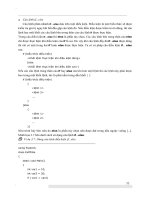
• Look at a rectangle whose length is n +1 and width is n, we divide this rectangle into
several rectangles (see Figure 1). Thus its area must equals to
n(n + 1) =
n

i=1
i +
n

i=1
i
= 2 (1 + 2 + 3 + + n)
Hence,
1 + 2 + 3 + + n =
1
2
n(n + 1)
Figure 1
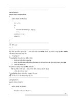
• Consider a rectangle whose length is
n

i=1
i and width is n + 1, we also divide this
rectangle into several rectangles (see Figure 2). Apply the above formula (i.e.
n

i=1
i =

1
2
n (n + 1) =
1
2
n
2
+
1
2
n), its area must equals to
14
2 THE SENSITIVITY

n

i=1
i

(n + 1) =
n

i=1
i
2
+
n

i=1
i


k=1
k

1
2
n
2
+
1
2
n

(n + 1) =
n

i=1
i
2
+
n

i=1

1
2
i
2
+
1

2
i

1
2
n
3
+ n
2
+
1
2
n =
n

i=1
i
2
+
1
2
n

i=1
i
2
+
1
2


1
2
n
2
+
1
2
n

1
2
n
3
+
3
4
n
2
+
1
4
n =
3
2
n

i=1
i
2
Hence,

1
2
+ 2
2
+ 3
2
+ + n
2
=
1
3
n
3
+
1
2
n
2
+
1
6
n
Figure 2
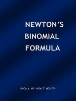
• Using this similar method, we can find out the sum of the cubes or the fourth powers
or more if we want. Thus we continue to view a rectangle whose length is
n

i=1
i
2

and
width is n + 1, we also divide this rectangle into several rectangles (see Figure 3).
Apply the above formulas (i.e.
n

i=1
i =
1
2
n (n + 1) =
1
2
n
2
+
1
2
n and
n

i=1
i
2
=
1
3
n
3
+
1

2
n
2
+
1
6
n), its area must equals to
15
2 THE SENSITIVITY

n

i=1
i
2

(n + 1) =
n

i=1
i
3
+
n

i=1
i

k=1
k

2

1
3
n
3
+
1
2
n
2
+
1
6
n

(n + 1) =
n

i=1
i
3
+
n

i=1

1
3
i

3
+
1
2
i
2
+
1
6
i

1
3
n
4
+
5
6
n
3
+
2
3
n
2
+
1
6
n =
n


i=1
i
3
+
1
3
n

i=1
i
3
+
1
2

1
3
n
3
+
1
2
n
2
+
1
6
n


+
1
6

1
2
n
2
+
1
2
n

1
3
n
4
+
2
3
n
3
+
1
3
n
2
=
4
3

n

i=1
i
3
Hence,
1
3
+ 2
3
+ 3
3
+ + n
3
=
1
4
n
4
+
1
2
n
3
+
1
4
n
2
Figure 3

At that time, the definition of fractional exponents is not correct, people still have a
question for its existence. For example, the concept of this is suggested in various ways in
the works of Oresme (14
th
century), Girard and Stevin (16
th
century).
The Geometry, first published in 1638, of René Descartes was the first published treatise
to use positive integer exponents written as superscripts. He saw exponents as an index for
repeated multiplication. That is to say he wrote x
3
in place of xxx. Wallis adopted this use
of an index and tried to extend it, and tested its validity across multiple representations.
Wallis took from Fermat the idea of using an equation to generate a curve, which was in
contrast to Descartes’ work which always began with a geometrical construction. Descartes
always constructed a curve geometrically first, and then analyzed it by finding its equa-
tion. Wallis mixed these ideas, so he defined what is the fractional exponents and proved
its existence successful.
And the Arithmetica Infinitorum contains a detailed investigation of the behavior
of sequences and ratios of sequences from which a variety of geometric results are then
concluded. We shall look at one of the most important examples. Consider the ratio of the
sum of a sequence of a fixed power to a series of constant terms all equal to the highest
value appearing in the sum. Wallis researched into ratios of the form :
A =
0
k
+ 1
k
+ 2
k

+ + n
k
n
k
+ n
k
+ n
k
+ + n
k
16
2 THE SENSITIVITY
For each fixed integer value of k, Wallis investigated the behavior of these ratios as n
increases. When k = 1, he calculates :
0 + 1 + 2
2 + 2 + 2
=
1
2
0 + 1 + 2 + 3
3 + 3 + 3 + 3
=
1
2
0 + 1 + 2 + 3 + 4
4 + 4 + 4 + 4 + 4
=
1
2
=

This can be seen from the well known Alhazen’s fomulas. We have
A =
n

i=1
i
n (n + 1)
=
n (n + 1)
2
n (n + 1)
=
1
2
Then Wallis called
1
2
the characteristic ratio of the index k = 1.
When k = 2, Wallis continued to compute the following ratios :
0
2
+ 1
2
1
2
+ 1
2
=
1
3

+
1
6
0
2
+ 1
2
+ 2
2
2
2
+ 2
2
+ 2
2
=
1
3
+
1
12
0
2
+ 1
2
+ 2
2
+ 3
2
3

2
+ 3
2
+ 3
2
+ 3
2
=
1
3
+
1
18
0
2
+ 1
2
+ 2
2
+ 3
2
+ 4
2
4
2
+ 4
2
+ 4
2
+ 4

2
+ 4
2
=
1
3
+
1
24
0
2
+ 1
2
+ 2
2
+ 3
2
+ 4
2
+ 5
2
5
2
+ 5
2
+ 5
2
+ 5
2
+ 5

2
+ 5
2
=
1
3
+
1
30
=
Wallis claimed that the right hand side is always equals
1
3
+
1
6n
and this can be checked
by Alhazen’s fomulas.
A =
n

i=1
i
2
n
2
(n + 1)
=
1
6

n (n + 1) (2n + 1)
n
2
(n + 1)
=
1
3
+
1
6n
As n increases this ratio approaches
1
3
(we can see lim
n→∞

1
3
+
1
6n

=
1
3
now), so Wallis
then defined the characteristic ratio of the index k = 2 as equal to
1
3
. In a similar way,

Wallos computed the characteristic ratio of k = 3 as
1
4
, and k = 4 as
1
5
and so forth.
Thus he made the general claim that the characteristic ratio of the index k is
1
k + 1
for all
positive integers.
17
2 THE SENSITIVITY
Next, Wallis show that these characteristic ratios yielded most of the familiar ratios
of area and volume known from geometry. It means he showed that his arithmetic was
consistent with the accepted truths of geometry.
He assumed that an area is a sum of an infinite number of parallel line segments, and
that a volume is a sum of an infinite number of parallel areas, his basis assumptions were
taken from Cavalieri’s Geometria Indivisibilibus Continuorum which was published
in 1635. Wallis first considered the area under the curve y = x
k
(see Figure 4). He wanted
to compute the ratio of the shaded area to the area of the rectangle which encloses it.
Figure 4
Wallis claimed that this geometric problem is an example of the characteristic ratio of
the sequence with index k. In specific, the terms in the numerator are the lengths of the
line segments that make up the shaded area while the terms in the denominator are the
lengths of the line segments that make up the rectangle (hence constant). He imagined
the increment or scale as very small while the number of the terms is very large.

And then this characteristic ratio of
1
3
holds for all parabolas, not just y = x
2
. In detail,
we can use Riemann’s integral for proving that results.
Consider a set [0; 1] and a curve y = 5x
2
, we have an area under this curve (S
1
) which is
calculated :
S
1
=
ˆ
1
0
5x
2
dx = 5

x
3
3

1
0
=

5
3
An area of a rectangle which encloses this curve (S
2
) equals 5, so that we have
S
1
=
1
3
S
2
This example means that characteristic ratio depends only on the exponent and not on
the coefficient, or we can say that characteristic ratio is not linear.
18
2 THE SENSITIVITY
Figure 5
In addition, that above ratio also shows that the volume of a pyramid is
1
3
of the box that
surrounds it (see Figure 5). Hence Wallis saw this as another example of his computation
of the characteristic ratio for the index k = 2.
These geometric results were not knew. Fermat, Roberval, Cavalieri and Pascal had all
previously made this claim that when k is a positive integer; the area under the curve
y = x
k
had a ratio of
1
k + 1

to the rectangle that encloses it. However, Wallis went on to
assert that if we define the index of
√
x as
1
2
, the claim remains true. Since the area under
the curve y =
√
x is the complement of the area under y = x
2
(i.e. the unshaded area
in Figure 4), it must have a characteristic ratio of
2
3
=
1
1
2
+ 1
. The same can be seen for
y =
3
√
x, whose characteristic ratio must be
3
4
=
1
1

3
+ 1

It was this coordination of two separate representations that gave Wallis the confidence
to claim that the appropriate index of y =
q
√
x
p
must be
p
q
, and that its characteristic ratio
must be
1
p
q
+ 1
. Wallis continued to assert that this claim remained true even when the
index is irrational because he gave
√
3 as an example. But in many cases, Wallis had no
way to directly verify the characteristic ratio of an index, for example : y =
3
√
x
2
.
How can we determine the characteristic ratio of the circle? This is the question that
motivated Wallis to study a particular family of curves from which he could interpolate

the value for circle. He wrote the equation of the circle of radius r, as y =
√
r
2
− x
2
, and
considered it in the first quadrant. He wanted to determine the ratio of its area to the r by
square that contains it.
Of course Wallis knew that this ratio is
π
4
, from various geometric constructions going
back to Archimedes, but he wanted to test his theory of index, characteristic ratio and
interpolation by arriving at this result in a new way. Therefore, he considered the family
of curves defined by the equations y = (
q
√
r −
q
√
x)
p
. Its graphs is showed in the unit square
(r = 1) (see Figure 6).
19
2 THE SENSITIVITY
Figure 6
If p and q are both integers, he knew that by expanding the binomial (
q

√
r −
q
√
x)
p
to the
p
th
power and using his rule for characteristic ratios he could determine the ratio for these
curves. For example, when p = q = 2, then : y = (
√
r −
√
x)
2
= r −2
√
r
√
x + x, and so must
have a characteristic ratio of 1 −2.
2
3
+
1
2
=
1
6

.
Figure 7
Next, Wallis, Pascal and others made a table of these ratios after computing it when p
and q are integers. This table records the ratio of the rectangle to the shaded area for each
of the curves y = (
q
√
r −
q
√
x)
p
. (see Table 1)
20
2 THE SENSITIVITY
Table 1
At this point, Wallis temporarily abandoned both the geometric and algebraic represen-
tations and began to work solely in the table representation. The question then became,
how does one interpolate the missing values in this table? Firstly, he worked on the rows
with integer values of q. We can summarize his works :
• When q = 0, we see the constant value of 1.
• When q = 1, we see an arithmetic progression whose common difference is
1
2
.
• In the row q = 2, we have the triangular numbers which are the sums of the integers
in the row q = 1. Thus we can use the formula for the sum of consecutive integers,
s
2
+ s

2
, where s = p + 1. Putting the intermediate values into this formula allows us
to complete the row q = 2. For example, letting s =
3
2
in this formula yields
15
8
, which
becomes the entry where p =
1
2
.
• The numbers in the row q = 3 are the pyramidal numbers each of which is the sum
of integers in the row q = 2. Hence the appropriate formula is found by summing the
formula from the row q = 2. Applying Alhazen’s formulas and then collecting terms,
we gain
1
2
s

i=1
i
2
+ i =
s
3
+ 3s
2
+ 2s

6
, where s = p + 1. For example, letting s =
3
2
, the
formula yields
105
48
, which becomes the table entry where p =
1
2
.
• In a similar fashion, we sum the previous cubic formula to obtain a formula for
the row q = 4. Using the Alhazen’s formulas and then collecting terms, we get
s
4
+ 6s
3
+ 11s
2
+ 6s
24
, where s = p + 1.
Therefore, Wallis built the following table by Ahazen’s formulas and his formulas for in-
terpolation. Since the table is symmetrical this also allows us to fill in the corresponding
columns when p is an integer. (see Table 2)
21
2 THE SENSITIVITY
Table 2
Wallis began to turn his attention to the row q =

1
2
. Each of the entries that now appear
there is calculated by using each of the successive interpolation formulas. And he see that
each of these formulas has a higher algebraic degree.
What pattern exists in the formation of these numbers which will allow us to interpolate
between them to find the missing entries? Remember that the first missing entry is the
q = p =
1
2
(i.e. the ratio of the square to the area of the quarter circle), we can find the
characteristic ratio of this as equals to
4
π
.
Hence Wallis first tried to fill in this row with arithmetic averages. The average of 1 and
3
2
is
5
4
, so this is not equal to
4
π
.
Wallis now observed that each of the numerators in these fractions is the product of
consecutive odd integers, while each of the denominators is the product of consecutive even
intergers; this means
15
8

=
3.5
2.4
;
105
48
=
3.5.7
2.4.6
;
945
384
=
3.5.7.9
2.4.6.8
. Hence to move two entries to
the right in this row one multiplies by
n
n −1
.
For the entries that appear so far, n is always odd; so Wallis assumed that to get from
one missing entry to the next one, he should still multiply by
n
n −1
, but this time n would
have to be the intermediate even number. Denoting the first missing entry by Ω whose
coefficient is 1, then the next missing entry should be 1.
4
4 −1
=

4
3
, so its result is
4
3
Ω. In a
similar fashion, we get the one after should be
4.6
3.5
Ω =
8
5
Ω, and the one after that should
be
4.6.8
3.5.7
Ω =
64
35
Ω and so forth.
22
2 THE SENSITIVITY
Then the q =
1
2
row becomes :
So the column p =
1
2
can now be filled in by symmetry. The row q =

3
2
has a similar
pattern (i.e. products of consecutive odd over consecutive enven number) but there the
entries two spaces to the right are always multiply by
n
n −3
(note that we go on n = 6).
We can also double check, as Wallis did, that this law of formation agrees with usual law
for the formation of binomials (i.e. each entry is the sum the entries two up, and two to
the left). The full table now show on Table 3 :
Table 3
Wallis saw that he could evaluate π which is put in Ω. He had to find a way to calculate
Ω using his priciple of interpolation so that he could check his value against the one known
from geometry.
Thus returning once again to the row q =
1
2
where moving two spaces to the right from
the n
th
entry multiplies that entry by
n
n −1
, Wallis noted that as n increases the fraction
n
n −1
gets closer and closer to 1

i.e. lim

n→∞
n
n −1
= 1

. Hence the number two spaces to
the right must change very little as we go further out the sequence. This is true of the
calculated fractions as well as the multiples of Ω.
23
2 THE SENSITIVITY
Wallis argued that since the whole sequence is increasing steadily, that consecutive
terms must also be getting close to 1 as we proceed. Hence he built these terms to be-
come
4.6.8.10
3.5.7.9
Ω ≈
3.5.7.9
2.4.6.8
Ω ≈
3.3.5.5.7.7.9.9
2.4.4.6.6.8.8.10
Because of
4
π
= Ω, hence
π = 2.
2.2.4.4.6.6.8.8
1.3.3.5.5.7.7.9
The empirical methods of Wallis led the young Isaac Newton to his first profound math-
ematical creation; the expansion of functions in binomial series. Thus Wallis’ method of

interpolation became for Newton the basis of his notion of continuity. So Newton wanted
to generalize the methods of Wallis
24