Intelligent Control and Computer Engineering
Bạn đang xem bản rút gọn của tài liệu. Xem và tải ngay bản đầy đủ của tài liệu tại đây (9.96 MB, 328 trang )
Lecture Notes in Electrical Engineering
Vo l u m e 7 0
For other titles published in this series, go to
www.springer.com/series/7818
Sio-Iong Ao
Oscar Castillo
Xu Huang
Editors
Intelligent
Control
and Computer
Engineering
Editors
Sio-Iong Ao
International Association of Engineers
Hung To Road 37-39
Hong Kong, Unit 1, 1/F
People’s Republic of China
Oscar Castillo
Tijuana Institute of Technology
Computer Science
Tijuana
Mexico
Xu Huang
University of Canberra
Fac. Information Science & Engineering
Canberra, Aust. Capital Terr.
Australia
ISSN 1876-1100
ISBN 978-94-007-0285-1
e-ISSN 1876-1119
e-ISBN 978-94-007-0286-8
DOI 10.1007/978-94-007-0286-8
Springer Dordrecht Heidelberg London New York
© Springer Science+Business Media B.V. 2011
No part of this work may be reproduced, stored in a retrieval system, or transmitted in any form or by
any means, electronic, mechanical, photocopying, microfilming, recording or otherwise, without written
permission from the Publisher, with the exception of any material supplied specifically for the purpose
of being entered and executed on a computer system, for exclusive use by the purchaser of the work.
Cover design: VTEX, Vilnius
Printed on acid-free paper
Springer is part of Springer Science+Business Media (www.springer.com)
A large international conference on Advances in Intelligent Control and Computer
Engineering was held in Hong Kong, March 17–19, 2010, under the auspices of
the International MultiConference of Engineers and Computer Scientists (IMECS
2010). The IMECS is organized by the International Association of Engineers
(IAENG). IAENG is a non-profit international association for the engineers and
the computer scientists, which was founded in 1968 and has been undergoing rapid
expansions in recent years. The IMECS conferences have served as excellent venues
for the engineering community to meet with each other and to exchange ideas.
Moreover, IMECS continues to strike a balance between theoretical and application
development. The conference committees have been formed with over two hundred
and fifty members who are mainly research center heads, deans, department heads
(chairs), professors, and research scientists from over thirty countries. The confer-
ence participants are also truly international with a high level of representation from
many countries. The responses for the conference have been excellent. In 2010,
we received more than one thousand manuscripts, and after a thorough peer review
process 56.26% of the papers were accepted ( />This volume contains 25 revised and extended research articles written by promi-
nent researchers participating in the conference. Topics covered include artificial
intelligence, control engineering, decision supporting systems, automated planning,
automation systems, systems identification, modelling and simulation, communica-
tion systems, signal processing, and industrial applications. The book offers the state
of the art of tremendous advances in intelligent control and computer engineering
and also serves as an excellent reference text for researchers and graduate students,
working on intelligent control and computer engineering.
Sio-Iong Ao
Oscar Castillo
Xu Huang
v
Intelligent Control of Reduced-Order Closed Quantum Computation
Systems Using Neural Estimation and LMI Transformation 1
Anas N. Al-Rabadi
Optimal Guidance and Control for Space Robot Operation 15
Takuro Kobayashi and Shinichi Tsuda
The Application of Genetic Algorithms in Designing Fuzzy Logic
Controllers for Plastic Extruders 25
Ismail Yusuf, Nur Iksan, and Nanna Suryana Herman
Automatic Weight Selection and Fixed-Structure Cascade Controller for
a Quadratic Boost Converter 39
Somyot Kaitwanidvilai and Pitsanu Srithongchai
Availability Studies and Solutions for Wheeled Mobile Robots 47
Adrian Korodi and Toma L. Dragomir
The Use of Higher-Order Spectrum for Fault Quantification of
Industrial Electric Motors 59
Juggrapong Treetrong
A Newly Cooperative PSO – Multiple Particle Swarm Optimizers with
Diversive Curiosity, MPSOα/DC 69
Hong Zhang
Predicting the Toxicity of Chemical Compounds Using GPTIPS: A Free
Genetic Programming Toolbox for MATLAB 83
Dominic P. Searson, David E. Leahy, and Mark J. Willis
Diversity-Driven Self-adaptation in Evolutionary Algorithms 95
Fanchao Zeng, James Decraene, Malcolm Yoke Hean Low, Suiping
Zhou, and Wentong Cai
vii
viii Contents
A New Rearrangement Plan for Freight Cars in a Train 107
Yoichi Hirashima
Coevolving Negotiation Strategies for P-S-Optimizing Agents 119
Jeonghwan Gwak and Kwang Mong Sim
Policy Gradient Approach for Learning of Soccer Player Agents 137
Harukazu Igarashi, Hitoshi Fukuoka, and Seiji Ishihara
Genetic Algorithm for Forming Buyer Coalition with Bundles of Items
in E-Marketplaces 149
Anon Sukstrienwong
Inside Virtual CIM 163
Ning Zhou, Sev Naglingam, Ke Xing, and Grier Lin
Supreme Court Sentences Retrieval Using Thai Law Ontology 177
Tanapon Tantisripreecha and Nuanwan Soonthornphisaj
Genetic Algorithm Based Model for Effective Document Retrieval 191
Hazra Imran and Aditi Sharan
An Agent-Based Cloud Service Discovery System that Consults a Cloud
Ontology 203
Taekgyeong Han and Kwang Mong Sim
Possible Applications of Navigation Tools in Tilings of Hyperbolic Spaces 217
Maurice Margenstern
Graph Pattern Matching with Expressive Outerplanar Graph Patterns . 231
Hitoshi Yamasaki, Takashi Yamada, and Takayoshi Shoudai
Setvectors – An Efficient Method to Predict Cache Contention 245
Michael Zwick
New Material Model for Describing Large Deformation of Pressure
Sensitive Adhesive 259
Kazuhisa Maeda, Shigenobu Okazawa, and Koji Nishiguchi
QoS Provisioning in EPON Systems with Interleaved Two Phase
Polling-Based DBA 271
I-Shyan Hwang, Jhong-Yue Lee, and Zen-Der Shyu
The Game of n-Player Shove and Its Complexity 285
Alessandro Cincotti
Contents ix
Modeling the Vestibular Nucleus 293
Alexandru Codrean, Adrian Korodi, Toma-Leonida Dragomir, and Vlad
Ceregan
SPECT Lung Delineation 307
Alex Wang and Hong Yan
Quantum Computation Systems Using Neural
Estimation and LMI Transformation
Anas N. Al-Rabadi
Abstract A new method of intelligent control for closed quantum computation
time-independent systems is introduced. The introduced method uses recurrent su-
pervised neural computing to identify certain parameters of the transformed system
matrix [
˜
A]. Linear matrix inequality (LMI) is then used to determine the permuta-
tion matrix [P]so that a complete system transformation {[
˜
B], [
˜
C], [
˜
D]}is achieved.
The transformed model is then reduced using singular perturbation and state feed-
back control is implemented to enhance system performance. In quantum computa-
tion and mechanics, a closed system is an isolated system that can’t exchange energy
or matter with its environment and doesn’t interact with other quantum systems. In
contrast to an open quantum system, a closed quantum system obeys the unitary
evolution and thus is information lossless that implies state reversibility. The exper-
imental simulations show that the new hierarchical control simplifies the model of
the quantum computing system and thus uses a simpler controller that produces the
desired performance enhancement and system response.
Keywords Linear matrix inequality · Model reduction · Quantum computation ·
Recurrent supervised neural computing · State feedback control system
1 Introduction
Due to the fact that current dense hardware implementations are heading towards
the critical atomic threshold, quantum computing will rapidly occupy an increas-
ingly important position in building nano-size, super-fast, and ultra-low power con-
suming systems [1–3, 6, 8, 12]. Other motivations for implementing circuits and
systems using quantum computing would include items such as: (1) power where
A.N. Al-Rabadi (
)
The University of Jordan, Faculty of Engineering & Technology, Computer Engineering
Department, Amman, Jordan 11942
e-mail:
S I. Ao et al. (eds.), Intelligent Control and Computer Engineering,
Lecture Notes in Electrical Engineering 70,
DOI 10.1007/978-94-007-0286-8_1, © Springer Science+Business Media B.V. 2011
1
2 A.N. Al-Rabadi
State Feedback Control System
Model Reduction
System Transformation: {[
˜
B], [
˜
C], [
˜
D]}
LMI-Based Permutation Matrix: [P]
Neural-Based State Transformation: [
˜
A]
Time-Independent Quantum Computing System: {[A], [B], [C], [D]}
Fig. 1 The introduced control methodology utilized for closed quantum computing systems
the internal computations in quantum computing systems consume no power and
only power is consumed when reading and writing operations are performed [1, 6,
8, 12]; (2) size where, at the atomic dimension, quantum mechanical effects have to
be accounted for; and (3) speed where if the properties of superposition and entan-
glement of quantum mechanics can be usefully employed in the design of circuits
and systems, significant computational speed enhancements can be expected [1, 6,
12]. Figure 1 illustrates the layer layout of the introduced closed-system quantum
computing control methodology.
2 Fundamentals
This section presents important background on quantum computing systems, super-
vised neural networks, linear matrix inequality, and model order reduction that will
be used later in Sects. 3, 4 and 5.
2.1 Quantum Computation
Quantum computing is an efficient method of computation that uses the dynamic
process which is governed by the Schrödinger equation [1, 6, 12]. The one-
dimensional time-dependent Schrödinger equation (TDSE) is as follows [1, 5, 6,
12]:
−
(h/2π)
2
2m
∂
2
|ψ
∂x
2
+V |ψ=i(h/2π)
∂|ψ
∂t
(1)
or H |ψ=i(h/2π)
∂|ψ
∂t
(2)
where h is Planck constant (6.626 ·10
−34
J ·s =4.136 ·10
−15
eV ·s), V(x,t)is the
applied potential, m is the particle mass, i is the imaginary number, |ψ(x,t) is the
quantum state, H is the Hamiltonian operator where H =−[(h/2π)
2
/2m]∇
2
+V ,
and ∇
2
is the Laplacian operator.
Intelligent Control of Reduced-Order Closed Quantum Computation Systems 3
A general solution to the TDSE is the expansion of a stationary (i.e., time-
independent for spatial) basis functions (i.e., eigen states) U
e
(r) using time-
dependent (i.e., temporal) expansion coefficients c
e
(t) as follows:
(r,t) =
n
e=0
c
e
(t)u
e
(r)
The expansion coefficients c
e
(t) are a scaled complex exponentials as follows:
c
e
(t) =k
e
e
−i
E
e
(h/2π)
t
where E
e
are the energy levels. In quantum computing, the time-independent
Schrödinger equation (TISE) is normally used [1, 12]:
∇
2
ψ =
2m
(h/2π)
2
(V −E)ψ (3)
where the solution |ψ is an expansion over orthogonal basis states |φ
i
defined in
a linear complex vector space called Hilbert space H as:
|ψ=
i
c
i
|φ
i
(4)
where the coefficients c
i
are called probability amplitudes and |c
i
|
2
is the probability
that the quantum state |ψ will collapse into the (eigen) state |φ
i
. The probability
is equal to the inner product |φ
i
|ψ|
2
, with the unitary condition
|c
i
|
2
= 1. In
quantum computing, a linear and unitary operator is used to transform an input
vector of qu
antum bits (qubits) into an output vector of qubits. In the two-valued
quantum computing, the qubit is a vector of bits which is defined as follows [1, 12]:
qubit
0
≡|0=
1
0
, qubit
1
≡|1=
0
1
(5)
A two-valued quantum state |ψ is a superposition of quantum basis states |φ
i
.
Thus, for the orthonormal computational basis states {|0, |1}, one has the following
quantum state:
|ψ=α|0+β|1 (6)
where αα
∗
=|α|
2
= p
0
≡ the probability of having state |ψ in state |0,ββ
∗
=
|β|
2
=p
1
≡ the probability of having state |ψ in state |1, and |α|
2
+|β|
2
=1. The
calculation in quantum computing for multiple systems follows the tensor product
(⊗). For example, given the quantum states |ψ
1
and |ψ
2
, one has:
|ψ
1
ψ
2
=|ψ
1
⊗|ψ
2
=
α
1
|0+β
1
|1
⊗
α
2
|0+β
2
|1
= α
1
α
2
|00+α
1
β
2
|01+β
1
α
2
|10+β
1
β
2
|11 (7)
A physical system (e.g., the hydrogen atom) that is described by the following
equation:
|ψ=c
1
|Spinup+c
2
|Spindown (8)
4 A.N. Al-Rabadi
can be used to physically implement a two-valued quantum computing. Another
common alternative form of Eq. 8 is as follows:
|ψ=c
1
+
1
2
+c
2
−
1
2
(9)
Many-valued quantum computing can also be performed. For the three-valued
case, the qubit becomes a 3D vector qu
antum discrete digit (qudit), and in general,
for an m-valued quantum computing the qudit is of dimension “many” [1, 12]. For
example, one has for the 3-state case, the following qudits:
qudit
0
≡|0=
1
0
0
, qudit
1
≡|1=
0
1
0
, qudit
2
≡|2=
0
0
1
(10)
A three-valued quantum state is a superposition of three quantum orthonormal basis
states (vectors). Thus, for the orthonormal computational basis states {|0, |1, |2},
one has the following quantum state:
|ψ=α|0+β|1+γ |2
where αα
∗
=|α|
2
= p
0
≡ the probability of having state |ψ in state |0,ββ
∗
=
|β|
2
=p
1
≡ the probability of having state |ψ in state |1,γγ
∗
=|γ |
2
=p
2
≡ the
probability of having state |ψ in state |2, and |α|
2
+|β|
2
+|γ |
2
=1.
The calculation in quantum computing for m-valued multiple systems follow
the tensor product in a manner similar to the one demonstrated for the higher-
dimensional qubit in the two-valued quantum computing. Several quantum comput-
ing systems were used to implement quantum gates from which complete quantum
circuits and systems were constructed [1, 6, 12], where several of the two-valued
and m-valued quantum circuit implementations use the two-valued and m-valued
quantum Swap-based and Not-based gates [1, 12].
In general, for an m-valued logic, a quantum state is a superposition of m quan-
tum orthonormal basis states (i.e., vectors). Thus, for the orthonormal computational
basis states {|0, |1, ,|m −1}, one has the quantum state:
|ψ=
m−1
k=0
c
k
|q
k
(11)
where
m−1
k=0
c
k
c
∗
k
=
m−1
k=0
|c
k
|
2
= 1. The calculation in quantum computing for
m-valued multiple systems is done similar to the case for the two-valued system.
In quantum mechanical systems, a closed system is an isolated system that
doesn’t exchange energy or matter with its environment (i.e., doesn’t dissipate
power) and doesn’t interact with other quantum systems. While an open quantum
system interacts with its environment and thus dissipates power which results in a
non-unitary evolution producing information loss, a closed quantum system doesn’t
exchange energy or matter with its environment and therefore doesn’t dissipate
power which results in a unitary evolution (i.e., unitary matrix) and thus it is in-
formation lossless.
Intelligent Control of Reduced-Order Closed Quantum Computation Systems 5
Fig. 2 The utilized second
order recurrent neural
network architecture, where
the estimated matrices are
given by
{
˜
A
d
=
A
11
A
12
A
21
A
22
,
˜
B
d
=
B
11
B
21
}
and W =[
[
˜
A
d
][
˜
B
d
]
w]
2.2 Recurrent Supervised Neural Computations
The supervised recurrent neural network which is used for the estimation in this
research is based on an approximation of the method of steepest descent [2, 9]. The
network tries to match the output of certain neurons to the desired values of the
system output at a specific instant of time. Figure 2 shows a network consisting of
a total of N neurons with M external input connections for a 2
nd
order system with
two neurons and one external input, where the variable g(k) denotes the (M × 1)
external input vector which is applied to the network at discrete time k and the
variable y(k +1) denotes the corresponding (N × 1) vector of individual neuron
outputs produced one step later at time (k +1).
The derivation of the recurrent algorithm can be started by using d
j
(k) to denote
the desired (i.e., target) response of neuron j at time k, and ς(k) to denote the set
of neurons that are chosen to provide externally reachable outputs. A time-varying
(N × 1) error vector e(k) is defined whose j
th
element is given by the following
relationship:
e
j
(k) =
d
j
(k) −y
j
(k), if j ∈ς(k)
0, otherwise
The objective is to minimize the cost function E
total
which is obtained by E
total
=
k
E(k) where E(k) =
1
2
j∈ς
e
2
j
(k). The dynamical system is described by the
following triply indexed set of variables (π
j
m
):
π
j
m
(k) =
∂y
j
(k)
∂w
m
(k)
where for every time step k and all appropriate j, m and , system dynamics are
controlled by:
π
j
m
(k +1) =˙ϕ
v
j
(k)
i∈β
w
ji
(k)π
i
m
(k) +δ
mj
u
(k)
6 A.N. Al-Rabadi
with π
j
m
(0) = 0. The values of π
j
m
(k) and the error signal e
j
(k) areusedtocom-
pute the corresponding weight changes with a learning rate (η):
w
m
(k) =η
j∈ς
e
j
(k)π
j
m
(k) (12)
Using the weight changes, the updated weight w
m
(k +1) is calculated as:
w
m
(k +1) =w
m
(k) +w
m
(k) (13)
and repeating this computation procedure provides the minimization of the cost
function and the objective is therefore achieved.
2.3 Transformation via Linear Matrix Inequality
In this sub-section, the detailed illustration of system transformation using LMI
optimization will be presented [2]. Consider the system:
˙x(t) =Ax(t) +Bu(t) (14)
y(t) =Cx(t) +Du(t) (15)
In order to determine the transformed [A] matrix, which is [
˜
A], the discrete zero
input response is obtained. This is achieved by providing the system with some
initial state values and setting the system input to zero (i.e., u(k) =0). Hence, the
discrete system of Eqs. 14, 15, with the initial condition x(0) =x
0
, becomes:
x(k +1) =A
d
x(k) (16)
y(k) =x(k) (17)
We need x(k) as a neural network target to train the network to obtain the needed
parameters in [
˜
A
d
] such that the system output will be the same for [A
d
] and [
˜
A
d
].
Hence, simulating this system provides the state response corresponding to their
initial values with only the [A
d
] matrix is being used. Once the input-output data is
obtained, transforming the [A
d
] matrix is achieved using the neural network train-
ing, as will be explained in Sect. 3. The estimated transformed [A
d
] matrix is then
converted back into the continuous form which yields:
˜
A =
A
r
A
c
0 A
o
(18)
Having the [A]and [
˜
A] matrices, the permutation [P]matrix is determined using
the LMI optimization technique [2, 4] as will be illustrated in later sections. The
complete system transformation can be achieved by assuming that ˜x = P
−1
x and
then the system of Eqs. 14, 15 can be re-written as follows:
P
˙
˜x(t) =AP ˜x(t) +Bu(t), ˜y(t) =CP ˜x(t) +Du(t)
Intelligent Control of Reduced-Order Closed Quantum Computation Systems 7
where ( ˜y(t) =y(t)). Pre-multiplying the first equation above by [P
−1
], one obtains
{P
−1
P
˙
˜x(t) =P
−1
AP ˜x(t)+P
−1
Bu(t), ˜y(t) =CP ˜x(t)+Du(t)} which yields the
following transformed model:
˙
˜x(t) =
˜
A ˜x(t) +
˜
Bu(t) (19)
˜y(t) =
˜
C ˜x(t) +
˜
Du(t) (20)
where the transformed system matrices are given by:
˜
A =P
−1
AP (21)
˜
B =P
−1
B (22)
˜
C =CP (23)
˜
D =D (24)
Transforming the system matrix [A] into the form shown in Eq. 18 can be achieved
based on the property of matrix reducability [2, 10].
2.4 Singular Perturbation for Model Order Reduction
Linear time-invariant models of many systems have fast and slow dynamics which
is referred to as singularly perturbed systems [2, 11]. Neglecting the fast dynamics
of a singularly perturbed system provides a reduced slow model leading to simpler
controllers based on the reduced model information [2, 11]. For reduced system
formulation, consider the following singularly perturbed system:
˙x(t) =A
11
x(t) +A
12
ξ(t)+B
1
u(t), x(0) =x
0
(25)
ε
˙
ξ(t)=A
21
x(t) +A
22
ξ(t)+B
2
u(t), ξ(0) =ξ
0
(26)
y(t) =C
1
x(t) +C
2
ξ(t) (27)
where x ∈
m
1
and ξ ∈
m
2
are the slow and fast state variables, respectively, u ∈
n
1
and y ∈
n
2
are the input and output vectors, respectively, {[A
ii
], [B
i
], [C
i
]}
are constant matrices of appropriate dimensions with i ∈{1, 2}, and ε is a small
positive constant. The singularly perturbed system in Eqs. 25, 26, 27 is simplified
for ε =0. By doing the above step, one neglects the system fast dynamics assuming
that the state variables ξ have reached the quasi-steady state. Setting ε =0inEq.26
and assuming [A
22
] is nonsingular, produces:
ξ(t)=−A
−1
22
A
21
x
r
(t) −A
−1
22
B
1
u(t) (28)
where the index r denotes remained (or reduced) model. By substituting Eq. 28 into
Eqs. 25, 26, 27, one obtains the following reduced order model:
˙x
r
(t) =A
r
x
r
(t) +B
r
u(t) (29)
y(t) =C
r
x
r
(t) +D
r
u(t) (30)
for {A
r
=A
11
−A
12
A
−1
22
A
21
,B
r
=B
1
−A
12
A
−1
22
B
2
,C
r
=C
1
−C
2
A
−1
22
A
21
,D
r
=
−C
2
A
−1
22
B
2
}.
8 A.N. Al-Rabadi
3 Neural Estimation with Linear Matrix Inequality-Based
Transformation for Closed Reduced-Order Quantum
Computation Systems
In this work, it is our objective to search for a similarity transformation that can be
utilized within the context of closed time-independent quantum computing systems
to decouple a pre-selected eigenvalue set from the system matrix [A]. To achieve this
objective, training the neural network to estimate the transformed discrete system
matrix [
˜
A
d
] is performed [2]. For the system of Eqs. 25, 26, 27, the discrete model
of the quantum computing system is obtained as:
x(k +1) =A
d
x(k)+B
d
u(k) (31)
y(k) =C
d
x(k)+D
d
u(k) (32)
The estimated discrete model of Eqs. 31, 32 can be re-written as:
˜x
1
(k +1)
˜x
2
(k +1)
=
A
11
A
12
A
21
A
22
˜x
1
(k)
˜x
2
(k)
+
B
11
B
21
u(k) (33)
˜y(k) =
˜x
1
(k)
˜x
2
(k)
(34)
where k is the time index, and the matrix elements of Eqs. 33, 34 were shown in
Fig. 2. The recurrent neural network that was presented in Sect. 2.2 can be sum-
marized by defining as the set of indices (i) for which g
i
(k)is an external input,
which is one external input in the quantum computing system, and by defining β
as the set of indices (i) for which y
i
(k) is an internal input (or a neuron output),
which is two internal inputs (i.e., two system states) in the quantum computing sys-
tem. Also, we define u
i
(k) as the combination of the internal and external inputs for
which i ∈β ∪. By using this setting, training the network depends on the internal
activity of each neuron which is given by the following equation:
v
j
(k) =
i∈∪β
w
ji
(k)u
i
(k) (35)
where w
ji
is the weight representing an element in the system matrix or input matrix
for j ∈β and i ∈β ∪ such that W =
[
˜
A
d
][
˜
B
d
]
. At the next time step (k +1),
the output (i.e., internal input) of the neuron j is computed by passing the activity
through the nonlinearity φ(.) as follows:
x
j
(k +1) =ϕ
v
j
(k)
(36)
With these equations, based on an approximation of the method of steepest descent,
the network estimates the system matrix [A
d
] as was shown in Eq. 16 for zero input
response. That is, an error can be obtained by matching a true state output with a
neuron output as follows:
e
j
(k) =x
j
(k) −˜x
j
(k)
Intelligent Control of Reduced-Order Closed Quantum Computation Systems 9
The objective is to minimize the cost function E
total
=
k
E(k) where E(k) =
1
2
j∈ς
e
2
j
(k) and ς denotes the set of indices j for the output of the neuron struc-
ture. This cost function is minimized by estimating the instantaneous gradient of
E(k) with respect to the weight matrix [W] and then updating [W] in the negative
direction of this gradient. In detailed steps, this may be proceeded as follows:
– Initialize the weights [W] by a set of uniformly distributed random numbers.
Starting at the instant k = 0, use Eqs. 35, 36 to compute the output values of the
N neurons (where N =β).
– For each time step k and all j ∈β, m ∈ β, and ∈β ∪, compute the dynamics
of the system governed by the triply indexed set of variables:
π
j
m
(k +1) =˙ϕ(v
j
(k))
i∈β
w
ji
(k)π
i
m
(k) +δ
mj
u
(k)
with initial conditions π
j
m
(0) =0 and δ
m
is given by (∂w
ji
(k)/∂w
m
(k)), which
is equal to “1” only when j = m and i = otherwise it is “0”. Note that for the
special case of a sigmoidal nonlinearity in the form of a logistic function, the
derivative ˙ϕ(·) is given by ˙ϕ(v
j
(k)) =y
j
(k +1)[1 −y
j
(k +1)].
– Compute the weight changes correspond to the error and system dynamics:
w
m
(k) =η
j∈ς
e
j
(k)π
j
m
(k) (37)
– Update the weights in accordance with:
w
m
(k +1) =w
m
(k) +w
m
(k) (38)
– Repeat the computation until the desired estimation is achieved.
As was illustrated in Eqs. 16, 17, for the purpose of estimating only the transformed
system matrix [
˜
A], the training is based on the zero input response. Once the train-
ing is complete, the obtained weight matrix [W] is the discrete estimated trans-
formed system matrix. Transforming the estimated system back to the continuous
form yields the desired continuous transformed system matrix [
˜
A].UsingtheLMI
optimization technique that was illustrated in Sect. 2.3, the permutation matrix [P]
is determined. Hence, a complete system transformation, as was shown in Eqs. 19,
20, is achieved. To perform the order reduction, the system in Eqs. 19, 20 are written
as:
˙
˜x
r
(t)
˙
˜x
o
(t)
=
A
r
A
c
0 A
o
˜x
r
(t)
˜x
o
(t)
+
B
r
B
o
u(t) (39)
˜y
r
(t)
˜y
o
(t)
=
[
C
r
C
o
]
˜x
r
(t)
˜x
o
(t)
+
D
r
D
o
u(t) (40)
where the system transformation enables us to decouple the original system into
retained (r) and omitted (o) eigenvalues. The retained eigenvalues are the dominant
eigenvalues that produce slow dynamics and the omitted eigenvalues are the non-
dominant eigenvalues that produce fast dynamics. Equation 39 can be re-written as
{
˙
˜x
r
(t) =A
r
˜x
r
(t) +A
c
˜x
o
(t) +B
r
u(t),
˙
˜x
o
(t) =A
o
˜x
o
(t) +B
o
u(t)}.
10 A.N. Al-Rabadi
The coupling term A
c
˜x
o
(t) maybe compensated for by solving for ˜x
o
(t) in the
second equation above by setting
˙
˜x
o
(t) to zero using the singular perturbation
method (by setting ε =0). Doing so, the following is obtained:
˜x
o
(t) =−A
−1
o
B
o
u(t) (41)
Using ˜x
o
(t), we get the reduced model given by:
˙
˜x
r
(t) =A
r
˜x
r
(t) +
−A
c
A
−1
o
B
o
+B
r
u(t) (42)
y(t) =C
r
˜x
r
(t) +
−C
o
A
−1
o
B
o
+D
u(t) (43)
Therefore, the overall reduced order model is:
˙
˜x
r
(t) =A
or
˜x
r
(t) +B
or
u(t) (44)
y(t) =C
or
˜x
r
(t) +D
or
u(t) (45)
where the details of the overall reduced matrices {[A
or
], [B
or
], [C
or
], [D
or
]} are
shown in Eqs. 42, 43.
4 Model Order Reduction of the Quantum Computation
Systems Using Neural Estimation and Linear Matrix
Inequality Transformation
Let us implement the time-independent quantum computing closed-system using the
particle in finite-walled box potential V for the general case of m-valued quantum
computing in which the resulting distinct energy states are used as the orthonormal
basis states [2]. The dynamical TISE of the one-dimensional particle in finite-walled
box potential V is expressed as follows:
∂
2
∂x
2
+
2m
(h/2π)
2
(E −V)=0
which also can be re-written as
∂
2
∂x
2
=
2m
2
(V −E), where m is the particle mass,
and = (h/2π) is the reduced Planck constant (which is also called the Dirac con-
stant)
∼
=
1.055 ·10
−34
J ·s =6.582 ·10
−16
eV ·s. Thus, for {x
1
=, x
2
=
∂
∂x
,x
1
=
x
2
,x
2
=
∂
2
∂x
2
}, the state space model of the time-independent closed quantum com-
puting system is given as:
x
1
x
2
=
01
2m(V −E)
2
0
x
1
x
2
+
0
0
u (46)
y = (
10
)
x
1
x
2
+(0)u (47)
For simulation reasons, Eqs. 46, 47 can also be re-written equivalently as:
Intelligent Control of Reduced-Order Closed Quantum Computation Systems 11
−x
2
x
1
=
0
2m(E−V)
2
−10
−x
2
x
1
+
0
0
u (48)
y =(
01
)
−x
2
x
1
+(0)u (49)
Also, for conducting the simulations, one may often need to scale the system
Eq. 48 without changing the system dynamics. Thus, by scaling both sides of Eq. 48
by a scaling factor a, the following set of equations is obtained:
a
−x
2
x
1
=a
0
2m(E−V)
2
−10
−x
2
x
1
+
0
0
u (50)
y =(
01
)
−x
2
x
1
+(0)u (51)
Therefore, one obtains the following set of quantum system matrices:
A =a
0
2m(E−V)
2
−10
(52)
B =
0
0
(53)
C =[
01
] (54)
D =[0] (55)
The specifications of the system matrix in Eq. 52 for the particle in finite-walled box
are determined by (1) potential box width L (in nanometer), (2) particle mass m,
and (3) the potential value V (i.e., potential height in electron Volt). As an example,
consider the particle in a finite-walled potential with specifications of (E − V)=
88 MeV and a very light particle with a particle mass of N =10
−33
of the electron
mass (where the electron mass m
e
∼
=
9.109 ·10
−27
g =5.684 ·10
−12
eV/(m/s)
2
).
This system was discretized using the sampling rate T
s
= 0.005 second and sim-
ulated for a zero input. Hence, based on the obtained simulated output data and
by using NN to estimate the subsystem matrix [A
c
] of Eq. 18 with a learning rate
η =0.015, the transformed system matrix [
˜
A]was obtained where [A
r
]is set to pro-
vide the dominant eigenvalues (i.e., slow dynamics) and [A
o
] is set to provide the
non-dominant eigenvalues (i.e., fast dynamics) of the original system. Thus, when
training the system, the second state ˜x
o
(t) of the transformed model in Eq. 39 is un-
changed due to the restriction of [
0 A
o
]seen in [
˜
A]. This may lead to an undesired
starting of the system response, but fast system overall convergence.
Using [
˜
A] along with [A], the LMI is implemented to obtain {[
˜
B], [
˜
C], [
˜
D]}
which makes a complete model transformation. Then, by using singular perturbation
for model reduction, the reduced order model is obtained. Thus, by implementing
the previously stated system specifications and by using the squared reduced Planck
constant of
2
= 43.324 ·10
−32
(eV ·s)
2
, one obtains the following scaled system
matrix from Eq. 52:
12 A.N. Al-Rabadi
Fig. 3 (Color online)
Input-to-output quantum
computing system step
responses: full-order system
model (solid blue line),
transformed reduced-order
model (dashed black line),
and non-transformed
reduced-order model (dashed
red line)
a
−1
A =
0
2m(E−V)
2
−10
∼
=
02.32 ·10
−6
−0.95 0.003
=
−1
5000
0 −0.0116
4761.9 −16
Accordingly, the eigenvalues were found to be {−5.0399, −10.9601}.Forastep
input, simulating the original and transformed reduced order models along with the
non-transformed reduced order model produced the results shown in Fig. 3.
5 The Design of State Feedback Controller for the
Reduced-Order Closed Quantum Models
In this research, since the closed quantum computing system is a 2
nd
order system
reduced to a 1
st
order, we will investigate the system stability and enhancing perfor-
mance by implementing the simple method of the s-domain pole replacement [2, 7].
For the reduced model in Eqs. 44, 45, a state feedback controller can be designed.
For example, this can be achieved by replacing the system eigenvalues with new
faster eigenvalues. Hence, let the control input be:
u(t) =−K ˜x
r
(t) +r(t) (56)
where K is to be designed based on the desired system eigenvalues.
Replacing the control input u(t) in Eqs. 44, 45 by the above new control input in
Eq. 56 yields the following reduced system:
˙
˜x
r
(t) =A
or
˜x
r
(t) +B
or
−K ˜x
r
(t) +r(t)
(57)
y(t) =C
or
˜x
r
(t) +D
or
−K ˜x
r
(t) +r(t)
(58)
which can be re-written as:
Intelligent Control of Reduced-Order Closed Quantum Computation Systems 13
Fig. 4 (Color online)
Enhanced system step
responses using pole
placement; full-order system
model (solid blue line),
transformed reduced model
(dashed black line),
non-transformed reduced
model (dashed red line), and
the controlled transformed
reduced (dashed pink line)
˙
˜x
r
(t) =A
or
˜x
r
(t) −B
or
K ˜x
r
(t) +B
or
r(t) →
˙
˜x
r
(t)
=[A
or
−B
or
K]˜x
r
(t) +B
or
r(t)
y(t) =C
or
˜x
r
(t) −D
or
K ˜x
r
(t) +D
or
r(t) →y(t)
=[C
or
−D
or
K]˜x
r
(t) +D
or
r(t)
The overall closed-loop model is then written as:
˙
˜x(t) =A
cl
˜x
r
(t) +B
cl
r(t) (59)
y(t) =C
cl
˜x
r
(t) +D
cl
r(t) (60)
such that the closed-loop system matrix [A
cl
] will provide the new desired eigen-
values. As an example, consider the following non-scaled quantum system:
A =
0 −0.385
142.857 −18
,B=
0.077
0
,C=[
01
],D=[0]
Using the transformation-based reduction technique, one obtains the reduced model
{
˙
˜x
r
(t) =[−3.901]˜x
r
(t) +[−5.255]u(t), y
r
(t) =[−0.197]˜x
r
(t) +[−0.066]u(t)}
with the eigenvalue of −3.901. Now, suppose that a new eigenvalue λ =−12 that
will produce faster system dynamics is desired for this reduced model. This objec-
tive is achieved by first setting the desired characteristic equation as λ +12 =0. To
determine the feedback control gain K, the characteristic equation is accordingly
utilized by using Eqs. 57–60 which yields {(λI −A
cl
) =0 →λI −[A
or
−B
or
K]=
0} after which the feedback control gain K is calculated to be −1.5413, and the
closed-loop system now has the eigenvalue of −12. Simulating the reduced model
using a sampling rate T
s
=0.005 second and a learning rate η =0.015 with the new
eigenvalue for the same original system input (i.e., step input) has generated the
response in Fig. 4.
14 A.N. Al-Rabadi
6 Conclusions and Future Work
A new method of intelligent control via neural estimation and LMI-based trans-
formation for controlling time-independent quantum computing systems is imple-
mented, and a simple state feedback control using pole placement was then applied
on the reduced quantum computing model that achieved the required system re-
sponse. Future work will investigate the implementation of the introduced hierar-
chical control onto other quantum systems such as the non-linear, relativistic, and
time-dependent quantum computing systems.
References
1. Al-Rabadi, A.N.: Reversible Logic Synthesis: From Fundamentals to Quantum Computing.
Springer, Berlin (2004)
2. Al-Rabadi, A.N.: Recurrent supervised neural computation and LMI model transformation for
order reduction-based control of linear time-independent closed quantum computing systems.
In: Lecture Notes in Engineering and Computer Science: Proc. of the Int. MultiConference
of Engineers and Computer Scientists, IMECS 2010, Hong Kong, 17–19 March 2010, pp.
911–923 (2010)
3. Bennett, C.H., Landauer, R.: The fundamental physical limits of computation. Sci. Am.
253(1), 48–56 (Jul 1985)
4. Boyd, S., El-Ghaoui, L., Feron, E., Balakrishnan, V.: Linear Matrix Inequalities in System and
Control Theory. SIAM, Philadelphia (1994)
5. Dirac, P.: The Principles of Quantum Mechanics. Oxford University Press, London (1930)
6. Feynman, R.: Quantum mechanical computers. Opt. News 11, 11–20 (1985)
7. Franklin, G., Powell, J., Emami-Naeini, A.: Feedback Control of Dynamic Systems. Addison-
Wesley, Reading (1994)
8. Fredkin, E., Toffoli, T.: Conservative logic. Int. J. Theor. Phys. 21, 219–253 (1982)
9. Haykin, S.: Neural Networks: A Comprehensive Foundation. Macmillan College, New York
(1994)
10. Horn, R., Johnson, C.: Matrix Analysis. Cambridge University Press, Cambridge (1985)
11. Kokotovic, P., O’Malley, R., Sannuti, P.: Singular perturbation and order reduction in control
theory – an overview. Automatica 12(2), 123–132 (1976)
12. Nielsen, M., Chuang, I.: Quantum Computation and Quantum Information. Cambridge Uni-
versity Press, Cambridge (2000)